Intelligent Fault Detection System for Microgrids

Abstract

The dynamic features of microgrid operation, such as on-grid/off-grid operation mode, the intermittency of distributed generators, and its dynamic topology due to its ability to reconfigure itself, cause misfiring of conventional protection schemes. To solve this issue, adaptive protection schemes that use robust communication systems have been proposed for the protection of microgrids. However, the cost of this solution is significantly high. This paper presented an intelligent fault detection (FD) system for microgrids on the basis of local measurements and machine learning (ML) techniques. This proposed FD system provided a smart level to intelligent electronic devices (IED) installed on the microgrid through the integration of ML models. This allowed each IED to autonomously determine if a fault occurred on the microgrid, eliminating the requirement of robust communication infrastructure between IEDs for microgrid protection. Additionally, the proposed system presented a methodology composed of four stages, which allowed its implementation in any microgrid. In addition, each stage provided important recommendations for the proper use of ML techniques on the protection problem. The proposed FD system was validated on the modified IEEE 13-nodes test feeder. This took into consideration typical features of microgrids such as the load imbalance, reconfiguration, and off-grid/on-grid operation modes. The results demonstrated the flexibility and simplicity of the FD system in determining the best accuracy performance among several ML models. The ease of design’s implementation, formulation of parameters, and promising test results indicated the potential for real-life applications.

1. Introduction

Distribution systems have presented several changes in the last years. Among the most significant ones, there is the integration of distributed energy resources (DER), which has been motivated by advances in power electronics and increased environmental awareness [1]. High integration of DER makes distribution network operation more complex, requiring the introduction of advanced control functionalities [2,3]. The presence of high-level penetration DER and control resources on distribution networks has given rise to a new concept known as microgrid [4,5]. A microgrid is defined as a group of interconnected loads and DER, with clearly defined electrical boundaries, acting as a single controllable entity from the grid’s point of view, and operating in both grid-connected or islanded mode [6]. The use of these systems brings operational, environmental, and economic benefits, such as improved reliability, integration of renewable energies, reduction of network losses, and better voltage profile [7]. Nevertheless, microgrids present new challenges such as bidirectional power flow, considerable variations on fault currents levels, as well as power intermittency and quality issues, and additionally possible network reconfiguration, due to the presence of renewable energy sources [8]. Protection systems inside the distribution grid are particularly affected because they are based on the principle of overcurrent and unidirectional power flow [9]. Thus, traditional overcurrent protection schemes do not adequately protect microgrids [10].

Several approaches have been proposed in the literature to deal with microgrid protection [11]. These protection schemes can be classified into three classes: external protection, adaptive protection, and fault detection. The external protection (EP) approach uses additional equipment such as reactances, super-capacitors, or fault current limiters (FCL) for preventing misfiring of the protection devices [12,13,14]. However, these solutions lack flexibility and, therefore, are not suitable for microgrids, where topology changes and DER connection/disconnection is possible [15]. The adaptive protection (AP) approach works online to dynamically modify protection settings in order to address changes in the microgrid operating conditions [16]. Some works have been proposed in this area [17,18,19,20,21]. However, these methods depend strongly on wide-area measurements and require a significant investment in communication infrastructure. On the other hand, fault detection (FD) approaches allow smart operation under diverse fault and normal operating conditions. The FD systems proposed in [22,23] use intelligent micro-grid protection schemes based on data mining. However, typical network characteristics such as imbalance, topology changes, and upstream impedance changes are not considered [24]. In [25,26], a combined Hilbert/S-transform and decision tree-based intelligent scheme for fault detection and classification in microgrids is presented. The proposed method preprocesses the faulted current signals by using the S-transform to extract differential statistical features at the ends of the respective feeder, which are then used to build a decision tree model for final relaying decision. This method requires synchronized measurements at both ends of the line because it uses the principle of differential protection. Such a requirement represents a disadvantage for rural microgrids due to the added complexity of installing and operating a robust communication network in those areas [27]. Additionally, typical characteristics of the microgrids such as imbalance and topology changes are not considered by this approach. In [28,29,30], the previous FD techniques are improved by considering to topology changes. The authors in [31,32] present a fault detector based on morphological techniques, transient content, and zero sequence current for adaptive overcurrent protection in distribution networks with increasing photovoltaic penetration as well as changing load conditions. The algorithm has built-in DC-offset suppression capability as well as recursive least square error filter for current phasor estimation to provide input to the overcurrent fault detector. Nevertheless, this method does not consider alternative operating modes, such as grid-connected versus islanded mode [6].

Table 1. Summary of the main aspects of the analyzed protection techniques.

Analyzed Aspect	Protection Techniques
	EP	AP	FD-ML					Proposed FD System
	[12,13,14]	[17,18,19,20,21]	[22]	[23]	[25,26]	[31,32]	[28,29,30]
Microgrid operation
All fault types	Yes	No	No	No	Yes	Yes	Yes	Yes
Imbalance system	Yes	No	No	No	No	No	No	Yes
Load variation effect	Yes	Yes	Yes	Yes	Yes	Yes	Yes	Yes
Dynamic topology	No	Yes	No	No	No	No	Yes	Yes
Operation mode on-grid/off-grid	No	Yes	Yes	Yes	Yes	No	Yes	Yes
DER connection/disconnection	No	Yes	Yes	Yes	Yes	No	Yes	Yes
DER variation effect	Yes	Yes	Yes	Yes	Yes	Yes	No	Yes
Protection system
One terminal approach	Yes	No	No	Yes	No	Yes	No	Yes
Non-robust communication systems	Yes	No	No	No	No	Yes	No	Yes
Adaptive coordination	No	Yes	No	No	No	No	No	No
High-impedance faults	No	No	No	No	Yes	No	No	No

highlights the main aspects considered by FD state-of-the-art techniques and the proposed FD system and challenges that have not been faced.

From Table 1, it is possible to remark that the main challenges that have not yet been fully addressed in terms of microgrid protection are the imbalance, dynamic topology, consideration of non-robust communication systems, adaptive coordination, and high-impedance faults occurrence.

This paper proposed a fault detection system for microgrids based on machine learning (ML) techniques. The proposed system formulated a set of organized procedures for database generation and processing, in terms of parameterization, training, and validation of ML techniques for fault detection. With the proposed FD approach, we addressed some weaknesses previously presented in state-of-the-art FD methods, such as network imbalance, synchronization of the measurements, changes in topology, non-robust communication systems, and on-grid/off-grid modes of operation. Aiming to show the main contributions of the proposed system, Table 1 compares the FD state-of-the-art techniques with the proposed FD system and highlights the main aspects considered.

The following considerations were made for the development of this research:

• Only low impedance faults were detected. High impedance faults were beyond the scope of this work.
• The device coordination process was not addressed.
• It was assumed that the microgrids had robust control functionalities to guarantee their stability after to clean the fault.

The remainder of the paper is structured as follows: Section 2 presents the proposed fault detection system. Section 3 describes the case study. Section 4 contains the validation results and discussion. Finally, the conclusions of this work are presented in Section 5.

2. The Proposed Fault Detection System

The proposed fault detection system was based on ML techniques. This method considers intelligent electronic devices (IED) installed at each end point of the line section without a communication link between them, as illustrated in Figure 1.

Each IED records the current and voltage signals of the three-phases at the node where it is located. Using these signals as inputs to ML models at each IED, they must discriminate between normal (no-faulted) and abnormal (fault) operating conditions. Thus, the FD can be formulated as a binary classification task, using the measurement signals as input features (attributes). The proposed FD system is divided into four stages, as illustrated in Figure 2. Each stage is explained in the following subsections.

2.1. Stage I: Database from Simulations

The performance of ML algorithms depends strongly on the quality of the training database. Because microgrids are designed to minimize the occurrence of faults, the number of faults recorded during actual operation is very low. Therefore, creating a training database using measures exclusively from an actual microgrid is not practical. Instead, actual measures should be complemented with simulations representing all normal and faulted conditions of the microgrid. It is then critical to determine the main factors involved in the operation of microgrids for both normal and fault operating conditions. The database building is then divided into two steps, which are described in Section 2.1.1 and Section 2.1.2.

2.1.1. Step 1: Determining Factors and Levels for Normal and Faulted Microgrid Operating Conditions

In order to properly set up the simulations for data gathering, it is necessary to determine what are the main factors that affect microgrid operation and the intervals in which they perform.

Table 2. Factors and levels commonly used.

Group	Factor	Levels	Reference
No-fault operation	Load change	30–150%	[21,22,25,34,35,36]
	Generation change	50–150%	[28]
	Topology change	Reconfiguration—section cut off—off grid	[29]
	Cut off generation	At least one DG to time	[30]
	Capacitor switching	At least one to time	[37]
	Operation mode microgrid	On-grid/off-grid	[21,22,25,34,35,36]
Fault operation	Type of fault	Single line to ground fault—double line fault—double line to ground fault three-phase fault	[19,21,22,25,26,29,30,34,35,36,37,38]
	Fault location	Overall distribution lines
	Fault resistance	0 Ω to 50 Ω
	Fault location over line section	from 0% to 50%

lists operating factors, with their respective levels, as proposed in the literature. This list does not exclude the existence of other factors [13,22,23,33].

The non-faulted operation factors were chosen to cover as much as possible of the range of normal operating scenarios of the microgrid. On the other hand, for fault operation scenarios, these factors affect the fault magnitude (for low impedance faults) in a directly proportional manner [9]. Therefore, the normal operation scenarios and fault conditions for data gathering through simulation were defined by the factors and levels listed in Table 2. These scenarios are automatically simulated by using electromagnetic transient simulation software, as described in step 2.

2.1.2. Step 2: Database Generation from Simulations

When only synthetic databases are used, aspects such as accurately studied system modeled, the effect of the instrumentation on quality of electrical signals, and balance and randomization of the database should be considered in order to guarantee a performance satisfactory of the ML models in their implementation on the real network. The simulation data generation was carried out on three stages: baseline operation condition, generation of non-faulted and faulted events, and database labeling, as shown in Figure 3. For this step, the factors and levels of variation for microgrid operation defined in step 1 as well as a model of the microgrid, built-in software for EMT simulation, were used to set the simulation parameters.

• Stage 1: Definition of the microgrid baseline operation condition

In this stage, the initial operating condition of the microgrid is set. Different baseline conditions were used to add variety to the training data. Modifications are carried out by load variations: low–medium load condition (30–70%), medium–nominal load condition: (70–100%), and nominal–high load condition (100–150%). Load variation in microgrid operation requires the estimation of injected powers by DER. For this purpose, optimal power flow is applied, minimizing losses and determining the active and reactive power contributions of each DER. The location of each IED is also defined in this stage. The voltage and current measurements are stored for all three-phases at each node of the microgrid. Additionally, the simulation time and its sampling rate are defined.

• Stage 2: Generation of non-fault and faulted events

The EMT simulation is divided into three intervals: the first interval is given by the baseline operation condition, which is the initial condition of the microgrid and is defined in stage 1. The second interval is generated by a change in the normal operating condition of the microgrid, corresponding to an increase/reduction on the demand.

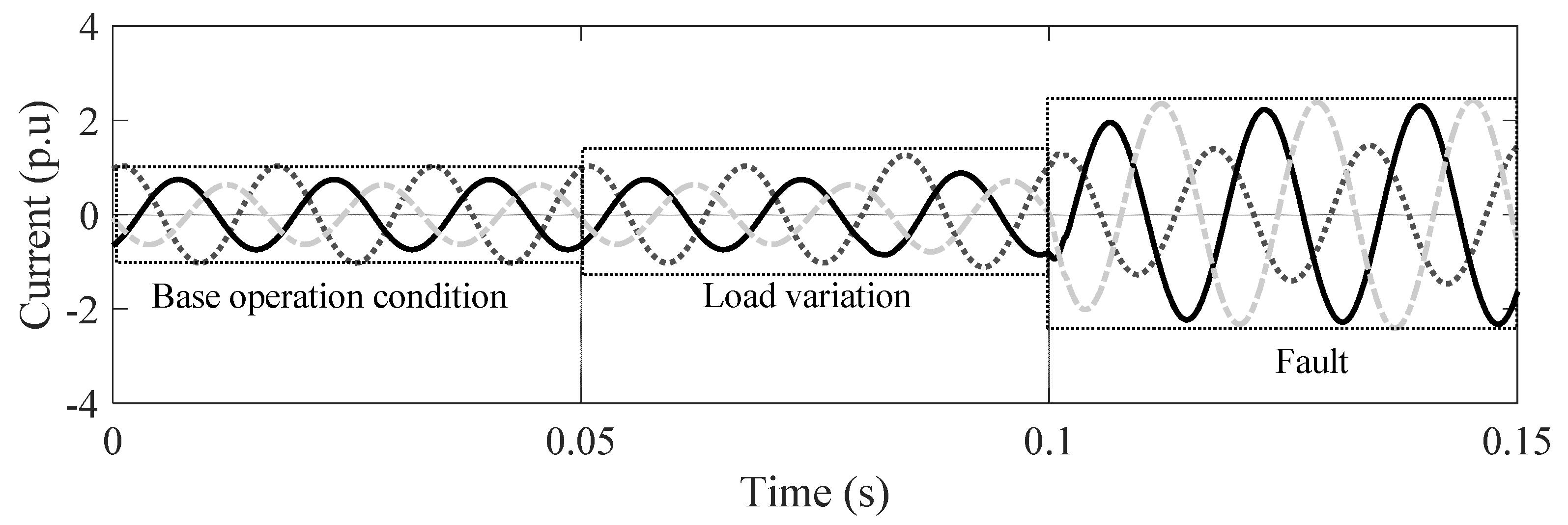
This change is carried out by creating a random load variation event in the EMT simulation of no more than 50% of the baseline operation condition. The third interval corresponds to the fault condition. The fault occurs at 0% and 50% of the line sections of the microgrid. The levels in Table 2 establish the fault resistance values. For this research, a simulation time of 150 ms was considered, where the random load variation event and fault event occurred at 50 ms and 100 ms, respectively. These intervals were selected as being long enough to avoid any transitory effects but short enough to allow for fast response of the protection devices. Figure 4 illustrates the current signal recorded by an IED under the above conditions, and the sampling frequency was set to 10 kHz.

• Stage 3: Database labeling

During the previous stage, for each simulated operation scenario, the V and I signals are obtained at the installation points of each IED. In this new stage, the resulting V and I signals are labeled as follows:

✓

Non-faulted: this class includes all normal operation condition scenarios of the microgrid. This scenario is labeled as class 1 in this work.

✓

Fault condition without relay activation: this class includes all fault events that can be detected by the IED but did not occur in its protection zone. This scenario is labeled as class 2 in this work.

✓

Fault condition with relay activation: this class includes all fault events that occur in the protection zone of each IED.

2.2. Stage II: Input Data Adjustment

The definition and selection of attributes is a critical process in the application of ML techniques. The features should be selected, seeking to maximize the amount of information that they capture from the database [13]. Additionally, if a lower number of attributes is employed, the dimensionality of the problem space is also reduced, which can improve the performance of ML techniques on a given dataset [39]. Several attributes for FD approaches have been proposed in [13,21,22,23,26,40]. In this work, the 49 attributes listed in

Table 3. Definition and estimation of attributes.

Attribute	Estimation	Number of Features	References
Root mean square (RMS) voltage and current signal $(V_a,V_b,V_c,I_a,I_b,I_c)$	$x_{rms}=\sqrt{{\displaystyle {\displaystyle \sum }_{k=0}^{N-1}}\raisebox{1ex}{$X_k^2$}\!\left/ \!\raisebox{-1ex}{$2$}\right.}$	6	[13,22,36,40,41]
Phase angle $({\theta }_{va},{\theta }_{vb},{\theta }_{vc},{\theta }_{ia},{\theta }_{ib},{\theta }_{ic})$	${\phi }_X=\max \left(angle(X_k)\right) k=0,\dots , N-1$	6
Frequency $(f)$	$f=f_k | X_k=\max (X_k) k=0, \dots , N-1$	1
Active and reactive power $(P_a,P_b,P_c,Q_a,Q_b,Q_c)$	$S=P+jQ=V_{rms}{I}_{rms}\left(\cos ({\phi }_V-{\phi }_I)+j\sin ({\phi }_V-{\phi }_I)\right)$	6
Mean of the fundamental frequency contours $(m{V}_a,m{V}_b,m{V}_c,m{I}_a,m{I}_b,m{I}_c)$	$\overline{x}={\displaystyle {\displaystyle \sum }_{m=0}^N}\frac{X_{(m,{\omega }_o)}}{N}$	6	[25,30,35,36]
Standard deviation of the fundamental frequency contours $(std{V}_a,std{V}_b,std{V}_c,std{I}_a,std{I}_b,std{I}_c)$	$S=\sqrt{\frac{1}{N}{\displaystyle {\displaystyle \sum }_{m=0}^N}{\left(X_{(m,{\omega }_o)}-\overline{x}\right)}^2}$	6	[23,32,33,35]
Entropy of the fundamental frequency contours $(S{V}_a,S{V}_b,S{V}_c,S{I}_a,S{I}_b,S{I}_c)$	$H\left(X_{(m,{\omega }_o)}\right)={\displaystyle {\displaystyle \sum }_{m=0}^N}p(X_{(m,{\omega }_o)}){\log }_{2}p(X_{(m,{\omega }_o)})$	6	[32,33,35]
Kurtosis of the fundamental frequency contours $(kt{V}_a,kt{V}_b,kt{V}_c,kt{I}_a,kt{I}_b,kt{I}_c)$	$Kt\left(X_{(m,{\omega }_o)}\right)=\frac{{{\displaystyle \sum }}_{m=0}^N{\left(X_{(m,{\omega }_o)}-\overline{x}\right)}^4}{N{S}^4}-3$	6
Obliquity of the fundamental frequency contours $(sk{V}_a,sk{V}_b,sk{V}_c,sk{I}_a,sk{I}_b,sk{I}_c)$	$Kt\left(X_{(m,{\omega }_o)}\right)=\frac{1}{N}\frac{{{\displaystyle \sum }}_{m=0}^N{\left(X_{(m,{\omega }_o)}-\overline{x}\right)}^3}{S^3}$	6

were used. These attributes were computed for each signal cycle, taking approximately 160 samples to describe a 60 Hz cycle.

It is possible that two or more of these attributes are highly correlated. Therefore, a selection method must be used to determine the most representative attributes.

2.3. Stage III: Parametrization and Training of ML Techniques

This stage is composed of three steps: the selection of the ML technique, selection of representative attributes, and parametrization and training. The processing steps are explained in Section 2.3.1, Section 2.3.2 and Section 2.3.3.

2.3.1. Step 4: Selection of the ML Technique

Three ML algorithms are considered, choosing among them by finding the best overall performance when each algorithm is tuned using a heuristic adjustment of its hyper-parameters. For this approach, the value of each hyper-parameter is varied between a range until the performance of the corresponding technique reaches its peak. This process was carried out considering the 49 attributes from stage 2. The ML techniques considered for this work were random forest (RF), support vector machine based on radial basis function kernel (SVM), and K-nearest neighbors (K-NN), which are commonly used in the literature to solve fault detection problems.

Table 4. Machine learning (ML) techniques and hyper-parameters.

ML Technique	Hyper-Parameter	Interval
Random forest classifier (RF)	Threshold selection	Gini, entropy.
	Number of trees	$(0-20)$
K-nearest neighbors (K-NN)	Number of neighbors	$(0-20)$
Support vector machine (SVM)	C factor	$(0-20)$
	Gamma factor	$(0-20)$

shows the hyper-parameters for each ML technique and the intervals considered for tuning [42].

2.3.2. Step 5: Determination of Representative Attributes.

In this step, the number of features that represent the largest amount of database information are selected, reducing problem space dimensionality and computational requirements. For this research, two feature selection techniques were used [43]:

• Principal component analysis (PCA)

PCA is a complexity reduction technique used for the analysis of intrinsic database variability [44]. This technique uses a transformation to gain new attributes, called components, on the basis of the original features, maximizing variance and minimizing the lineal correlation between features. In order to diminish the loss of information in the transformation process, PCA employs the covariance matrix for transforming a database Xn x m in a database Yn x l such that $l\ll m$. This method is given by Equation (1).

$$X={\displaystyle \sum }_{a=1}^l{t}_a{p}_a^T+E | X \in R^{mxn} \Lambda l\le n$$

(1)

where $X$ is the set of data to be analyzed by principal components, $l$ is the number of components, $p_a$ is an orthonormal vector that contains the relationship between the features, and $t_a$ is the projections of X over $p_a$. Finally, $E$ is the error of the model. Therefore, given Equation (1), the PCA is placed on the decomposition in eigenvalues of the covariance matrix $cov(X)=X^{T}X/(n-1)$.

The new features are selected on the consideration that their contribution is more than 1% of the database variation and that their combination with other features represents at least 98% of the total data variation.

• Singular value decomposition (SVD)

Algebraically, any matrix X can be divided into a linear combination of matrixes with rank 1, which is described by Equation (2) [45].

$$X={\displaystyle \sum }_{i=1}^m{u}_i{\sigma }_i{v}_i^T | X \in R^{mxn}, u\in R^{mxm} , \sigma \in R^{mxn}, v \in R^{nxn}$$

(2)

where $u$ and $v$ are orthonormal matrices, and $\sigma$ is a diagonal matrix with non-negative values, which are called singular values. A way to obtain these from a matrix is through the eigenvalues ${\lambda }_i$ of the square matrix $A=X{X}^T$, such that the singular value ${\sigma }_i$ meets the condition ${\sigma }_i=\sqrt{{\lambda }_i}$.

As is the case with the PCA method, the SVD saves the relevant information for each dimension of a database. With this information, it is possible to determine the number of attributes that can describe the original database efficiently. As a disadvantage, both Principal component analysis (PCA) and SVD result in new abstract feature spaces generated by combining features in the original space.

2.3.3. Step 6: Parametrization and Training of ML Techniques

The parametrization and training processes are performed simultaneously in this step. As in step 5, the ML technique is selected and its hyper-parameters are estimated, and the parametrization process is addressed in order to determine the combination of the features that maximize the performance of the ML technique computed using cross-validation. Cross-validation is a procedure for determining the ML performance through the training database being divided into N subsets (folds), and N models are trained and tested using a leave-one-out scheme [46]. The overall performance is computed as the average of the accuracy of the N resulting models. For the case presented here, the number of feature combinations was 249. Therefore, to determine the feature combination that maximizes the performance of the ML technique is not a trivial task. That is why a Chu–Beasley genetic algorithm (CBGA) was implemented to achieve this goal. Figure 5 presents each stage of the CBGA, and the next sections explain in detail each stage [47].

• Stage 1: Generation of the initial population

The CBGA is a computer simulation in which a population of abstract representations (genotype of the genome) of solution candidates (individuals or chromosomes) to an optimization problem is modified through an evolutionary mechanism that results in a trend towards better solutions [48]. For the fault detection problem, an initial population of 20 individuals is used, where each individual is composed by 49 chromosomes that represent each electrical attribute. Each chromosome can take the value of zero (0) or one (1): zero indicates that the electrical feature obtained in step 3 is not considered, and 1 that this is considered in the combination of attributes defined by the individual. Additionally, an infeasibility function is implemented to limit the number of features for each chromosome. The maximum number of features is determined by the techniques presented in step 5. Additionally, each chromosome is qualified through a fitness function, which is computed as the performance of the ML model when trained on the features defined in the chromosome.

• Stage 2: Making of next generation

In this process, new generations of individuals are obtained from the crossing of the individuals that compose the current population. This is achieved through three evolution mechanisms as shown in Figure 5. The selection of parents is carried out by tournament, where two groups composed of five individuals of the current population are randomly selected, such as the individual with the highest performance being selected from each group. With the definition of the two parents, the crossing between them is generated using a selected crossover. For this, two random numbers between 0 and the length of the individual are obtained, exchanging the part of the chromosome that is between these two values. From this process, two new individuals called children are obtained, but only one is chosen randomly for the next generation [49]. The third evolution mechanism is the mutation. For this process, a random number from 0 to 1 is found. If the number is greater than 0.85, the genome of a random chromosome is changed so that if the genome is 1, this is changed to 0.

• Stage 3: Decision criterion

Considering the coding strategy used in the approach, the new descendent could substitute the individual who has the worst objective function if, and only if, the descendent has a better objective function and meets the diversity criterion. This is achieved through three decision criteria. The first corresponds to the feasibility criterion, which determines if the number of features defined by the current chromosome is less than the number of representative features selected in step 5. The second criterion corresponds to the aspiration criterion, where if the performance of the current descendent is lower than the fitness of any chromosome of the current population, and then a number of mutations are applied in order to improve their fitness. Finally, the third criterion corresponds to the selection criteria. This determines whether the new descendent replaces an individual in the current population. The replacement is carried out if, and only if, there is an unfeasible chromosome in the current population, or if the child chromosome has better performance than the worst individual in the population and is less infeasible than the individual being replaced. In cases of gaining better performance and major infeasibility, it replaces the most infeasible.

Stages 2 and 3 are performed until a defined number of iterations is reached, or the accuracy change rate between the parents is less than 1%. As a result of step 7, the ML model for each IED with the best performance reported in the training process is obtained, obtaining a combination of 16 features in the worst-case scenario, thus reducing the ML model complexity.

2.4. Stage IV: Validation of ML Techniques

Step 7: Performance of the ML Techniques

In order to validate the ML models determined in step 2.3, their performance was studied using a test database, which corresponded to 15% of the database that was not considered in the training process.

3. Case Study

The proposed method was validated on the modified IEEE 13-node test feeder [50]. This feeder operates at a voltage of 24.9 kV and is characterized by being short and relatively highly loaded, and having overhead and underground lines, shunt capacitors, an in-line transformer, and unbalanced loading. This system was modeled in the DIgSilent Power Factory simulation software and modified by inserting one photovoltaics source (PV) system of 1.5 MW, a conventional synchronous generator of 2 MW, and one wind generator of 1MW. Figure 6 presents the IEEE 13-node test feeder.

4. Validation and Discussion

The validation of the proposed FD system was carried out by its implementation on the case study and the sensitivity analysis. Section 4.1 and Section 4.2 present the obtained results and discussion for the application of each stage of FD system and sensitivity analysis.

4.1. FD System Implementation

Section 4.1.1, Section 4.1.2, Section 4.1.3 and Section 4.1.4 present the implementation of each stage of FD system.

4.1.1. Stage I: Database from Simulations

The database from simulations was obtained by simulating the possible operating scenarios of the microgrid. These scenarios were obtained from its operation modes (on-grid/off-grid) and three reference load conditions defined as low-load condition, half-load condition, and nominal-load condition, as presented in

Table 5. Operational condition of microgrid.

Scenario	Operation Mode	Reference Load Condition
1	On-grid	Low load: 30% of nominal load.
2		Medium load: 70% of nominal load.
3		High load: nominal values.
4	Off-grid	Low load: 30% of nominal load.
5		Medium load: 70% of nominal load.
6		High load: nominal values.

.

Table A1. Spot Load Data.

Node	Load	Ph-1	Ph-1	Ph-2	Ph-2	Ph-3	Ph-3
	Model	kW	kVAr	kW	kVAr	kW	kVAr
634	Y-PQ	160	110	120	90	120	90
645	Y-PQ	0	0	170	125	0	0
646	D-Z	0	0	230	132	0	0
652	Y-Z	128	86	0	0	0	0
671	D-PQ	385	220	385	220	385	220
675	Y-PQ	485	190	68	60	290	212
692	D-I	0	0	0	0	170	151
611	Y-I	0	0	0	0	170	80
	TOTAL	1158	606	973	627	1135	753

,

Table A2. Distributed Load Data.

Node A	Node B	Load	Ph-1	Ph-1	Ph-2	Ph-2	Ph-3	Ph-3
		Model	kW	kVAr	kW	kVAr	kW	kVAr
632	671	Y-PQ	17	10	66	38	117	68

and

Table A3. Random variation load.

Load Condition	Values
Low–medium load condition	30–48%
Medium–nominal load condition	70–102%
Nominal–high load condition	100–147%

of the Appendix A show the load values used in the generation of the database.

Several factors for generation of the normal operation conditions and faulted conditions were used.

Table 6. Factors and level for case study.

Group	Factors for Case Study	Levels for Case Study	Number of Operation Conditions
No-fault operation	Random load variation	(0–50%)	23,606
	Topology change	Scenario 1 to 6
	Cut off generation	Without cut off generation Cut off PV generator Cut off wind generator
Fault operation	Fault type	A-g, AB, and ABC	23,606
	Fault location	All the lines of the system
	Fault resistance	(0–50 Ω)
	Fault position	0–50%
	Random load variation	(0–50%)
	Topology change	Scenario 1 to 6

presents the factors used in this stage. For each group (normal condition and faulted-condition), 23,606 scenarios were obtained, because the theory of the ML recommends that each class has the same number of scenarios so as not to bias the technique performance [51]. For each scenario, voltage and current signals at the installation points of the IEDs were obtained. The location of the IED is illustrated in Figure 6. Additionally, the labeling process mentioned in Section 2.1.2 was also carried out. As a result of this stage, a database from simulations composed of the voltage and current signals at the installation points of the IED were obtained.

4.1.2. Stage II: Input Data Adjustment

In this stage, the 49 attributes defined in Section 2.2 were estimated for each scenario obtained in stage 1. In addition, the randomization of the database was generated by using a random Python function that returns uniformly distributed pseudorandom numbers [52]. The number of cases selected for the validation process was 7080.

4.1.3. Stage III: Parametrization and Training of ML Techniques

The parameterization process was carried out in the three steps mentioned in Section 2.3. The following sections present their application to the case study.

• Selection of the ML technique

Three classic ML techniques were used in the proposed methodology for the case study: random forest (RF), support vector machine (SVM), and K-nearest neighbors (K-NN). The selection of the ML technique was carried out by heuristic adjustment of its hyper-parameters to gain an improvement in its performance, as presented in Section 2.3.1. The performance of the techniques was given by accuracy, as defined by Equation (3).

$$Ac=\frac{TF+TFW+TNF}{TF+TFW+TNF+FF+FFW+FNF}$$

(3)

where TF is the number of operation conditions that are true under fault; TFW is the number of operation conditions that are true in fault with activation; TNF is the number of operation conditions that are true under no-fault; FF is the number of operation conditions that wrongly predicted a fault; FFW is the number of operation conditions that wrongly predicted a fault with activation, and FNF is the number of operation conditions that wrongly predicted a no-fault.

For this process, the 49 attributes for each database scenario were considered. In the next section, the performances for each ML technique in function of adjustment of their hyper-parameters are presented. These processes are executed for each IED, taking into account the validation dataset.

○

Support vector machine (SVM)

This SVM used a radial basis function kernel, which had two hyper-parameters, $C$ and $\gamma$. To assess the effect of each hyper-parameter individually, one of them was set to 1 and the other hyper-parameter was varied according to the interval of Table 4. Figure 7 shows the behavior of the accuracy of the SVM technique when the hyper-parameters were varied independently.

From Figure 7a,b, it can be observed that ML technique performance improved for all IED as the hyper-parameters increased. However, there was a zone where the increase of the hyper-parameter did not produce an improvement in performance. Hyper-parameters must be adjusted near this zone to avoid overfitting.

○

Random forest (RF)

For random forest, the Gini criterion was selected to minimize the probability of misclassification. Therefore, the hyper-parameter to be adjusted was the number of trees. Figure 8 shows the behavior of the accuracy of the RF technique when the number of trees was modified.

Similar to the previous case, Figure 8 shows that if the number of trees was increased, a slight increase in accuracy was obtained. However, as the number of trees increased, this improvement tended to be negligible. The above occurred for a number of trees greater than eight, where the accuracy for relays was greater than 90% for RF technique evaluated. The best performance was achieved for relays 1 and 10. The good performance of relay 1 was probably related to the fact that it acted for all faults in on-grid connected mode, whereas in the off-grid mode, it should not detect faults. On the other hand, relay 10 only discriminated the faults that occurred in its line segment.

○

K-nearest neighbors (K-NN)

The performance of the K-NN technique in function of adjustment of its hyper-parameters was obtained. In this case, the hyper-parameter was the K neighbors. Figure 9 presents the behavior of the accuracy of this technique when the number of K neighbors was modified.

For the K-NN technique, the performance decreased for all IED as the hyper-parameters increased. To avoid overfitting problems, the hyper-parameter should be adjusted to a small number of neighbors. For this technique, the number of neighbors’ K was set to 3. Note that it is possible to achieve accuracies greater than 87% for all relays regardless of K value. The accuracy for relays 1 and 10 was similar to that presented in Figure 8. This supports the assumption that the allocation of these relays influences their performance.

○

Hyper-parameter setting for each ML technique

From the results obtained in Figure 7, Figure 8 and Figure 9, the adjustment values of the hyper-parameters were selected by applying an exponential smoothing technique to each curve and taking their inflection point. These values were approximated to the nearest integer value, and the value that was repeated more often was taken as the hyper-parameter setting. The hyper-parameter setting for each ML technique is presented in

Table 7. Hyper-parameter setting and accuracy for each ML technique.

ML Technique	Hyper-Parameter	Value	Accuracy
RF	Number of trees	8	>90%
SVM	[γ,C]	[5,6]	>80%
K-NN	Number of neighbors	3	>85%

.

○

Comparison and selection of the ML technique

Table 7 shows that the best performing technique for the cases evaluated was RF. Additionally, the ML models obtained with this technique are easy to implement. For these reasons, RF was selected in this work.

• Selection of representative attributes

The selection of representative attributes was carried out by means of PCA clustering and SVD clustering techniques, as presented in Section 2.3.2.

Table 8. Number of representative attributes.

Device	Number of Representative Attributes	Information PCA (%)	Number of Representative Attributes	Information SVD (%)
R1	18	99.25	16	99.76
R2	16	99.12	17	99.67
R3	17	98.74	18	99.52
R4	16	99.32	16	98.43
R5	16	99.85	16	99.22
R6	19	99.38	18	99.55
R7	17	99.8	16	98.97
R8	19	99.1	18	99.12
R9	16	99.27	16	99.55
R10	16	98.82	19	99.9

presents the number of representative attributes determined by each technique for each system relay. Additionally, it shows the percentage of information that represents the number of attributes.

Table 8 shows that the combination of 16 features can represent more than 98% of the information of the database. Therefore, 16 was selected as the maximum number of representative features. The above represents a significant reduction of attributes (from 49 to 16), which reduces the computational effort and the presenting of data scarcity [53].

• Parametrization and training of ML techniques

Once the maximum number of representative attributes was determined, a Chu–Beasly genetic algorithm was used in order to determine the combination of attributes that maximize the performance of the ML technique. Section 2.3.3 presents the formulation of the algorithm used. The results obtained for each relay with its combination features and accuracy are shown in

Table 9. Training and validation results.

Relay	Attributes Combination	Accuracy (%)
		Training	Validation
R1	$std{V}_b,I_a,{\theta }_{ia},sk{I}_a,I_b,m{I}_b,std{I}_b,kt{I}_b,{\theta }_{ic},Q_c$	96.6553	96.4548
R2	$m{V}_a,std{V}_a,m{V}_b, kt{V}_c,I_a,{\theta }_{ia},sk{I}_a,{\theta }_{ib},I_c,{\theta }_{ic},m{I}_c$	96.8207	96.4548
R3	$V_a,{\theta }_{va}, std{V}_a,V_b,sk{V}_b,V_c,S{V}_c,m{I}_a,S{I}_a,kt{I}_b,P_b,P_c$	97.1745	96.7796
R4	$m{V}_a,V_b, sk{V}_b,V_c,I_a,m{I}_a, kt{I}_a,I_c,{\theta }_{ic},P_a$	98.7218	98.5593
R5	$std{V}_a, sk{V}_a,kt{V}_a,m{V}_b, {\theta }_{vc},std{V}_c,I_a,I_b,m{I}_b,sk{I}_b,I_c,P_a$	99.1528	99.8587
R6	$std{V}_a, V_b, std{V}_b,sk{V}_b,kt{V}_b,V_c, I_a,kt{I}_a,{\theta }_{ia},I_b,kt{I}_b,I_c,P_b,Q_c$	95.8789	95.7062
R7	$std{V}_a, V_b, std{V}_c,sk{V}_c,kt{V}_c, I_a,I_b,{\theta }_{ib},P_c$	97.7650	97.9519
R8	$V_b, std{V}_c, I_a,m{I}_a,I_b,{\theta }_{ib},{\theta }_{ic},std{I}_c,kt{I}_c,Q_a,P_c,Q_c$	99.8754	99.8446
R9	$sk{V}_a, V_a, kt{V}_a,m{V}_b,std{V}_c,sk{V}_c,sk{I}_a,I_c,P_c$	100	100
R10	$sk{V}_a, m{V}_b, std{V}_c, I_a,std{I}_a,S{I}_a,kt{I}_a,I_b,I_c,{\theta }_{ic},sk{I}_c,P_a,Q_c$	99.9177	99.8870

.

These results showed high accuracy of the model obtained in the training process. However, it was necessary to determine the accuracy for events that were not used in the parameterization and training process, which is presented in Section 4.1.4.

4.1.4. Stage IV: Validation

• Step 7: Performance of the ML techniques

To validate the performance of the training models obtained in stage III, the 15% of the database generated in stage I, and that which was not used in the training process was considered. This validation considered all factors presented in Table 6. Additionally, in order to guarantee the statistical validity of the experiment, the proposed FD system was executed 30 times for the tests evaluated. Table 9 shows the accuracy of the ML models for each relay validated.

The results obtained showed satisfactory performance of the proposed FD system, presenting an accuracy greater than 95% for all cases evaluated. Although similar performances were reported in [22,23,25,26,27,28,29,30], in this work, a strategy to select the ML technique, the representative features, and their combination in order to optimize the performance of proposed FD technique were formulated. Additionally, all the stages were presented with enough detail for their understanding and replication, which is not usually observed in the FD state-of-the-art techniques.

However, these tests do not allow for the determination of the factors that affect most the performance of the FD system. In consequence, a sensitivity analysis was performed, as presented in the following section.

4.2. Sensitivity Analysis

In order to know the factors that directly affect the performance of the proposed FD system, a sensitivity analysis by an experimental design was executed. This was composed of a set of five factors, which are presented in

Table 10. Factors for the sensitivity analysis.

Factors	Levels	Scenarios
Ft: Fault type	Single line to ground fault—double line fault—double line to ground fault three-phase fault	4
Fp: Fault position	0%, 50%	2
Ld: Load condition	(30–45%), (70–105%), (100–150%)	3
Gc: Grid connection	Ongrid/offgrid	2
RL: Relay location	R1, R2, R3, R4, R5, R6, R7, R8, R9, and R10	10

. For each level, 600 repetitions were executed in order to guarantee the statistical validity of the experiment.

According to the factors, levels, and the number of repetitions, the total number of experiments was 28,800, obtained by $TNE=r{{\displaystyle \prod }}_{i=1}^n{n}_i$ where $r$ is the number of repetitions and $n_i$ is the number of levels of the factor $i$. Each experiment was represented with the accuracy obtained after each trained model was tested with the validating signals that described the experiment.

The homogeneity between all the populations that were described by the level combinations was validated by the sensitivity analysis. The above was achieved through the following hypothesis test:

$$\begin{gathered} H_o: {\mu }_i={\mu }_j \forall i\ne j \\ {H}_1: {\mu }_i\ne {\mu }_j at least one i \end{gathered}$$

(4)

where i represents the level combination that has a different mean in case the null hypothesis was rejected [54].

An analysis of variance ANOVA was selected as a way to refuse the null hypothesis. ANOVA residues were employed to verify accomplishment with the normality, independence, and homoscedasticity criteria. The above is shown in Figure 10. In addition, statistical testds such as Jarque–Bera, Durbin–Watson, and Levene were executed as another way to confirm ANOVA assumptions.

The p-values of the statistical tests Jarque–Bera, Durbin–Watson, and Levene were 0.0945, 0.3395, and 0.2642, respectively. For all the tests, the p-values were higher than 0.05. Therefore, the assumptions of normality, homoscedasticity, and independence were validated, and the ANOVA results were truthful.

The results of the ANOVA are presented in

Table 11. ANOVA for each factor.

Source Principal Effects	SS	df	F-Ratio	p-Value
A: Fault type	0.005494	1	1.21504	0.2704
B: Fault position	0.105922	1	234.248	7.96 × 10−51
C: Load behavior	5.312 × 10−5	1	0.11749	0.731796
D: Grid connection	0.029042	1	64.2281	1.6166 × 10−15
E: IED location	0.089770	1	198.529	1.3463 × 10−43

. Factors with p-values greater than 0.05 were considered not statistically significant for the model studied.

The above occurred for factors A and C: fault type and load behavior, respectively. Therefore, it is possible to reject that these factors had an influential factor in the sensitivity of the proposed FD system. The above follows the shown behaviors, where each IED was composed of different feature combinations and presented different behavior with respect to the hyper-parameters of the techniques. On the other hand, it was expected that a grid connection such as the fault position had a statistical dependence because this incident affected the protection configuration directly.

5. Conclusions

This paper presented an intelligent fault detection system for microgrids. The obtained results showed a satisfactory performance, with an accuracy greater than 95.7% for the cases evaluated, although only voltage and current measurements registered locally by IED were used and the need for communication systems for the protection process was eliminated.

Additionally, the intelligent FD system presented a methodology composed of four steps that allowed for its implementation on any microgrid. From these steps, the database from simulations generating the process of micro-network operation and parameterization was highlighted.

The database-generating process presented recommendations for the generation of a high-quality database, which would guarantee the success of the use of ML models. The parameterization process showed how to determine the number of representative attributes that represent the largest amount of information in the database, which is valuable in order to reduce computational effort and avoid the presence of data scarcity. In addition, in the same parameterization process, a Chu–Beasley genetic algorithm was used to determine the best combination of attributes that would maximize the performance of ML techniques. Finally, the technique presented performances greater than 95% in both the training and validation process, and the sensitivity analysis showed that factors such as the fault type and load condition did not affect the performance of the proposed fault detection system, whereas other factors such as IED location were significant for the model. This implies that the training process must be executed on all available devices because, depending on this, the performance of the methodology might change.

Finally, we can summarize the main practical and economic benefits of employing the proposed FD system as being

• reduction of implementation cost because it does not need a communication system to FD process;
• diminishment of computational effort by the implementation of PCA, SVD, and Chu–Beasley techniques to reduce of number of features;
• consideration of the main operation condition scenarios in the microgrid, such as connected/islanded mode of the grid, cut-off/cut-on generation, network imbalance, and changes in topology, which reduce the probability of mis-operation in the protection scheme.

References

- Akorede, M.F.; Hizam, H.; Pouresmaeil, E. Distributed energy resources and benefits to the environment. Renew. Sustain. Energy Rev. 2010, 14, 724–734. [Google Scholar] [CrossRef]
- Chowdhury, S.; Chowdhury, P. Crossley Microgrids and Active Distribution Networks; The Institution of Engineering and Technology: London, UK, 2009; ISBN 9781849190145. [Google Scholar]
- Das, R.; Kanabar, M.; Adamiak, M.; Apostolov, A.; Antonova, G.; Brahma, S.; Zadeh, M.D.; Hunt, R.; Jester, J.; Kezunovic, M.; et al. Advancements in Centralized Protection and Control Within a Substation. IEEE Trans. Power Deliv. 2016, 31, 1945–1952. [Google Scholar]
- Huang, W.T.; Yao, K.C.; Wu, C.C. Using the direct search method for optimal dispatch of distributed generation in a medium-voltage microgrid. Energies 2014, 7, 8355–8373. [Google Scholar] [CrossRef]
- Atia, R.; Yamada, N. Distributed renewable generation and storage system sizing based on smart dispatch of microgrids. Energies 2016, 9, 176. [Google Scholar] [CrossRef] [Green Version]
- Hatziargyriou, N. Microgrids: Architectures and Control; John Wiley & Sons: London, UK, 2013; ISBN 9781118720677. [Google Scholar]
- Mariam, L.; Basu, M.; Conlon, M.F. Microgrid: Architecture, policy and future trends. Renew. Sustain. Energy Rev. 2016, 64, 477–489. [Google Scholar] [CrossRef]
- Kuo, M.T.; Lu, S. Der Design and implementation of real-time intelligent control and structure based on multi-agent systems in microgrids. Energies 2013, 6, 6045–6059. [Google Scholar] [CrossRef]
- Gers, J.M.; Holmes, E.J. Protection of Electricity Distribution Networks; IET: London, UK, 2011; ISBN 9781849192231. [Google Scholar]
- PSrivastava, A.; Parida, S.K. Frequency and Voltage Data Processing Based Feeder Protection in Medium Voltage Microgrid. In Proceedings of the 2019 IEEE PES Innovative Smart Grid Technologies Europe (ISGT-Europe), Bucharest, Romania, 29 September–2 October 2019; p. 5. [Google Scholar]
- Bansal, Y. Microgrid Fault Detection Methods: Reviews, Issues and Future Trends. In Proceedings of the 2018 IEEE Innovative Smart Grid Technologies—Asia (ISGT Asia), Singapore, 22–25 May 2018; pp. 401–406. [Google Scholar]
- Habib, H.F.; El Hariri, M.; Elsayed, A.; Mohammed, O. Utilization of Supercapacitors in Adaptive Protection Applications for Resiliency against Communication Failures: A Size and Cost Optimization Case Study. In Proceedings of the 2017 IEEE Industry Applications Society Annual Meeting, Cincinnati, OH, USA, 1–5 October 2017; pp. 1–8. [Google Scholar]
- Tang, W.J.; Yang, H.T. DataMining and neural networks based self-adaptive protection strategies for distribution systems with DGs and FCLs. Energies 2018, 11, 426. [Google Scholar] [CrossRef] [Green Version]
- Golestan, S.; Savaghebi, M.; Beheshtaein, S.; Guerrero, J.M.; Cuzner, R. A Modified Secondary-Control Based Fault Current Limiter for Four-Wire Three Phase DGs. IEEE Trans. Ind. Electron. 2018, 66, 4798–4804. [Google Scholar]
- Mumtaz, F.; Bayram, I.S. Planning, Operation, and Protection of Microgrids: An Overview. Energy Procedia 2017, 107, 94–100. [Google Scholar] [CrossRef]
- Amir, S.; Askarian, H.; Hossein, S.; Sadeghi, H.; Razavi, F.; Nasiri, A. An overview of microgrid protection methods and the factors involved. Renew. Sustain. Energy Rev. 2016, 64, 174–186. [Google Scholar]
- Chen, Y.-X.; Yin, X.-G.; Zhang, Z.; Chen, D.-S. Analysis of an Adaptive Overcurrent Relay for Transmission and Distribution Lines. In Proceedings of the International Conference on Power Systems Transients–IPST, New Orleans, LA, USA, 28 September–2 October 2003; pp. 1–6. [Google Scholar]
- Mahat, P.; Chen, Z.; Bak-jensen, B.; Bak, C.L. A simple adaptive overcurrent protection of distribution systems with distributed generation. EEE Trans. Smart Grid 2011, 2, 428–437. [Google Scholar] [CrossRef]
- Núñez-Mata, O.; Palma-Behnke, R.; Valencia, F.; Mendoza-Araya, P.; Jiménez-Estévez, G. Adaptive Protection System for Microgrids Based on a Robust Optimization Strategy. Energies 2018, 11, 308. [Google Scholar] [CrossRef] [Green Version]
- Piesciorovsky, E.C.; Schulz, N.N. Fuse relay adaptive overcurrent protection scheme for microgrid with distributed generators. IET Gener. Transm. Distrib. 2016, 11, 540–549. [Google Scholar] [CrossRef]
- Kar, S. A comprehensive protection scheme for micro-grid using fuzzy rule base approach. Energy Syst. 2017, 8, 449–464. [Google Scholar] [CrossRef]
- Kar, S.; Samantaray, S.R.; Zadeh, M.D. Data-Mining Model Based Intelligent Differential Microgrid Protection Scheme. IEEE Syst. J. 2017, 11, 1161–1169. [Google Scholar] [CrossRef]
- Mishra, D.P.; Samantaray, S.R.; Joos, G. A combined wavelet and data-mining based intelligent protection scheme for microgrid. IEEE Trans. Smart Grid 2016, 7, 2295–2304. [Google Scholar] [CrossRef]
- Hooshyar, A.; Iravani, R. Microgrid Protection. Proc. IEEE 2017, 105, 1332–1353. [Google Scholar] [CrossRef]
- Kar, S.; Samantaray, S.R. Combined S-transform and data-mining based intelligent micro-grid protection scheme. In Proceedings of the 2014 Students Engineering and Systems, Allahabad, India, 28–30 May 2014; pp. 1–5. [Google Scholar]
- Mishra, M.; Rout, P.K. Detection and classification of micro-grid faults based on HHT and machine learning techniques. IET Gener. Transm. Distrib. 2018, 12, 388–397. [Google Scholar] [CrossRef]
- Hudananta, S.; Haryono, T. Study of overcurrent protection on distribution network with distributed generation: An Indonesian case. In Proceedings of the 2017 International Seminar on Application for Technology of Information and Communication (iSemantic), Semarang, Indonesia, 7–8 October 2017; pp. 126–131. [Google Scholar]
- Abdulwahid, A.H.; Wang, S. A novel approach for microgrid protection based upon combined ANFIS and Hilbert space-based power setting. Energies 2016, 9, 1042. [Google Scholar] [CrossRef]
- Yu, J.; Hou, Y.; Lam, A.; Li, V. Intelligent Fault Detection Scheme for Microgrids with Wavelet-Based Deep Neural Networks. IEEE Trans. Smart Grid 2019, 10, 1694–1703. [Google Scholar] [CrossRef]
- Gashteroodkhani, O.A.; Majidi, M.; Fadali, M.S.; Etezadi-Amoli, M.; Maali-Amiri, E. A protection scheme for microgrids using time-time matrix z-score vector. Int. J. Electr. Power Energy Syst. 2019, 110, 400–410. [Google Scholar] [CrossRef]
- Kavi, M.; Mishra, Y.; Vilathgamuwa, M. Morphological Fault Detector for Adaptive Overcurrent Protection in Distribution Networks with Increasing Photovoltaic Penetration. IEEE Trans. Sustain. Energy 2018, 9, 1021–1029. [Google Scholar] [CrossRef]
- Alexopoulos, T.; Biswal, M.; Brahma, S.M.; Khatib, M. El Detection of fault using local measurements at inverter interfaced distributed energy resources. In Proceedings of the 2017 IEEE Manchester PowerTech, Manchester, UK, 18–22 June 2017. [Google Scholar]
- Samantaray, S.R. A data-mining model for protection of facts-based transmission line. IEEE Trans. Power Deliv. 2013, 28, 612–618. [Google Scholar] [CrossRef]
- Kar, S.; Samantaray, S.R. Intelligent anti-islanding protection scheme for distributed generations. In Proceedings of the 2013 Annual IEEE India Conference (INDICON), Mumbai, India, 13–15 December 2013; pp. 1–5. [Google Scholar]
- Kar, S.; Samantaray, S.R. Multiple features based anti-islanding protection relay for distributed generations. In Proceedings of the 2014 International Conference on Smart Electric Grid (ISEG), Guntur, India, 19–20 September 2014; pp. 1–6. [Google Scholar]
- Kar, S.; Samantaray, S.R. Data-mining based comprehensive primary and backup protection scheme for micro-grid. In Proceedings of the IEEE Power, Communication and Information Technology Conference (PCITC), Bhubaneswar, India, 15–17 October 2015; pp. 505–510. [Google Scholar]
- Sushrut, A.S.; Vijay, S.D. System reconfiguration in microgrids. Sustain. Energy Grids Netw. 2019, 17, 100191. [Google Scholar] [CrossRef]
- Zhao, W.; Bi, X.; Wang, W.; Sun, X. Microgrid Relay Protection Scheme Based on Harmonic Footprint of Short-Circuit Fault. Chin. J. Electr. Eng. 2018, 4, 64–70. [Google Scholar] [CrossRef]
- Wu, X.; Zhu, X.; Wu, G.-Q.; Ding, W. Data Mining with Big Data. IEEE Trans. Knowl. Data Eng. 2014, 63, 331–333. [Google Scholar]
- Bernabeu, E.E.; Thorp, J.S.; Centeno, V. Methodology for a security/dependability adaptive protection scheme based on data mining. IEEE Trans. Power Deliv. 2012, 27, 104–111. [Google Scholar] [CrossRef] [Green Version]
- Pardeshi, C.P.; Jadhav, G.N. Data-mining-based intelligent anti-islanding protection relay for distributed generations. In Proceedings of the IEEE International Conference on Power, Control, Signals and Instrumentation Engineering (ICPCSI), Chennai, India, 21–22 September 2017; pp. 2496–2501. [Google Scholar]
- Henao, R.; Hurtado, J.E.; Castellanos, G. Selección de hiperparámetros en máquinas de soporte vectorial utilizando adaptación de matriz de covarianza. Sci. Tech. 2005. [Google Scholar] [CrossRef]
- Honeine, P. Online kernel principal component analysis: A reduced-order model. IEEE Trans. Pattern Anal. Mach. Intell. 2012, 34, 1814–1826. [Google Scholar] [CrossRef]
- Williams, L.J. Principal component analysis. WIREs Comput. Stat. 2010, 2, 433–459. [Google Scholar]
- Lathauwer, L.D.E.; Moor, B.D.E.; Vandewalle, J. A multilinear singular value decomposition. SIAM J. Matrix Anal. Appl. 2000, 21, 1253–1278. [Google Scholar] [CrossRef] [Green Version]
- Soekarno, I.; Hadihardaja, I.K.; Cahyono, M. A Study of Hold-out and K-Fold Cross Validation for accuracy of Groundwater modeling in Tidal Lowland Reclamation Using Extreme Learning Machine. In Proceedings of the 2014 2nd International Technology, Informatics, Management, Engineering & Environment, Bandung, Indonesia, 19–21 August 2014; pp. 228–233. [Google Scholar]
- Correa-Tapasco, E.; Mora-Florez, J.; Perez-Londono, S. Hybrid approach for an optimal adjustment of a knowledge-based regression technique for locating faults in power distribution systems. DYNA 2011, 78, 31–41. [Google Scholar]
- Passos, G.C.S.; Barrenechea, M.H. Genetic algorithms applied to an evolutionary model of industrial dynamics. EconomiA 2019, in press. [Google Scholar]
- Demidova, L.A.; Egin, M.M.; Tishkin, R.V. A self-tuning multiobjective genetic algorithm with application in the SVM classification. Procedia Comput. Sci. 2019, 150, 503–510. [Google Scholar] [CrossRef]
- Kersting, W.H. Radial distribution test feeders. In Proceedings of the 2001 IEEE Power Engineering Society Winter Meeting, Columbus, OH, USA, 28 January–1 February 2001; pp. 908–912. [Google Scholar]
- Correa-Tapasco, E.; Mora-Flórez, J.; Perez-Londoño, S. Performance analysis of a learning structured fault locator for distribution systems in the case of polluted inputs. Electr. Power Syst. Res. 2019, 166, 1–8. [Google Scholar] [CrossRef]
- Xu, L.; Jiang, C.; Wang, J.; Yuan, J.; Ren, Y. Information security in big data: Privacy and data mining. IEEE Access 2014, 2, 1151–1178. [Google Scholar]
- Karystinos, G.N.; Pados, D.A. On overfitting, generalization, and randomly expanded training sets. IEEE Trans. Neural Netw. 2000, 11, 1050–1057. [Google Scholar] [CrossRef]
- Montgomery, D.C. Design and Analysis of Experiments; John Wiley & Sons: London, UK, 2012; Volume 2, ISBN 0471316490. [Google Scholar]
Figure 1.
Intelligent electronic devices (IEDs) installed at each end point of the line section without a communication link. DER: Distributed energy resources.
Figure 2.
Flowchart for the proposed fault detection system for microgrids.
Figure 3.
Flowchart of stage 1: database from simulations.
Figure 4.
Generation of non-fault and faulted events in a current signal.
Figure 5.
Chu–Beasley algorithm for parametrization and training of ML techniques.
Figure 6.
Modified IEEE 13-node test feeder as a microgrid.
Figure 7.
Support vector machine (SVM) performance in function of adjustment of its hyper-parameters: (a) SVM performance when it was varied with Gamma factor with C = 1; (b) SVM performance when it was varied with C factor with .
Figure 8.
Random forest (RF) performance in function of adjustment of its hyper-parameters.
Figure 9.
K-nearest neighbors (K-NN) performance in function of adjustment of its hyper-parameters.
Figure 10.
ANOVA assumption tests for distribution test: (a) distribution test; (b) independence test.