Optimal Location of Fast Charging Stations for Mixed Traffic of Electric Vehicles and Gasoline Vehicles Subject to Elastic Demands


1
School of Transportation and Logistics, Dalian University of Technology, Dalian 116024, China
2
China Academy of Transportation Sciences, Beijing 100029, China
*
Author to whom correspondence should be addressed.
Energies 2020, 13(8), 1964; https://doi.org/10.3390/en13081964
Submission received: 23 March 2020
/
Revised: 13 April 2020
/
Accepted: 14 April 2020
/
Published: 16 April 2020
(This article belongs to the Special Issue Electric Systems for Transportation)
Abstract
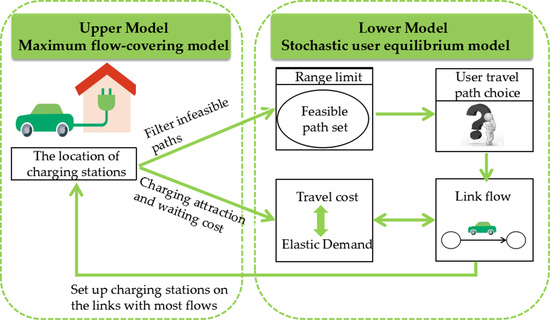
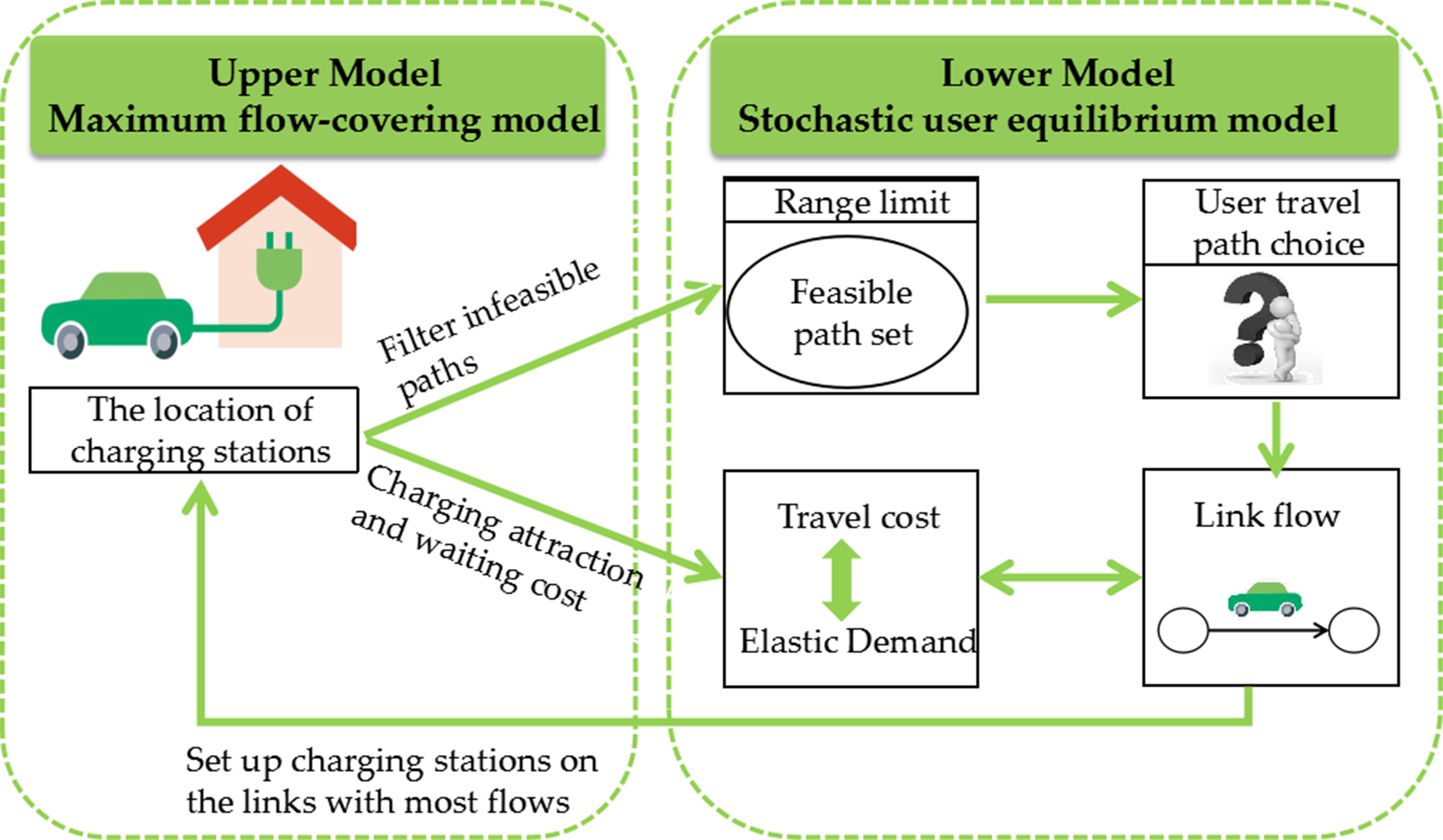
:With the rapid development of electric vehicles (EVs), one of the urgent issues is how to deploy limited charging facilities to provide services for as many EVs as possible. This paper proposes a bilevel model to depict the interaction between traffic flow distribution and the location of charging stations (CSs) in the EVs and gasoline vehicles (GVs) hybrid network. The upper level model is a maximum flow-covering model where the CSs are deployed on links with higher demands. The lower level model is a stochastic user equilibrium model under elastic demands (SUE-ED) that considers both demands uncertainty and perceived path constraints, which have a significant influence on the distribution of link flow. Besides the path travel cost, the utility of charging facilities, charging speed, and waiting time at CSs due to space capacity restraint are also considered for the EVs when making a path assignment in the lower level model. A mixed-integer nonlinear program is constructed, and the equivalence of SUE-ED is proven, where a heuristic algorithm is used to solve the model. Finally, the network trial and sensitivity analysis are carried out to illustrate the feasibility and effectiveness of the proposed model.
1. Introduction
The market share of new energy vehicles without fossil fuels has been increasing rapidly in recent years, especially electric vehicles (EVs), which provide better performance, higher efficiency, and zero emissions [1,2]. To promote the usage of EVs, governments around the world have successively issued a series of active policies to provide subsidies for EV purchases and to deploy public charging infrastructures at convenient locations [2,3]. However, the market acceptance of EVs seems to fluctuate with the decreasing subsidy. On the one hand, limited driving range, insufficient public charging infrastructures, and longer charging time are the main reasons for at-home charging. On the other hand, the deployment of EV charging stations may induce more trips [4,5], that is, demands between each origin to destination (OD) pair that respond to the available fast charging are elastic, so does the route choice. Therefore, it is especially important to study how to effectively and reasonably deploy EV public charging stations within the hybrid network of rapidly increasing EVs and dominated gasoline vehicles (GVs), which should help reduce the range anxiety of EV users and maximize the coverage rate of EVs.
According to previous studies, a variety of factors affect the location of charging stations, including, among others, preference and travel choice behavior of users [6,7], travel demand of users [8], information of the en-route energy consumption of EVs [9,10,11,12], information of the remained range of EVs [13,14], charging speed and demand of battery [7,15], road environment [5,16], land supply [17], elastic charging demands [18]. However, it is not practical to build a complicated location model and to solve the location problem by incorporating so many macro and micro factors into the planning and decision making of EV charging stations. This paper mainly studies the uncertainties due to the choice behavior of EV and GV users under elastic demands and uncertain path constraints. A bilevel model is proposed in this paper, where the upper model deals with a maximum flow-covering (MFC) problem, while the lower model is a stochastic user equilibrium model with elastic demands (SUE-ED). It is worth noting that factors, such as road congestion, charging speed, range limit of EVs, and capacity of charging stations, are already considered in users’ travel choices. The lower model considers the elastic demands and the distance constraints of EVs, which have a significant influence on route choice and the distribution of link flow. Finally, a generalized Lagrangian function is constructed to prove the equivalence between the stochastic user equilibrium model and the elastic demand model.
The remainder of this paper is structured as follows: Section 2 reviews the relevant literature. Section 3 affirms the problem hypothesis, analyzes three charging paths of the EVs, and gives the symbolic description used in the article. Section 4 establishes a bilevel model. Section 5 and Section 6 introduce the algorithms used to solve the model and numerical analysis applying to the Nguyen–Dupuis network, respectively. Finally, the research results and future research directions are discussed in Section 7.
2. Literature Review
The conventional and dominant three types of location optimization models include the point demand model [19,20], the flow demand model [20,21,22,23], and the multi-objective optimization model [24,25,26,27]. The P-Median model assumes that “charging demand is generated in the road network node” and is widely used as one of the point demand models. The flow demand model is formulated on the basis of the Flow Capturing Location Model (FCLM). For the first time, some researches proposed the Flow Refueling Location Model (FRLM), where mileage limitations were explicitly considered in facility location issues [28,29,30,31]. One branch of FRLM aims to maximize the demand coverage by locating a fixed number of charging facilities, which is called the maximum coverage location problem. Although the multi-objective optimization models have the advantage of addressing more complicated experimental requirements, they are not good at dealing with the uncertainty planning problem [32].
In a hybrid network with both EVs and GVs, the layout of EV charging stations and the distribution of EV flow affect mutually. Elastic demands in a hybrid network result in many more uncertainties. Most of the previous studies used the User Equilibrium Model (UE) to locate charging facilities. In these studies, Xu et al. dealt with the user equilibrium problem in a hybrid transport network with battery switching stations and road grade constraints [33]. Jing et al. gave a comprehensive discussion of the equilibrium network model [34]. Jiang et al. introduced the path distance constraints into the UE model [13]. Zheng et al. proposed a bilevel model where the upper layer minimized travel costs, and the lower layer aimed to find the path-constrained EVs equalization flow [35]. The bounded rationality of EV users led to much more complicated energy consumption [7,36,37], and, therefore, route choice behavior reflected more unobserved heterogeneity, which resulted in various elastic demands.
The network design problem with elastic demands, where the induced or transferred OD demand is the subject of responses in traveler itinerary choices to enjoy the improvement of new infrastructure, have several formulations with various motivations. Ge et al. [38] is one of the early attempts to consider both the proportion of EVs and the charge rate of EVs when determining the elastic charging demands from the total number of vehicles on road connections. The elastic demand was formulated based either on feedback of congested travel and congested station on route choices [39] or on the assumption that charge demand between OD pairs follows a nonlinear inverse cost function without considering the pre-generating paths and charging combinations [40].
It should be noted that it is hard to consider all these constraints simultaneously, say, the elastic demand of the road network, the capacity of the charging stations, and the range limit of EVs by using the SUE-ED model in location problems of public EV charging stations. In this study, a novel bilevel public charging station location model that combines a flow-capturing location model and a multi-objective optimization model is proposed.
3. Problem Assumptions and EV Paths Analysis
The proposed location model has two optimization objectives. The upper layer employs an improved maximum coverage model to maximize the coverage of the total EV flow by deploying a given number of charging stations on the links where the EV flow is the largest. The charging stations can serve more EV users by deploying charging facilities on the links where most EV drivers pass, which is an effective way to improve the utilization rate of public charging facilities and alleviate range anxieties of electric vehicle drivers [4]. The lower layer uses an SUE-ED model with incomplete information. The assignment result of SUE is a decisive factor for the placement of the charging stations. There is an inherent difference in the driving behavior of each user (EV users and GV users), in the hybrid network. In particular, range limit, charging time, and location of charging facilities have an important impact on the path choose behaviors of EV users.
3.1. Notations
i: The set of traveler types in the network. i presents an element, mainly including EVs and GVs. When specific instructions are needed, subscripts g and e are used to indicate variables or parameters related to GVs and EVs, respectively;
W: The set of OD pairs. w is an element of the set;
: The set of paths between all OD pairs;
p: The number of charging stations subject to the budget;
U: The utility value of the charging stations, resulting in a reduction in travel cost;
: The waiting cost in charging stations, where K is a constant coefficient;
: Length of path k between OD pair w;
: Length of path k between node r and I;
: Length of path k between node i and j;
: Length of path k between node j and s;
: The range limit of EVs;
ε: Charging power. Unit: hour/mile;
: The minimum charging time;
: Traffic flow on link a, including EVs and GVs, so
(,): Actual travel time through link a;
: Free travel time through link a;
: Capacity of link a;
: Binary parameter. If the charging facility is on link a, = 1, otherwise = 0;
: Binary parameter. If the path k crosses the link a, = 1, otherwise = 0;
: Elastic travel demand of type-i traveler between OD pair w;
: Maximum potential demand of type-i traveler between OD pair w;
: Traffic flow of type-i traveler on path k between OD pair w;
: The probability that type-i traveler chooses the path k between OD pair w;
: The actual travel time of the path k between OD pair w, and
: The generalized travel cost of type-i traveler on path k between OD pair w;
: The expected perceived travel cost of the type-i traveler between OD pair w;
(·): The traffic demand function of the type-i traveler between OD pair w;
: Vector of the actual travel cost of all paths between OD pair w;
: a non-negative parameter that characterizes the uncertainty of type-i traveler’s understanding of the path travel time.
3.2. Propose Assumptions
This paper focus on a hybrid network, denoted as G = (N,A), where N is the set of nodes, A is the set of links. W is used to represent a set of OD pairs, and w is an element, w ∈ W. represents the set of paths between w. The main differences between GVs and EVs are the limitation of travel distance and the composition of travel costs. Without loss of generality, the following assumptions are made:
- (a)
- There are two types of users in the mixed network: GVs and EVs, where EVs have an identical range limit;
- (b)
- The travel demand of GVs and EVs between each OD pair is elastic. And two types of vehicles have incomplete information about the travel cost;
- (c)
- Each EV is fully charged at its origin;
- (d)
- The level of anxiety and risk-taking behaviors of EV drivers are not considered in this model;
- (e)
- The charging time of electric vehicles is linearly related to mileage;
- (f)
- The charging facilities will be placed in the middle of links whose EV flow ranks p;
- (g)
- Deploying the charging facility on the road/path will increase the attractiveness of the route, which is called the utility of the charging facilities U, reducing the path travel cost;
- (h)
- Charging facilities have a fixed charging capacity. It is assumed that the waiting cost is proportional to the attraction value, expressed by .
3.3. Analysis of EV Paths
When performing SUE-ED traffic assignment, the GVs can choose any route because of no range limit. However, the selection of feasible path sets is required before the distribution of EV flow. To describe the three types of EV paths more clearly, the concept of sub-path is described as follows.
Suppose that the origin is r and the destination is s in a pair OD w, and there are two charging stations i, j, which are also regarded as nodes, located in the arc of the path k (Figure 1). When , , no longer includes other charging facilities except i, j, they are called sub-paths [41].
Based on the relationship between the travel mileage limit and the sub-path distance, the three travel paths of EVs are discussed, as shown in Table 1:
Scenario 1. A travel path that can be completed without charging. When ≤ , the EV drivers can reach the destination without charging. The generalized travel cost is (no charging stations) or (with charging stations).
Scenario 2. A travel path that cannot be completed after charging. When ≥ or or , the path k is an infeasible path. And the generalized path travel cost becomes infinite () and the probability that the drivers select the path is zero.
Scenario 3. A travel path that can be completed after charging. The path k is defined as a feasible path, if and ≤ and ≤ and ≤ . The drivers can complete the trip by charging at least once and the minimum charging time is = ε…(). The generalized travel cost is expressed as = = + + (K − 1)U, consisting of four parts: travel time, charging time, charging facilities utility, and charging stations’ waiting cost.
For GVs, the general path travel cost is = .
4. Establish a Double-Layer Model
In this section, a bilevel optimization model for the location of charging facilities is proposed. The upper level model determines the location of the charging facilities by selecting the top p links. The lower level model calculates users’ generalized travel cost, and randomly allocates the flow demand between the OD pairs to the filtered paths through known charging facilities location.
4.1. Upper Level Problem
The upper model is designed to maximize the total covered EV link flow by deploying a given number of charging facilities. The EV flow is covered when the charging facility is on the link. That is
Equation (1) is the objective function of the upper model, and Equation (2) is the budget constraint indicating the number of charging stations p in a given network.
4.2. Lower Level Problem
The Bureau of Public Road (BPR) function in the lower model is employed [42].
Since , , k are parameters that are independent of the equilibrium flow of the link, the Jacobian matrix [43] in the lower layer problem is as follows:
It proves that the Jacobian matrix is symmetrical, and the lower layer model can be established as a convex function problem. It is assumed that all types of travelers make path selection in a random manner. According to the random utility theory, the probability that type-i traveler chooses the path k between OD pair w is:
Assume that elastic travel demand of type-i traveler is a strictly monotonically decreasing function of the expected minimum travel time between OD pair w, and with an upper bound.
For the type-i traveler, its SUE condition can be expressed as:
In the mixed network, SUE-ED problem can be described by the equivalent mathematical programming model:
Equation (10) is the flow conservation constraint. Equation (11) is the non-negative constraint of path flow for type-i travelers. Equation (12) is the non-negative constraint of type-i traveler’s OD flow demand. Equation (13) is the correlation between link flow and path flow. The novelty of this problem is that the introduction of sub-paths in the Equation (14) can generate a feasible set of paths in advance from the finite paths between each OD pair. The superscripts i and j include the origin r and the destination s of all OD pairs in Equation (14).
It is necessary to prove the equivalence between the solution of the proposed program Equation (9) and the solution of the SUE-ED model. The generalized Lagrangian function [46] of the mathematical model is constructed as follows:
, , , are the Lagrange multipliers.
According to the Kuhn Tucker conditions [47], Equation (15) must satisfy the following conditions at the extreme point:
The partial derivative of for Equation (15) is derived as follows:
Note that if = 0, then does not exist. The above formula is only valid when 0. So = 0.
Equation (22) shows that type-i traveler follows the Logit model to select the travel path, which satisfies the SUE-ED condition described in Equation (8).
Calculate the partial derivative of for Equation (15) as follows:
Because should exist, so = 0. Then derive from Equation (21):
Comparing Equation (23) and Equation (24), the inverse function of the flow demand function is as follows:
Then . This shows that Equations (9)–(14) can be used to represent a multi-user SUE problem under elastic demand. The BPR function ( is a strictly monotonically increasing function of the link flow . The objective function is a strict convex function about the link flow vector v and the path flow vector f. At the same time, the constraints of Equations (9)–(14) are linear equality constraints and non-negative constraints, so its solution space is a convex set. According to the optimization theory, the strict convex function defined on the convex set only has one optimal solution.
5. Solution Method
The proposed bilevel model is an NP-hard (non-deterministic polynomial hard) problem because the lower level model is a mixed-integer nonlinear program with nonconvex path choosing, subject to uncertainties in elastic demands, where it is difficult to find a polynomial time complexity algorithm [48]. Thus, a heuristic method is employed to solve the problem of SUE-ED and MFC in an iterative manner. The detailed processes in Figure 2 are as follows:
Step 1: Input the road network parameters, such as the length of the link and the capacity of the links, and find all the paths between the OD pair w, and record them as the initial path set.
Step 2: Initialize. There is no charging facility in the road network and relax the range limit of EVs. Based on the travel time of the zero-flow link , calculate the effective path impedance , and obtain the initial link flows and . Let the upper generation counter z = 1.
Step 3: Sort all the links flow of EVs in ascending order to find the top p ranked links, and arrange the charging facilities in the middle of the p links. Then increase the upper iteration counter by 1.
Step 4: Perform SUE-ED traffic distribution on the network with the location of the charging facilities obtained by step 3. The detailed steps are as follows:
Step 4.1: Check feasible paths and update the path set. If the length of any sub-path is greater than , remove the path from the initial set of paths. The program stops if there is no feasible path between any OD pair. If there is at least one feasible path between each OD pair, proceed to the next step.
Step 4.2: Carry out random loading of traffic flow in the network with charging facilities. Calculate the generalized path travel cost , elastic flow demand between OD pairs, the probability that the path is selected to obtain updated road link flows and Then set the iteration counter n = 1.
Step 4.3: Repeat the random loading of step 4.2 to obtain additional link flow {}, {}.
Step 4.4: Use the predetermined step size sequence {}: , n = 1,2,…,∞.
Step 4.5: Calculate the current flow of links by Method of Successive Average [49].
= + ()( − ); = + ()( − ).
Step 4.6: If the convergence condition is met , where ω indicates the convergence accuracy, then proceed to step 5. {}, {} are the sets of balanced link flow for the GVs and EVs, respectively. Otherwise, set n = n + 1 and go to step 4.3.
Step 5: Repeat step 3 and update charging facilities’ location. The program stops until the location of the charging facilities is no longer changed; that is, the maximum coverage flow remains stable; otherwise, go to step 4.
6. Numerical Analysis
The model is applied to the Nguyen–Dupuis network [32,45] for a case study in this section, which has been widely used in transportation network researches in the past decades. Due to the small scale of the Nguyen–Dupuis network, the paths can be enumerated to better analyze the relationship between the location of the charging station and the feasible path and the traffic volume of the section. At the same time, the elastic demand between OD pairs, the effects of charging speed, range limitation, charging facilities utility, and waiting cost on the location of charging facilities were evaluated. The test network (shown in Figure 3) consisted of 13 nodes, 19 segments, 25 paths (shown in Table 2), and 4 OD pairs (1, 3), (1, 2), (4, 3), (4, 2). The traveler’s OD demand function uses a linear function. The familiarity of the two types of travelers to the network was measured by the parameters and respectively. The parameters were set as follows during the trial calculation. , , = 0.1, = 0.1, U = 5, = 20, ε = 1, K = 0.5, p = 3. The trial results are shown in Table 3.
Table 3 shows the results of 20 iterations. The total coverage of the charging stations was 0, 906.7, 919.8, 924.9…929.5. In the first iteration, only six paths were available among the four OD pairs, thereby causing a change in the probability of path selection. It is not difficult to find that the EV link flow tended to be zero in the infeasible paths, and the EV flows gradually reached equilibrium in the links with charging facilities at last. The final locations of the charging facilities were (5,6); (6,7); (8,2). The changes in the location of charging stations (CSs) and feasible paths are listed in Table 4. After the first iteration, the feasible paths for the EVs were reduced because of range limitations. Among the four OD pairs, only six paths were left to choose, which led to a change in the probability of path selection, so the charging facility location also changed. The reason for the change in CSs from (5,6); (6,7); (1,5) to (5,6); (6,7); (8,2) is mainly due to the fact that there were three paths, including link (8,2), but just one path including link(1,5). In particular, only one feasible path, including the link (8,2), was left in the OD pair (4,2), so all EV users could only select this path.
The elastic demand analysis between OD pairs (1,3) is shown in Figure 4. Traffic demands are mainly affected by travel costs. The maximum demand for both electric cars and gasoline were set as 400. At the beginning, there were no CSs on the network, and the range limit of EVs was relaxed, so the flow demands of EVs and GVs were the same, 265.81. In the second iteration, the reduction in travel demand for EVs and GVs was mainly due to the increase in travel costs caused by the increased link flow. For EVs, the feasible paths were less than GVs because of the range limit, and the travel cost was not only affected by the link flow as GVs, but also affected by the utility of charging facilities, charging speed, and waiting cost at charging stations. Therefore, the travel demand of EVs was much lower than GVs, which inspired us to increase the range of EVs and the accessibility of charging facilities to promote the travel demand and development of EVs. The elastic fluctuation of flow demands affect the distribution of link flow and further affect the travel cost and the location of charging facilities, which will react to the travel demand. In the continuous iteration and mutual influence, the final equilibrium was reached. The change trend of elastic demand in other OD pairs was consistent with the OD pair (1,3), which was matched with the actual travel demand.
The results of sensitivity analysis about range limits, charging speed, charging facilities utility, and charging stations waiting cost are shown in Figure 5, Figure 6, Figure 7 and Figure 8.
In Figure 5, the impact of EV range limit on the locations of charging facilities is revealed. When the range limits change, the charging facilities were located differently. As the range limit increased, there were more feasible paths within a certain range, and the EV covered flow first increases and then decreased, and finally increases when .
Then the effect of charging speed on the location of the charging facilities is examined in Figure 6. Formula indicates that the charging speed directly affects the charging time and general travel cost, which results in different charging facility layouts. Different values of ε can present different charging methods. ε = 0.1 means fast charging and ε = 10 means slow charging. EV drivers tend to choose a path with a long travel distance without charging facilities, rather than a path with a very slow charging speed.
In Figure 7, the utility of the charging facilities reflects the attractiveness of the link for EV users. The greater the utility value, the higher the level of anxiety for EV users, so they are more likely to choose a path with charging facilities. If there are many types of EVs in the network, the utility value may not be very large for EVs with large battery capacity.
The relationship between the charging stations waiting cost coefficient K and the charging station position is shown in Figure 8. When 0 < K < 1, the charging cost is reduced. When K > 1, the charging cost increases, and the total coverage of the electric vehicle begins to decrease. When deploying a fast charging station, a slightly larger capacity should be considered to reduce the occurrence of K > 1.
7. Conclusions
This paper studies the deployment of public charging stations in a hybrid network to maximize the service efficiency of the charging facilities. A bilevel model was proposed to depict the interaction between the mixed link flow and the location of the charging stations. The link flow obtained by the lower SUE-ED model is the key to determine the location of the CSs. In the upper level model, the CSs were arranged on the link flow ranking p to achieve the maximum coverage. Four important factors were taken into accounts in the lower level SUE model, including the range limit of EVs that affected the path choice, the elastic travel demand closely related to the distribution of link flow, the road congestion effect, and the capacity of charging facilities in travel costs. These four elements interact with each other and continuously iterate to reach equilibrium, which was more consistent with the actual travel situation. A hybrid integer nonlinear programming method based on the method of successive average (MSA) was constructed to prove the equivalence and the uniqueness of the SUE-ED model with range constraints. Finally, a network trial was conducted to examine the impact of elastic demand between OD pairs, the range limit, charging speed, the charging facilities’ utility, and waiting cost on the location problem.
It should be noted that the actual road network systems are very diverse, especially in urban areas, and significantly differ from the example of the Nguyen–Dupuis Network. More realistic factors are required to be considered in the future when designing the location of charging stations, not only by technical and operational factors but also by social factors. And assumptions can be relaxed appropriately in future work. The nonlinearity of the charging time, the uncertainties in EVs energy consumption, as well as the bounded rationality of EV travelers, should be considered.
Author Contributions
Conceptualization, H.G. and K.L.; methodology, H.G. and K.L.; software, H.G. and X.P.; validation, H.G., K.L. and X.P.; formal analysis, H.G., K.L. and X.P.; investigation, H.G., K.L. and C.L.; resources, C.L.; writing—original draft preparation, H.G. and K.L.; writing—review and editing, H.G. and K.L.; visualization, H.G.; supervision, K.L. and C.L.; project administration, K.L.; funding acquisition, K.L. All authors have read and agreed to the published version of the manuscript.
Funding
This research was funded by the National Natural Science Foundation of China (Grant Nos. 51378091 and 71871043) and the open project of the Key Laboratory of Advanced Urban Public Transportation Science, Ministry of Transport, PRC.
Acknowledgments
This work was carried out by the joint research program of the Institute of Materials and Systems for Sustainability, Nagoya University.
Conflicts of Interest
The authors declare no conflicts of interest. The funders had no role in the design of the study; in the collection, analyses, or interpretation of data; in the writing of the manuscript, or in the decision to publish the results.
References
- Pan, L.; Yao, E.; MacKenzie, D.; Zhang, R. Environmental Effects of BEV Penetration Considering Traffic Status. J. Transp. Eng. Part A Syst. 2019, 145, 04019048. [Google Scholar] [CrossRef]
- Bapna, R.; Thakur, L.S.; Nair, S.K. Infrastructure development for conversion to environmentally friendly fuel. Eur. J. Oper. Res. 2002, 142, 480–496. [Google Scholar] [CrossRef]
- Wang, Y.; Liu, Z.; Shi, J.; Wu, G.; Wang, R. Joint Optimal Policy for Subsidy on Electric Vehicles and Infrastructure Construction in Highway Network. Energies 2018, 11, 2479. [Google Scholar] [CrossRef] [Green Version]
- Dong, J.; Liu, C.; Lin, Z. Charging infrastructure planning for promoting battery electric vehicles: An activity-based approach using multiday travel data. Transp. Res. Part C Emerg. Technol. 2014, 38, 44–55. [Google Scholar] [CrossRef] [Green Version]
- Wang, J.; Liu, K.; Yamamoto, T. Improving Electricity Consumption Estimation for Electric Vehicles Based on Sparse GPS Observations. Energies 2017, 10, 129. [Google Scholar] [CrossRef] [Green Version]
- Xu, M.; Meng, Q.; Liu, K.; Yamamoto, T. Joint charging mode and location choice model for battery electric vehicle users. Transp. Res. Part B Methodol. 2017, 103, 68–86. [Google Scholar] [CrossRef]
- Wang, H.; Zhao, D.; Meng, Q.; Ong, G.P.; Lee, D.-H. Network-level energy consumption estimation for electric vehicles considering vehicle and user heterogeneity. Transp. Res. Part A Policy Pr. 2020, 132, 30–46. [Google Scholar] [CrossRef]
- Jin, F.; Yao, E.; An, K. Analysis of the potential demand for battery electric vehicle sharing: Mode share and spatiotemporal distribution. J. Transp. Geogr. 2020, 82, 102630. [Google Scholar] [CrossRef]
- Liu, K.; Wang, J.; Yamamoto, T.; Morikawa, T. Modelling the multilevel structure and mixed effects of the factors influencing the energy consumption of electric vehicles. Appl. Energy 2016, 183, 1351–1360. [Google Scholar] [CrossRef]
- Liu, K.; Yamamoto, T.; Morikawa, T. Impact of road gradient on energy consumption of electric vehicles. Transp. Res. Part D Transp. Environ. 2017, 54, 74–81. [Google Scholar] [CrossRef]
- Liu, K.; Wang, J.; Yamamoto, T.; Morikawa, T. Exploring the interactive effects of ambient temperature and vehicle auxiliary loads on electric vehicle energy consumption. Appl. Energy 2018, 227, 324–331. [Google Scholar] [CrossRef]
- Wu, X.; Freese, D.; Cabrera, A.; Kitch, W.A. Electric vehicles’ energy consumption measurement and estimation. Transp. Res. Part D Transp. Environ. 2015, 34, 52–67. [Google Scholar] [CrossRef]
- Jiang, N.; Xie, C.; Waller, T. Path-Constrained Traffic Assignment. Transp. Res. Rec. J. Transp. Res. Board 2012, 2283, 25–33. [Google Scholar] [CrossRef] [Green Version]
- Tang, T.-Q.; Chen, L.; Yang, S.-C.; Shang, H.-Y. An extended car-following model with consideration of the electric vehicle’s driving range. Phys. A Stat. Mech. Appl. 2015, 430, 148–155. [Google Scholar] [CrossRef]
- Wang, H.; Zhao, D.; Cai, Y.; Meng, Q.; Ong, G.P. A trajectory-based energy consumption estimation method considering battery degradation for an urban electric vehicle network. Transp. Res. Part D Transp. Environ. 2019, 74, 142–153. [Google Scholar] [CrossRef]
- Huan, N.; Yao, E.; Fan, Y.; Wang, Z. Evaluating the Environmental Impact of Bus Signal Priority at Intersections under Hybrid Energy Consumption Conditions. Energies 2019, 12, 4555. [Google Scholar] [CrossRef] [Green Version]
- Guo, C.; Yang, J.; Yang, L. Planning of Electric Vehicle Charging Infrastructure for Urban Areas with Tight Land Supply. Energies 2018, 11, 2314. [Google Scholar] [CrossRef] [Green Version]
- Gartner, N.H. Optimal Traffic Assignment with Elastic Demands: A Review Part I. Analysis Framework. Transp. Sci. 1980, 14, 174–191. [Google Scholar] [CrossRef]
- Hakimi, S.L. Optimum Locations of Switching Centers and the Absolute Centers and Medians of a Graph. Oper. Res. 1964, 12, 450–459. [Google Scholar] [CrossRef]
- Daskin, M. Network and Discrete Location: Models, Algorithms and Applications. J. Oper. Res. Soc. 1997, 48, 763–764. [Google Scholar] [CrossRef]
- Hodgson, M.J.; Rosing, K.E. A network location-allocation model trading off flow capturing and p-median objectives. Ann. Oper. Res. 1992, 40, 247–260. [Google Scholar] [CrossRef]
- Hodgson, M.J. A Flow Capturing Location-allocation Model. Geogr. Anal. 2010, 22, 270–279. [Google Scholar] [CrossRef]
- Wang, Y.-W.; Wang, C.-R. Locating passenger vehicle refueling stations. Transp. Res. Part E Logist. Transp. Rev. 2010, 46, 791–801. [Google Scholar] [CrossRef]
- Yi, T.; Cheng, X.-B.; Zheng, H.; Liu, J.-P. Research on Location and Capacity Optimization Method for Electric Vehicle Charging Stations Considering User’s Comprehensive Satisfaction. Energies 2019, 12, 1915. [Google Scholar] [CrossRef] [Green Version]
- Kong, W.; Luo, Y.; Feng, G.; Li, K.; Peng, H.; Keqiang, L. Optimal location planning method of fast charging station for electric vehicles considering operators, drivers, vehicles, traffic flow and power grid. Energy 2019, 186, 115826. [Google Scholar] [CrossRef]
- Liu, Q.; Liu, J.; Le, W.; Guo, Z.; He, Z. Data-driven intelligent location of public charging stations for electric vehicles. J. Clean. Prod. 2019, 232, 531–541. [Google Scholar] [CrossRef]
- Wang, H.; Zhao, D.; Meng, Q.; Ong, G.P.; Lee, D.-H. A four-step method for electric-vehicle charging facility deployment in a dense city: An empirical study in Singapore. Transp. Res. Part A Policy Pr. 2019, 119, 224–237. [Google Scholar] [CrossRef]
- Kuby, M.; Lim, S. The flow-refueling location problem for alternative-fuel vehicles. Socio-Econ. Plan. Sci. 2005, 39, 125–145. [Google Scholar] [CrossRef]
- Kuby, M.; Lim, S. Location of Alternative-Fuel Stations Using the Flow-Refueling Location Model and Dispersion of Candidate Sites on Arcs. Netw. Spat. Econ. 2006, 7, 129–152. [Google Scholar] [CrossRef]
- Kuby, M.; Lines, L.; Schultz, R.; Xie, Z.; Kim, J.-G.; Lim, S. Optimization of hydrogen stations in Florida using the Flow-Refueling Location Model. Int. J. Hydrog. Energy 2009, 34, 6045–6064. [Google Scholar] [CrossRef]
- Capar, I.; Kuby, M. An efficient formulation of the flow refueling location model for alternative-fuel stations. IIE Trans. 2012, 44, 622–636. [Google Scholar] [CrossRef]
- Liu, K.; Sun, X. Considering the dynamic refueling behavior in locating electric vehicle charging stations. ISPRS Ann. Photogramm. Remote. Sens. Spat. Inf. Sci. 2014, 41–46. [Google Scholar] [CrossRef] [Green Version]
- Xu, M.; Meng, Q.; Liu, K. Network user equilibrium problems for the mixed battery electric vehicles and gasoline vehicles subject to battery swapping stations and road grade constraints. Transp. Res. Part B Methodol. 2017, 99, 138–166. [Google Scholar] [CrossRef]
- Jing, W.; Yan, Y.; Kim, I.; Sarvi, M. Electric vehicles: A review of network modelling and future research needs. Adv. Mech. Eng. 2016, 8. [Google Scholar] [CrossRef] [Green Version]
- Zheng, H.; He, X.; Li, Y.; Peeta, S. Traffic Equilibrium and Charging Facility Locations for Electric Vehicles. Netw. Spat. Econ. 2016, 17, 435–457. [Google Scholar] [CrossRef]
- Tang, T.-Q.; Zhang, J.; Liu, K. A speed guidance model accounting for the driver’s bounded rationality at a signalized intersection. Phys. A Stat. Mech. Appl. 2017, 473, 45–52. [Google Scholar] [CrossRef]
- Liu, K.; Liu, D.; Li, C.; Yamamoto, T. Eco-Speed Guidance for the Mixed Traffic of Electric Vehicles and Internal Combustion Engine Vehicles at an Isolated Signalized Intersection. Sustainability 2019, 11, 5636. [Google Scholar] [CrossRef] [Green Version]
- Ge, S.; Feng, L.; Liu, H. The planning of electric vehicle charging station based on Grid partition method. In Proceedings of the 2011 International Conference on Electrical and Control Engineering, Yichang, China, 16–18 September 2011; pp. 2726–2730. [Google Scholar]
- Huang, Y.; Kockelman, K.M. Electric vehicle charging station locations: Elastic demand, station congestion, and network equilibrium. Transp. Res. Part D Transp. Environ. 2020, 78, 102179. [Google Scholar] [CrossRef]
- Xu, M.; Meng, Q. Optimal deployment of charging stations considering path deviation and nonlinear elastic demand. Transp. Res. Part B 2020, 135, 120–142. [Google Scholar] [CrossRef]
- Xie, C.; Jiang, N. Relay Requirement and Traffic Assignment of Electric Vehicles. Comput. Civ. Infrastruct. Eng. 2016, 31, 580–598. [Google Scholar] [CrossRef]
- He, N.; Zhao, S. Discussion on Influencing Factors of Free-flow Travel Time in Road Traffic Impedance Function. Procedia Soc. Behav. Sci. 2013, 96, 90–97. [Google Scholar] [CrossRef] [Green Version]
- Gale, D.; Nikaidô, H. The Jacobian matrix and global univalence of mappings. Math. Ann. 1965, 159, 81–93. [Google Scholar] [CrossRef]
- Dial, R.B. A probabilistic multipath traffic assignment model which obviates path enumeration. Transp. Res. 1971, 5, 83–111. [Google Scholar] [CrossRef]
- Daganzo, C.F.; Sheffi, Y. On Stochastic Models of Traffic Assignment. Transp. Sci. 1977, 11, 253–274. [Google Scholar] [CrossRef] [Green Version]
- Di Pillo, G.; Grippo, L.; Pillo, G. A new augmented Lagrangian function for inequality constraints in nonlinear programming problems. J. Optim. Theory Appl. 1982, 36, 495–519. [Google Scholar] [CrossRef]
- Guignard, M. Generalized Kuhn–Tucker Conditions for Mathematical Programming Problems in a Banach Space. SIAM J. Control. 1969, 7, 232–241. [Google Scholar] [CrossRef]
- Cheng, L.; Han, F. Optimal Road Toll Design from the Perspective of Sustainable Development. Discret. Dyn. Nat. Soc. 2014, 2014, 1–7. [Google Scholar] [CrossRef]
- Liu, H.X.; He, X.; He, B. Method of Successive Weighted Averages (MSWA) and Self-Regulated Averaging Schemes for Solving Stochastic User Equilibrium Problem. Netw. Spat. Econ. 2007, 9, 485–503. [Google Scholar] [CrossRef]
Figure 1.
Description of the sub-path.

Figure 2.
Framework of the bilevel model to solve the optimal location of charging stations (CSs).
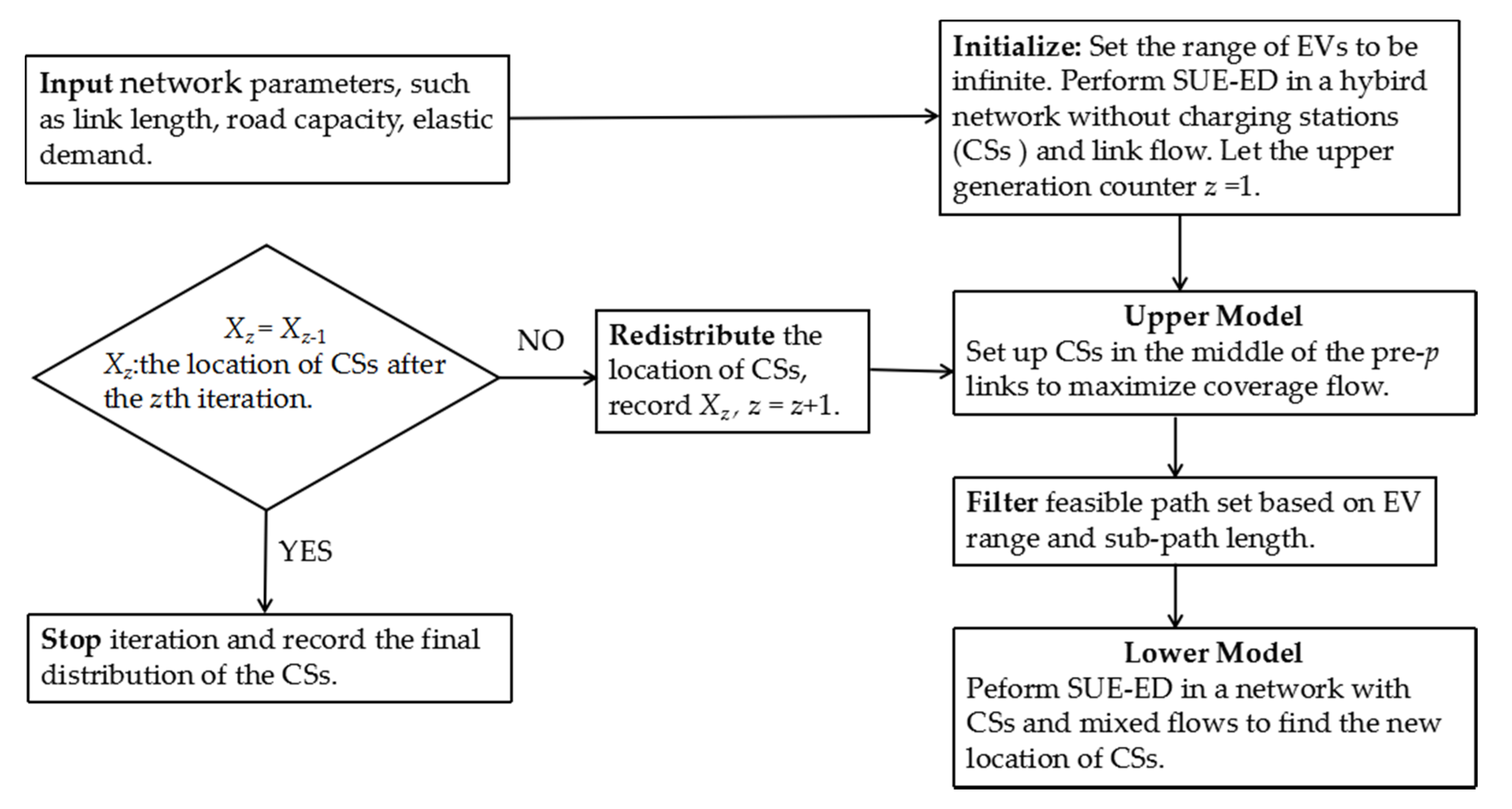
Figure 3.
Nguyen–Dupuis network.

Figure 4.
The flow demands of origin-destination (OD) pair (1,3).

Figure 5.
The sensitivity analysis of the range limit.
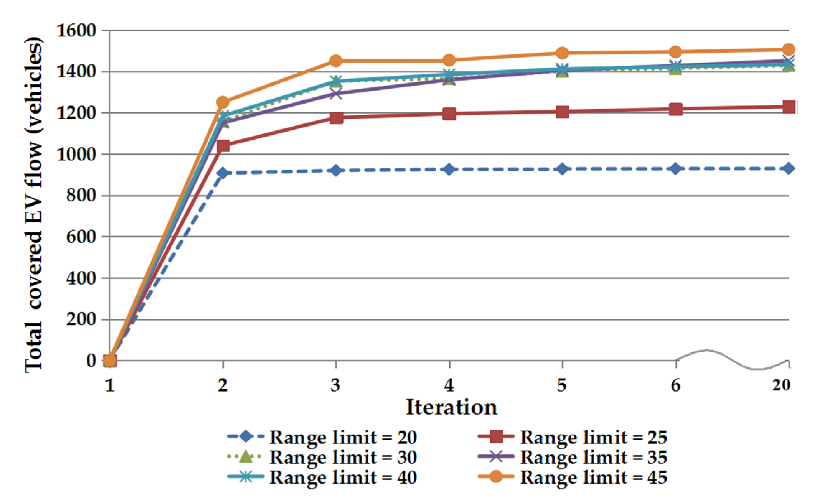
Figure 6.
The sensitivity analysis of charging speed.

Figure 7.
The sensitivity analysis of charging facilities’ utility.

Figure 8.
The sensitivity analysis of waiting cost coefficient K.


Table 1.
Three travel paths of electric vehicles (EVs).
| Scenarios | Conditions | Travel Cost |
|---|---|---|
| 1. A path that can be completed without charging | ≤ | |
| 2. A path that cannot be completed after charging | ≥ or or | |
| 3. A path that can be completed after charging | and ≤ and ≤ and ≤ | + + (K − 1)U |
Table 2.
Path compositions and lengths in the Nguyen–Dupuis network.
| OD Pair | Path Number | Path Composition | Length |
|---|---|---|---|
| (1,2) | 1 | 1-5-6-7-8-2 | 29 |
| 2 | 1-12-8-2 | 32 | |
| 3 | 1-5-6-7-11-12 | 33 | |
| 4 | 1-12-6-7-8-2 | 35 | |
| 5 | 1-5-6-10-11-2 | 38 | |
| 6 | 1-12-6-7-11-2 | 39 | |
| 7 | 1-5-9-10-11-2 | 41 | |
| 8 | 1-12-6-10-11-2 | 44 | |
| (1.3) | 9 | 1-5-6-7-11-3 | 32 |
| 10 | 1-5-9-13-3 | 36 | |
| 11 | 1-5-6-10-11-3 | 37 | |
| 12 | 1-12-6-7-11-3 | 38 | |
| 13 | 1-5-9-10-11-3 | 40 | |
| 14 | 1-12-6-10-11-3 | 43 | |
| (4,2) | 15 | 4-5-6-7-8-2 | 31 |
| 16 | 4-5-6-7-11-2 | 35 | |
| 17 | 4-9-10-11-2 | 37 | |
| 18 | 4-5-6-10-11-2 | 40 | |
| 19 | 4-5-9-10-11-2 | 43 | |
| (4,3) | 20 | 4-9-13-3 | 32 |
| 21 | 4-5-6-7-11-3 | 34 | |
| 22 | 4-9-10-11-3 | 36 | |
| 23 | 4-5-9-13-3 | 38 | |
| 24 | 4-5-6-10-11-3 | 39 | |
| 25 | 4-5-9-10-11-3 | 42 |
Table 3.
The charging facility locations and Electric Vehicle (EV) flows
| Link Node | 1 | 2 | 3 | 4 | 20 | ||||
|---|---|---|---|---|---|---|---|---|---|
| Location | EV Flow | Location | EV Flow | Location | EV Flow | Location | EV Flow | Location | |
| (1,5) | × | 367.5 | × | 219.3 | √ | 197.4 | × | 172.5 | × |
| (4,5) | × | 364.9 | × | 195.4 | × | 172 | × | 143.7 | × |
| (4,9) | × | 164.5 | × | 54.8 | × | 27.4 | × | 0 | × |
| (5,6) | × | 538.5 | √ | 350.1 | √ | 337.1 | √ | 316.2 | √ |
| (5,9) | × | 193.9 | × | 64.6 | × | 32.3 | × | 0 | × |
| (6,7) | × | 499.7 | √ | 337.3 | √ | 363.7 | √ | 380 | √ |
| (7,8) | × | 196.7 | × | 180.5 | × | 210.3 | × | 233.2 | × |
| (8,2) | × | 248.7 | × | 197.8 | × | 219 | √ | 233.2 | √ |
| (1,12) | × | 196.7 | × | 100.5 | × | 83.2 | × | 63.8 | × |
| (11,3) | × | 380.1 | × | 200.4 | × | 175.2 | × | 146.8 | × |
| (12,6) | × | 144.8 | × | 83.2 | × | 74.6 | × | 63.8 | × |
| (12,8) | × | 51.9 | × | 17.3 | × | 8.7 | × | 0 | × |
| (13,3) | × | 157.1 | × | 52.4 | × | 26.2 | × | 0 | × |
| (6,10) | × | 183.7 | × | 95.9 | × | 48 | × | 0 | × |
| (7,11) | × | 302.9 | × | 156.8 | × | 153.4 | × | 146.8 | × |
| (9,10) | × | 201.4 | × | 67.1 | × | 33.6 | × | 0 | × |
| (9,13) | × | 157.1 | × | 52.4 | × | 26.2 | × | 0 | × |
| (10,11) | × | 385.1 | √ | 163 | × | 81.5 | × | 0 | × |
| (11,2) | × | 308 | × | 119.5 | × | 59.7 | × | 0 | × |
Table 4.
The changes in the location of charging stations (CSs) and feasible paths.
| OD Pair | Location 1 | Location 2 | Location 3 |
|---|---|---|---|
| (5,6); (6,7); (10,11) | (5,6); (6,7); (1,5) | (5,6); (6,7); (8,2) | |
| (1,2) | Three paths, including 1,4,5 | Two paths, including 1,4 | Two paths, including 1,4 |
| (1,3) | Three paths, including 9,11,12 | Two paths, including 9,12 | Two paths, including 9,12 |
| (4,2) | Two paths, including 15,18 | One path, 15 | One path, 15 |
| (4,3) | Two paths, including 21, 24 | One path, 21 | One path, 21 |
© 2020 by the authors. Licensee MDPI, Basel, Switzerland. This article is an open access article distributed under the terms and conditions of the Creative Commons Attribution (CC BY) license (http://creativecommons.org/licenses/by/4.0/).
Share and Cite
MDPI and ACS Style
Gao, H.; Liu, K.; Peng, X.; Li, C. Optimal Location of Fast Charging Stations for Mixed Traffic of Electric Vehicles and Gasoline Vehicles Subject to Elastic Demands. Energies 2020, 13, 1964. https://doi.org/10.3390/en13081964
AMA Style
Gao H, Liu K, Peng X, Li C. Optimal Location of Fast Charging Stations for Mixed Traffic of Electric Vehicles and Gasoline Vehicles Subject to Elastic Demands. Energies. 2020; 13(8):1964. https://doi.org/10.3390/en13081964
Chicago/Turabian StyleGao, Hong, Kai Liu, Xinchao Peng, and Cheng Li. 2020. "Optimal Location of Fast Charging Stations for Mixed Traffic of Electric Vehicles and Gasoline Vehicles Subject to Elastic Demands" Energies 13, no. 8: 1964. https://doi.org/10.3390/en13081964
Note that from the first issue of 2016, this journal uses article numbers instead of page numbers. See further details here.