Comparative Study of Powertrain Hybridization for Heavy-Duty Vehicles Equipped with Diesel and Gas Engines

National Research Center “NAMI”, 125438 Moscow, Russia
*
Author to whom correspondence should be addressed.
Energies 2020, 13(8), 2072; https://doi.org/10.3390/en13082072
Submission received: 3 April 2020
/
Revised: 10 April 2020
/
Accepted: 13 April 2020
/
Published: 21 April 2020
(This article belongs to the Special Issue Electric Systems for Transportation)
Abstract
:This article describes a study that aimed to estimate the fuel-saving potential possessed by the hybridization of conventional powertrains intended for heavy-duty vehicles based on diesel and natural gas fueled engines. The tools used for this analysis constitute mathematical models of vehicle dynamics and the powertrain, including its components, i.e., the engine, electric drive, transmission, and energy storage system (ESS). The model of the latter, accompanied by experimental data, allowed for an analysis of employing a supercapacitor regarding the selection of its energy content and the interface between the traction electric drive and the ESS (in light of the wide voltage operating range of supercapacitors). The results revealed the influence of these factors on both the supercapacitor efficiency (during its operation within a powertrain) and the vehicle fuel economy. After implementation of the optimized ESS design within the experimentally validated vehicle model, simulations were conducted in several driving cycles. The results allowed us to compare the fuel economy provided by the hybridization for diesel and gas powertrains in different driving conditions, with different vehicle masses, taking into account the onboard auxiliary power consumption.
1. Introduction
Engines fueled with natural gas are considered possible alternatives to diesel engines when used in heavy-duty (HD) vehicles. Diesel engines, although efficient, have complicated issues regarding exhaust emissions, which compel developers to resort to rather sophisticated solutions to conform with regularly tightened emission requirements. Two components of exhaust gases may be highlighted as problematic, namely the nitrogen oxides and the particulate matter. To reduce the emissions of the former component to the level required by the present-day legislation, a selective catalytic reduction system should be employed, which involves a complex chemical reactor with a closed-loop control system and an onboard storage for the additional chemical agent (ammonia) [1]. Reducing the particulate matter requires using filters, which also constitute complex systems that involve an electronic control that regulates the process of regeneration [1]. It should also be noted that diesel engine operating regimes having minima of the two mentioned exhaust components generally do not coincide, which complicates the engine calibration [1]. In contrast, gas-fueled engines have drastically lower raw emissions of particulate matter [2,3,4] and can operate with the stoichiometric air-to-fuel ratio [5,6], which makes it possible to reduce emissions using less complex three-way catalytic converters [5] that provide more efficient abatement at lower costs. Fuel costs are generally considerably lower for gas (although this is not included in the scope of this work, which is only dedicated to the technical issues). The complicating aspect of replacing diesel engines with gas engines is the necessity of having an onboard storage for the compressed or liquefied gas, which constitutes a complex system that has its own cost, service, safety, and other issues. Therefore, whether to choose a gas-based vehicle or stay conservative with a diesel-based option becomes a trade-off decision.
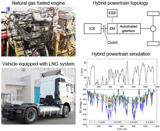
During the past few years, the National Research Center “NAMI” has been conducting an R&D project in cooperation with one of the country’s major producers of heavy-duty vehicles. The project was aimed toward developing a gas-fueled engine family derived from the diesel engine that was newly developed by the aforementioned HD vehicle manufacturer. One can find the details on the project and its results in References [7,8,9]. The main outcomes of the project were the gas-fueled engines (see example in Figure 1) operating with the Otto and Miller thermodynamic cycles. The engines were installed in vehicles intended for long-haul operations (also shown in Figure 1) and tested in road conditions.
The present work aimed to provide further elaboration of powertrains equipped with the developed gas engines, specifically on the prospects of their hybridization. The primary motivation behind this was to compare the fuel economy improvements that can be achieved by the hybridization of a diesel-based powertrain and a gas-based powertrain. It is assumed that such a powertrain modification could be relevant for those HD vehicles, whose operating schedules include a considerable share of city and suburban haulage since the major effect of HD powertrain hybridization is expected in conditions allowing for intensive use of regenerative braking, which is the most efficient tool for increasing the fuel economy of vehicles with large masses [10].The published studies (see, for example, [11,12,13,14]) have demonstrated that hybrid HD vehicles having a gross mass ranging 16 to 36 tons possess a significant fuel-saving potential in city driving conditions, especially in the case of full hybridization, which offers up to 35% fuel consumption reduction. The mild degree of hybridization is able to provide moderate fuel savings of about 10%.
The fuel economy of powertrains, which use different kinds of fuels, cannot be compared directly. One can evaluate the energy content of the consumed fuel [15], or the CO2 emissions of compared vehicles [12,15], or the economic aspect, i.e., fuel price [12,15,16]. This work employed another approach stemming from the goal of hybridization, namely to reduce the fuel consumption relative to the baseline powertrain. This allows for comparing the percentages of vehicle fuel economy obtained for each considered powertrain rather than the absolute values of fuel consumption. The study was conducted by means of simulations based on mathematical models validated using experimental data.
The layout of the article has the following structure. The next section (Section 2) substantiates the choice of the hybrid powertrain design to be considered in the study. Section 3 describes the mathematical models of the vehicle and the powertrain components. It is followed by a section (Section 4) overviewing the control strategy implemented within the hybrid powertrain model. The driving cycles employed in the simulations are presented in Section 5. The models of conventional vehicles equipped with all the considered engines are validated in Section 6. The model analysis of the powertrain hybridization is presented in Section 7. Finally, Section 8 contains conclusions drawn from the conducted study and outlines further research.
2. Hybrid Powertrain Design
2.1. Selection of the Hybrid Powertrain Topology
Internal combustion engines (ICEs) intended for HD vehicles are remarkably efficient in a wide range of operating modes. Brake-specific fuel consumption (BSFC) becomes significantly higher only at small loads, which, in a hybrid electric vehicle (HEV), may be avoided by electric driving or, in the case of insufficient battery energy, by additional loading of the ICE. The concept of the optimal operating line (OOL), i.e., the locus of operating points having a minimum BSFC for a given power, is undoubtedly efficient in light duty applications where ICEs have a significant BSFC gradient; however, in the case of HD engines, the OOL is not as clear. In the first place, it requires employing a continuously variable transmission (CVT), which in the case of HD vehicles, can be either electric (corresponding to a series HEV topology) or electromechanical (the power-split topology). Both options (frequently called e-CVTs [17]) imply using two electric machines, which complicates the transmission and makes it more expensive. Generally, e-CVTs have a lower efficiency than stepped mechanical transmissions, and using them only makes sense if OOL tracking provides an increase of the ICE efficiency, which is significantly higher than the effect of impairing the efficiency using an e-CVT. In the case of an HD engine, OOL tracking may increase its efficiency only slightly, and considering a relatively low e-CVT efficiency, the overall fuel-saving effect will most likely be small or, in some cases, even negative [13]. This, together with the first aspect (complex and expensive transmission), makes e-CVT-based topologies hardly affordable, especially when it comes to issues of producing and owning such vehicles.
The parallel topology (Figure 2) can be derived from a conventional transmission (with an automated stepped gearbox) through moderate design changes. It implies placing an electric machine (EM) between the ICE shaft and the gearbox input shaft. It is advisable to place the automated clutch between the ICE and the EM to disconnect the former from the transmission and therefore allow the vehicle to be driven solely by the electric machine. The energy storage system (ESS) is connected to the traction electric drive using a DC link shown by the dotted line in Figure 2. The direct mechanical connection established between the ICE and the EM when the clutch is locked allows for the efficient transmission of power from the ICE to the ESS when it is necessary to replenish the latter or to load the former to avoid non-efficient operating regimes.
Placing the EM before the gearbox allows for providing a considerable range of electric driving (in terms of both speed and tractive force) without oversizing of the electric machine, which usually takes place in the topologies where the EM is connected to the driving wheels through a reduction gear that has a constant speed ratio. On the other hand, losses in the gearbox reduce the efficiency of the transmitting power from the EM to the driving wheels and backwards (regenerative braking).
2.2. Selection of the Powertrain Components
While the set of internal combustion engines to be employed in the studied powertrains was defined (i.e., the diesel and two gas engines), the electrical components were to be selected or designed. Considering the available technical resources and the objectives of the study, units available “from the shelf” were preferred over theoretical ones. In particular, the prototype traction electric drive was acquired from one of the commercially available hybrid units intended for HD vehicles. When used in an HEV with the gross weight considered in this work (35–44 tons), the power and torque characteristics of the electric drive (see Section 3.4 for details) correspond to an intermediate solution between the full and mild hybrids.
Two options for the engine control at vehicle stops were considered, namely idling and switching the engine off and starting it back when the vehicle resumes moving (i.e., the start–stop feature). The latter option was assumed to be implemented using an “enhanced” starter rather than the traction electric drive to prevent impairing the vehicle dynamics.
The energy storage system (ESS) is one of the key components in a hybrid powertrain, which defines the amount of regenerated braking energy and the vehicle performance in the pure electric driving mode. The prevailing ESS technology in the field of hybrid and pure electric vehicles are accumulator cells, which are lithium-ion for the most part [19]. Their specific energy capacity and power, which have noticeably increased over the years [20])], along with their moderate prices make them well-suited for passenger and light-duty commercial vehicles. Their known vulnerability to high and low temperatures (capacity and efficiency drop, accelerated degrading) can be alleviated using appropriate temperature management [19], at least in hybrid vehicles, where engine heat can be utilized for that purpose. The cycle life of typical lithium-ion cells, although relatively short (a typical value is around 3000 cycles, but may be lower), is nevertheless admissible for electric vehicles since they employ large battery packs that allow for traveling up to a few hundred kilometers per charge–discharge cycle. Hybrid vehicles, especially non-plugin vehicles, have significantly smaller batteries, which compels developers and producers to resort to more advanced (and expensive) accumulator cells that have higher power densities and longer cycle lives.
When it comes to the hybridization of heavy-duty vehicles, the following specifics of long-haul vehicle applications have to be taken into account while selecting the ESS type. Due to the large mass of such vehicles, the ESS should be able to deliver and consume high amounts of power (over 100 kW) continuously. An HD vehicle usually has a long service life and is operated intensively (on an everyday basis), which entails a large mileage from hundreds of thousands to even millions of kilometers. Throughout the service period, the number of overhauls should be minimal. The replacement of powertrain components, especially expensive ones, is undesirable (the operating life of the powertrain and its major components is to be equal to that of the vehicle). Additional expenses brought about by introducing advanced powertrain technologies should be (at least) compensated for by the economic effect provided by those technologies (e.g., reduced fuel consumption). Climatic operating conditions of the heavy-duty vehicle fleet vary greatly, including both extremely cold and warm regions.
To provide a longer cycle life of accumulator-based solutions, one should use “shallow” charge–discharge cycles. Together with the requirement for higher power, this implies that large batteries are to be used in HD vehicles. As a result, even for hybrid applications, which offer a relatively small pure electric driving range, the battery tends to be oversized due to the necessity in meeting both the power and cycle life requirements.
A known alternative for high-power ESSs are supercapacitors (SCs), which the literature claims as a promising technology for heavy-duty vehicles [11,21,22,23,24]. One has to admit that the characteristics of supercapacitors include both substantial advantages and adversities. Among the former, one can provide high operating currents and, consequently, a high power density [25,26]. A single SC cell having a nominal voltage of 3 V can operate continuously with currents up to 300 A and, for a limited time, over 1000 A. The cycle life of supercapacitors is outstandingly higher than that of lithium-ion accumulators and exceeds 1 million cycles [25,26]. Additionally, supercapacitors have a wide operating range of low temperatures, which can reach −40 °C. For example, when used in engine-cranking applications, an SC can start an engine smoothly in a −25 °C ambient temperature [26]. Thus, supercapacitors do not impose the same strict requirements regarding the low-temperature management as accumulators do. On the other hand, the following shortcomings of supercapacitors should be taken into account. Their energy density is far lower (about 95% lower on average) than that of lithium accumulators. The prices for a kWh of supercapacitors are at least 20 times higher than those of the typical lithium cells. For advanced, high-power, long-life accumulators used in compact batteries of hybrid vehicles, this price ratio may be smaller, although not drastically. Like lithium-ion accumulators, supercapacitors are vulnerable to high-temperature degradation; therefore, they require effective cooling systems [25]. Yet another feature may be counted as both positive and negative, namely the proportionality between the supercapacitor voltage and its state of energy. On the one hand, this allows an ESS management system to determine the state of energy using simple voltage monitoring. In contrast, lithium-ion accumulators, especially the LiFePO4-type accumulators, require battery management systems to have sophisticated algorithms for the indirect determination of the state of charge [27] due to its substantial independence from the accumulator voltage. On the other hand, the said proportionality results in a wide operating range of the supercapacitor voltage is much wider than that of lithium-ion accumulators, which raises the question of matching this range with the operating voltage of the traction electric drive. One known solution is employing a DC–DC converter that keeps the input voltage of the electric drive at a reference level, while the supercapacitor voltage travels through its operating range [24,28,29]. This ensures that the traction drive will be able to deliver its rated power independently (to a certain extent) of the ESS voltage. The complication of this approach is, obviously, the need for a high-power buck–boost converter, which entails additional costs, weight, occupied space, and finally, yet importantly, power losses due to voltage transformation. One can expect a 95% peak efficiency at most from such a converter, which is rather noticeable for the powertrain energy balance considering that the major power flow will be transmitted through this converter. Another solution is a direct DC connection between the supercapacitor and the traction drive inverter [29]. This makes the operating characteristics of the drive variable and needs to be addressed in the control algorithm of the powertrain. In the described study, both solutions were compared in terms of the resulting fuel economy and ESS efficiency.
For commercial vehicles, all the mentioned virtues of supercapacitors—high power, long cycle life, and wide operating temperature span—are particularly advantageous. When considering the drawback of low energy density, one can conclude that unlike for pure electric vehicles, for non-plugin hybrids, this is not a critical issue, although the large weight of HD vehicles, of course, does require a proportional energy content of the ESS that can recuperate the bulk of the braking energy. The supercapacitor cost, however, is an issue that raises concerns regarding the additional expenses entailed by hybridization. Since the amount of regenerated energy that can be stored within the ESS is the decisive factor of fuel economy (in the case of HD vehicles), the ESS capacity is a result of a trade-off between lower fuel expenses and higher ESS costs. Therefore, establishing the influence of the ESS energy content on the fuel economy becomes an additional objective of the study.
The prototype of the supercapacitor-based ESS used for this study has been taken from the powertrain of a hybrid city bus that belonged to a limited series produced earlier. The ESS in that bus has an electric capacitance of 28 F and a maximum voltage of 650 V, providing an energy content of 1.6 kWh. The maximum continuous current is 300 A for both discharging and charging. Considering the voltage operating range of 300–640 V, the maximum power delivered by the SC amounts to 90–195 kW. To obtain the characteristics of the prototype supercapacitor, several field experiments were conducted involving the mentioned hybrid bus. During those tests, the supercapacitor current and voltage were being measured and logged while the bus was being driven through predetermined velocity patterns.
3. Mathematical Models
3.1. Vehicle Dynamics
Simulations aimed at the calculation of the fuel economy and assessment of the powertrain operation usually replicate vehicles moving through driving cycles that model real-world driving conditions. Cycle schedules do not include the driving trajectory, and, thus, when modeling, the vehicle motion is considered linear. Furthermore, there were additional assumptions that were made in this work to derive the vehicle dynamics model. The tire slip is neglected due to the assumption that the maximum adhesion coefficient is high, and thus, a sufficient tractive force is exerted with a small slip. The model also neglects the dynamics of wheel vertical forces and variations of the wheel radii. Given these assumptions, the model of the vehicle linear motion can be presented as the dynamics of a single lumped mass:
where is the vehicle velocity; is the vehicle mass; is the torque at the driving wheels; is the wheel radius; is the wheel inertia; n is the number of wheels on the vehicle (including the trailer’s wheels); and , , and are the resistance forces.
The rolling resistance force is calculated using the following formula: , where is the acceleration due to gravity and is the dimensionless coefficient of tire-rolling resistance. When identifying the model parameters from the coast-down test results, it was found that the function was satisfactorily approximated using the known quadratic expression: [30], where is the rolling resistance coefficient at near-zero velocity and is the factor of the velocity-dependent growth of the rolling resistance. The rolling resistance force calculated with these formulae was assumed to be equal (i.e., averaged) for all the tires of the vehicle.
A well-known empirical formula is used for calculating the aerodynamic resistance force:
where is the air drag coefficient of the vehicle, is the vehicle frontal area, and is the air density.
The grade resistance force is a projection of the vehicle gravity force vector onto the road plane, which is calculated as follows: , where is the road inclination angle (positive for an ascending slope).
3.2. Internal Combustion Engines
The powertrain model elaborated in this work used the quasi-static approach for the simulation of the internal combustion engines. The engine characteristics were obtained experimentally in steady operating regimes and then implemented in the form of lookup tables. During simulations, the characteristics were interpolated using dynamic values of the engine rpm and the torque command calculated using the model. The required characteristics of the engines were obtained via laboratory dynamometer tests. In those tests, several parameters were measured and logged, namely the shaft speed, shaft torque, and fuel consumption, which were then employed for modeling purposes.
Figure 3 shows the BSFC map of the diesel engine and its maximum torque curve denoted as “Max. trq.” The main performance parameters of this engine confirmed using the tests were as follows: rated power 331 kW (at 1900 rpm) and 1985 Nm maximum torque (at 1300 rpm).
Similar maps were built from the dynamometer test data for the gas engines (Figure 4). The main performance parameters of these engines were also confirmed: gas Otto’s cycle—rated power 326 kW (1900 rpm), maximum torque 1900 Nm (1300 rpm); gas Miller’s cycle—rated power 384 kW (1900 rpm), maximum torque 1950 Nm (1400 rpm).
One can notice that the engine with the Otto’s cycle has a steeper gradient for the BSFC than that of the Miller-cycle engine, especially at low loads. This suggests that a wider part of the engine map should be excluded (if possible) from operating regimes through hybridization in the case of the Otto engine. It can also be seen that the Miller-cycle engine has an apparent torque dip at low shaft angular speeds, which should be compensated for using the additional torque of the electric machine (i.e., the “torque boost” feature).
3.3. Transmission
The transmission model was derived under the assumption that all its shafts were rigid (i.e., shaft torsional stiffness was neglected). Both the conventional stepped transmission and the transmission of the parallel hybrid topology have three operating regimes defined by the automated clutch state: whether it is disengaged, slipping, or engaged. In the first and the second states, the ICE shaft has a separate degree of freedom, which, for the hybrid transmission, yields the following system of equations:
where and are the shaft speeds of the ICE and electric machine, respectively; and are the shaft torques of the ICE and electric machine, respectively; is the clutch torque; and are the inertias of the ICE and electric machine, respectively; and are the ratios of the gearbox and final drive, respectively; and and are the efficiencies of the gearbox and final drive, respectively. The efficiencies are raised to the power of the torque sign function in order to take into account both traction and braking torques entering the transmission.
The term introduces a relation between the direction of the clutch torque and the speed differential of the input and output parts of the clutch. When the clutch becomes fully engaged, the separate equation of the ICE shaft dynamics, as well as the torque , can be excluded from the transmission model, thus eliminating one degree of freedom.
To derive the model of the conventional transmission from the system (Equation (3)), one should exclude the terms associated with the electric machine and replace the angular speed with that of the gearbox input shaft.
3.4. Electric Drive
The electric drive, just like the internal combustion engines, was modeled using experimental static maps. Laboratory tests allowed for obtaining the torque and efficiency characteristics of the traction electric drive (electric machine + inverter) for two voltage levels, namely 650 V and 450 V, which covered the bulk of the prototype supercapacitor operating range. Between these voltages, the characteristics were interpolated, and were extrapolated below 450 V. The main parameters of the electric drive obtained from the experimental data are summarized in Table 1.
Figure 5 shows the efficiency map and the maximum torque characteristics of the electric drive in motor mode.
Given the electric machine torque (commanded by the control system) and the shaft speed (calculated by the transmission model), as well as the supercapacitor voltage calculated via its model, one can obtain the electric drive current at the DC side:
where is the electric drive efficiency, taking into account the torque direction (positive for the motor mode). The current calculated with this formula is used by the SC model as the input signal.
3.5. Energy Storage System
The following considerations were taken into account when choosing the approach to mathematical modeling of the supercapacitor. Chemical processes within the SC lie beyond the scope of the research. At the current stage, temperature effects are also neglected under the assumption that the powertrain operates within a moderate range of temperatures, which imposes no substantial effect upon the supercapacitor characteristics. The operating parameters of the SC relevant for the powertrain modeling in this study were the current, voltage, efficiency, and energy content. These considerations suggest using equivalent circuit modeling, which is a widely employed approach for the analysis of ESS not as electrochemical systems but rather electrical components of the powertrain. References [25,31,32] describe an equivalent circuit for the supercapacitor in the form of a “ladder” with each “step” consisting of a capacitor and a resistance. Depending on the required model fidelity, one can use different numbers of “steps,” which in the simplest case, would be a single one. The comparison performed in this work with the involvement of experimental data has shown that a reasonable trade-off between model accuracy and complexity is provided by a circuit consisting of three “steps,” as shown in Figure 6.
In this scheme, , , and are the internal resistances; ,, and are the capacitances; and and are the voltage and current at the supercapacitor electric terminals.
From the equivalent circuit, one can derive the following equation system using Kirchhoff’s current and voltage laws:
where , , and are the voltages within the sub-circuits corresponding to each “step” of the “ladder.”
The initial conditions can be obtained for this model from the assumption of equality between the voltages of all the capacitors, which takes place when no load is applied and transient processes have ended: . Substituting this condition into the first equation of the system (Equation (5)) yields the initial condition for the integral term:
The term is the total capacitance of the “ladder.” Identification of the model parameters using experimental data showed that the best accuracy for voltage calculation was obtained when the sum was equal to the rated capacitance of the modeled SC. Furthermore, this provided a correct calculation of the supercapacitor energy content with no need for ad hoc corrections.
Figure 7 shows the results of modeling that simulated two experiments involving the supercapacitor installed within the powertrain of the hybrid city bus mentioned in Section 2. The bus was driven in the pure electric mode through velocity patterns consisting of accelerations and decelerations. The top plots demonstrate the supercapacitor current logged during the experiments (positive for charging). The current was used as the input signal for the equivalent circuit model, which responded with the calculated voltage. The latter is shown in the bottom plots (denoted as “Model”) along with the measured voltage (“Experiment”). The identification of the model parameters was performed using the criterion of the minimum root mean square error (RMSE) of voltage calculation. The parameter set satisfying this criterion is listed in Table 2. The RMSEs obtained with these parameters amounted 0.7–3% in about a dozen experiments.
The equivalent circuit includes the internal resistances, which not only provide a voltage drop, but also introduce the dissipation of energy, and therefore, allow for calculating the capacitor efficiency. To do this, it is necessary to determine the power dissipated at the resistances.
The current through the resistance is equal to that at the SC terminals, i.e., . While deriving the system (Equation (5)), one can find that the current through the second resistance is equal to . The current in the third “step” is equal to . Therefore, the total power loss is:
The supercapacitor net power . The total power drawn from the SC or received by it is a sum of the net power and the loss power, taking into account the signs thereof. These considerations result in the following expression for the SC efficiency:
Note that is positive for charging.
Figure 8 demonstrates the simulation results for yet another one of the mentioned field tests, in which the supercapacitor was discharged with the maximum continuous current and then charged back to the initial voltage. Three upper plots show the voltage, current, and net power of the SC, respectively. The fourth plot demonstrates the components of power dissipation associated with the three internal resistances of the equivalent circuit. One can see the clear differences in the dynamics of these components. The first term is the major contributor to the power dissipation. The dynamics of this term is defined by the dynamics of supercapacitor loading (i.e., dynamics of the current). The second and third terms constitute processes with slower dynamics and lower amplitudes. The SC efficiency (the bottom plot) diminished along with the voltage, while the loading current remained constant, as well as the power dissipation at the resistance . However, the power losses at the two other resistances grew due to dynamics of the currents at the capacitors and . Analysis of the obtained results suggests that when using the considered supercapacitor as the ESS in a hybrid powertrain, one should avoid a deep discharge (i.e., below 450 V), either using the control strategy or via supercapacitor sizing or, most likely, both.
It is worth noticing the interval of transition between discharging and charging (in the vicinity of the 14th second), where the power dissipation at drops down to zero while the powers at and continue to attenuate at the rates defined by the parameters of the corresponding “steps” of the equivalent circuit. After the load removal, the capacitors , , and exchange energy between each other until their voltages become equal. This process is accompanied by the dissipation of energy at the resistances and . If no external load is present during these periods of voltage stabilization, the efficiency of the SC becomes negative. However, in the estimation of the SC mean efficiency, such energy losses may be assigned to the preceding operating interval, which allows for avoiding an unnecessary introduction of the negative efficiency.
An alternative way of determining the supercapacitor efficiency (the average for a certain operating period) stems from the fact that the equivalent circuit model incorporates the power dissipation, and the supercapacitor voltage calculated by it reflects the actual state of energy (at least under no-load conditions). Therefore, one can integrate the net power and multiply it by the average efficiency, which is calculated to bring the integrated energy level to that of the equivalent circuit model by the end of the operating cycle. This can be expressed as the following equation:
where is the average efficiency of the SC during the given period, is the end time of the period, and is the SC voltage at the end of the period.
3.6. Onboard Power Consumers
The main onboard power consumers of an HD vehicle are the air brake compressor, power steering, air conditioner compressor, engine oil and coolant pumps, engine fan, and electrical accessories. In a conventional powertrain, most of these are powered mechanically by drives connected to the engine shaft. Those of them not having disconnecting mechanisms, consume some power even in the idle state. In the literature [13,33], one can find typical ranges of the consumed power for each of these components as a function of the engine shaft speed as well as their operating cycles based on the recommendations of the SAE J1343 standard [34]. An operating cycle is defined by two numbers, namely being the averaged period of the operating cycle and being the fraction (i.e., percentage) of the operating cycle when the component is engaged. Table 3, based on the information from References [13,33], summarizes the power and duty cycle data for the auxiliaries included in the model of the conventional powertrain. In this table, “A/C” stands for the air conditioning and “Electrical acc.” denotes the low-voltage electrical accessories. The columns “Min. power” and “Max. power” contain the ranges of power consumption corresponding to the engine rpm range, which was from 500 rpm (the lower power value) to 2000 rpm (the higher power value).
The power feeding the electrical accessories is drawn from the engine shaft through the alternator, whose efficiency, obtained from the known literature [35,36], was taken into account in the elaborated model.
The engine coolant and oil pumps are not listed in Table 3 since in this work, they were considered as parts of the engine system. Their power demand is taken into account by the fuel consumption characteristics of the engines since the latter underwent the bench tests with the said auxiliaries installed. The coolant and oil pumps were also considered identical for both the conventional and the hybrid powertrains.
In a hybrid powertrain, the electrified auxiliary components are regulated independently from the engine operating regime, therefore consuming the exact amount of power required for their operation [13]. Table 4, based on the information from [13], shows the average power and operating cycle data for the auxiliaries assumed to be electrified in the hybrid powertrain. Besides the conventional auxiliaries, the cooling system of the high voltage components was taken into account (denoted as HV cooling).
A DC–DC converter was considered as the interface between the low voltage auxiliary system and the high voltage traction system.
4. Hybrid Powertrain’s Control Strategy
This section gives a brief overview of the control strategy developed for the hybrid powertrain model, highlighting its essential structure and operating principles.
If the modeled HEV is equipped with the start–stop feature, the control algorithm of the latter is quite simple: when the vehicle stops, the engine shuts down; the engine starts again when the vehicle resumes moving (i.e., velocity crosses the minimum threshold). When the ICE is on, the powertrain can operate in one of the two basic modes, namely the electric mode or the hybrid mode, which is illustrated in Figure 9. The former implies for the ICE to be in the idling state having the corresponding torque , while the electric machine drives and decelerates the vehicle; the EM torque is a function of the accelerator (acc.) and brake pedal signals. In the hybrid mode, both the ICE torque and the electric machine torque are functions of the accelerator and brake signals, as well as the supercapacitor current and voltage .
In Figure 9, several conditions (C1–C6) are assigned to the transition arrows, as well as the logical relations between these conditions (i.e., “and” and “or” operators). The conditions are detailed in Table 5.
The parameters , , , and specify the upper and lower thresholds for the vehicle velocity and accelerator signals. The default values of and are 25 km/h and 15 km/h, respectively. The default values of and correspond to 50% and 10% of the maximum ICE torque. These values are used when the ESS voltage stays near its maximum (650 V). When the voltage lowers, the thresholds decrease to engage the ICE earlier and to reduce the electric machine traction torque, preventing an excessive consumption of the supercapacitor energy.
Besides the electric mode, the engine becomes disconnected from the transmission upon gear shifting. During a shift, the electric machine provides gear synchronization.
The hybrid mode implies the torques of the ICE and the electric machine should be combined. When the SC voltage drops below the lower threshold (the default value is in the range of 500–550 V), the ICE begins delivering an excessive power consumed by the electric machine whose torque becomes a function of the SC voltage drop (the deeper the discharge, the higher the torque). When the driver’s torque request exceeds the maximum ICE torque, the electric machine provides the “torque boost” in accordance with the map shown in Figure 10 using the example of the diesel-based powertrain (the resulting curve of the hybrid unit’s maximum torque is denoted “Hybrid max. trq”). Like the thresholds of the velocity and accelerator signals, the boosting torque constitutes a function of the ESS voltage.
5. Driving Cycles
Several driving cycles intended for heavy-duty vehicles were employed in the simulations to represent the variety of possible driving conditions. These included urban and suburban cycles, which constitute the major interest of the study, as well as highway cycles.
The driving cycles employed in the simulations are shown in Figure 11. The GOST cycles are road-performed (rather than using a chassis-dynamometer) schedules provided by a national standard named the GOST. All the driving cycles, except for the WHVC, imply level roads.
6. Validation of the Conventional Vehicle Model
In the R&D project mentioned in the introduction, several road tests were conducted in the GOST driving cycles involving vehicles equipped with the developed diesel and gas engines. Furthermore, by way of comparison, a vehicle equipped with a production gas-fueled engine was tested in the same driving conditions. The logged parameters were the vehicle velocity, engine rpm, and fuel consumption. The logs allowed for simulating the tests and validating the model of the conventional vehicle.
The baseline vehicle was an articulated road train (tractor-trailer) intended for long haulage. It was equipped with a manual 16-speed mechanical gearbox with two ranges, the high and low, with eight gears each. In normal driving conditions, the former is usually preferred over the latter. The test mass of the vehicle was 44,000 kg (equals to the tractor-trailer gross mass).
Prior to the driving cycle tests, coast-down experiments were performed to estimate the rolling and air resistance forces. Analysis of the coast-down results and the vehicle’s technical specification available from the manufacturer allowed for identifying the parameters of the model of vehicle dynamics (Equation (1)), which are specified in Table 6.
Table 7 shows the fuel economy data obtained using the field experiments and simulations, as well as the simulation errors, for the vehicles equipped with the three mentioned engines.
The higher error for the production gas engine in the city cycle resulted from the unknown experimental velocity data, which compelled to use the velocity log from another vehicle’s test. Despite the same driving schedule, the velocity profiles most likely had certain differences since the accuracy of road-performed cycles strongly depends on the driver’s behavior, which obviously cannot be repeated precisely from test to test.
In general, the model was considered to have sufficient accuracy for performing further simulations with the hybrid vehicles.
7. Model Analysis of the Powertrain Hybridization
Considering the main objective of the study and having analyzed the specifics of the devised hybrid powertrain design, the simulation program was formulated as the following sequence of tasks:
- Estimate two approaches to match the electric drive voltage to that of the supercapacitor, namely by employing a DC–DC converter and directly interfacing the two devices.
- Estimate the powertrain characteristics with different ESS energy contents.
- Having selected the “optimal” solution regarding the ESS energy and the electrical interface, use this solution in comparative simulations estimating the fuel consumption of the conventional and hybrid powertrains. Calculate the fuel economy of the HEVs relative to the conventional vehicles.
- Estimate the influence of the vehicle mass on the relative fuel economy.
The simulations were conducted in identical driving conditions for all the studied powertrains. The compared variants of HEVs shared the same adjustments of the control system with slight variations due to differences in the characteristics of the engines. The gearbox shift map, which was common for both the conventional and the hybrid powertrains, was defined in a way similar to that employed within the Vecto software tool [36].
Figure 12 shows an example of simulation results obtained in the urban part of the WHVC driving cycle for the HEV equipped with the Otto-type gas engine that had the start–stop feature. (“EM” denotes the variables related to the electric machine).
Since the considered hybrid powertrain had no external ESS charge feature, the condition of the energy balance should be pursued in the simulated driving cycles. This means that the ESS energy level at the end of the cycle has to be equal to that observed at the beginning of the cycle. This ensures that no ESS energy is spent without replenishing it and no fuel is consumed to excessively charge the ESS. Originally, since the HEV’s control system was not intended to achieve the precise energy balance within a specified time interval, an ad hoc adjustment was introduced, which gradually “pulled” the ESS state of energy toward the initial value when approaching the end of the driving cycle. With the energy balance condition achieved, the fuel economy of the HEV relative to the conventional vehicle was calculated as follows:
where and are the fuel consumptions (L/100 km or m3/100 km) of the conventional and hybrid vehicles, respectively.
The average auxiliary power consumption was calculated from the simulations of all the employed driving cycles. For the conventional vehicle, it amounted 6–7 kW for the urban and suburban conditions and 2–4 kW for the highway schedules. For the hybrid vehicle, it was lower (due to the engine-independent control), with 3.5–4 kW and 1–2 kW, respectively.
Tasks 1 and 2 formulated at the beginning of the section were solved simultaneously. To do this, two sets of simulations were conducted, one of which implemented the direct connection between the ESS and the electric drive, while the other involved a DC–DC converter as the interface. Each set included simulations with different numbers of supercapacitors, ranging from one (1.6 kWh) to four (6.4 kWh). When employing more than one SC unit, the electrical connection between the units was assumed to be parallel. When modeling the variant with a DC–DC converter, the latter maintained the electric drive input voltage at a constant 640 V. The efficiency of the converter was assumed to be 95% (the actual value would most likely be lower).
Figure 13 demonstrates the ESS voltage time histories calculated for the urban/suburban part of the WHVC driving cycle. From the plots, it is clear that using a larger ESS allows for decreasing both the depth of the discharge and the voltage amplitude. Note that this effect is the most pronounced when adding the second SC unit.
Table 8 summarizes the results of the simulations for the HEV equipped with the Otto-type gas engine and having the start–stop feature. The data were obtained in the WHVC urban/suburban cycle. Other powertrain variants were also estimated and showed similar results.
The results show an evident drawback of employing the DC–DC converter, which is a decrease of the fuel economy effect by 4–5%. The lowest fuel savings were obtained when using one SC unit. Although the DC–DC converter prevents the electric drive power from diminishing, therefore keeping the potential of regenerative braking at the maximum level, the SC is discharged below the threshold of the favorable efficiency. Additional losses are introduced by the DC–DC converter itself. As a result, the positive effect of the maximum electric drive power available throughout the driving cycle is not able to outweigh the adverse effect of the lowered system efficiency. However, the simulations with the higher ESS energy contents show that keeping the SC efficiency at a good level does not eliminate the effect of the diminished fuel economy. Moreover, despite the increased ESS efficiency, the fuel economy difference between the two interface options changes negligibly. This suggests that the critical factor is the power loss within the DC–DC converter rather than in the supercapacitor.
Figure 14 shows the average supercapacitor efficiency and the relative fuel economy of the HEV as a function of the ESS energy content, where the plots have resulted from the driving cycle simulations. The efficiency plot denoted “Equiv. circ.” was derived using Equation (8), while the second plot, “Const. eff.,” was calculated using Equation (9). The difference between the plots stems from the extra-low load regimes where the efficiency of the SC may become negative (see Section 3.5). If those regimes are lumped into the bulk of the power losses, the line “Equiv. circ.” lifts toward the second line, eventually coinciding with it. The effect of adding the third and fourth SC units is not so appreciable, while the cost of an ESS having that size may be rather high, outweighing the fuel savings.
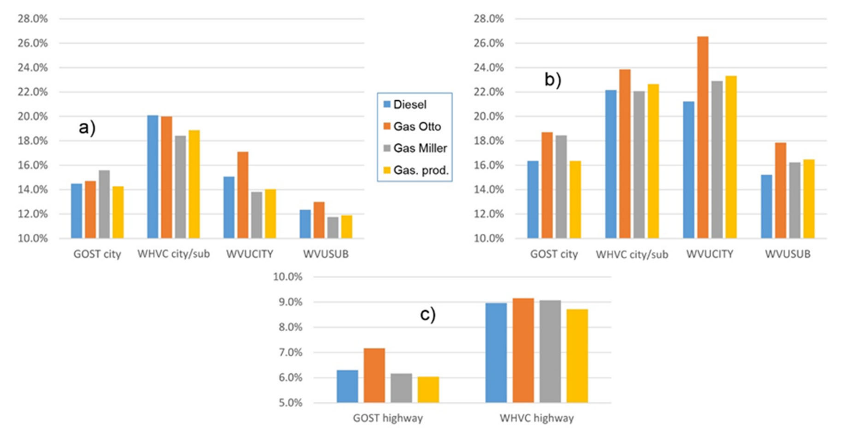
Solving tasks 1 and 2 allowed us to formulate the “optimal” solution regarding the ESS design: it should consist of two SC units having a total energy content of 3.2 kWh and interfacing with the traction electric drive via a direct DC link. This solution was used in the simulations relating to task 3. The results thereof are presented in Figure 15 in the form of histograms showing the relative fuel economy provided by the hybrid powertrains based on all the mentioned ICEs in different driving cycles.
In general, the hybridization provided a similar fuel economy effect for both the diesel-based and gas-based powertrains. The average differences of the relative fuel economy between the gas-based HEVs and the diesel-based HEV are listed in Table 9.
The most pronounced effect of the hybridization is observed with the Otto gas engine. In the conventional powertrain, the Otto-cycle engine is up to 5% less effective than the two other gas engines, while the hybrid powertrain allows this engine to reach the absolute fuel economy values of its counterparts.
The fuel economy effect provided by the hybridization mainly depends on two factors: driving schedule and employing the start–stop feature. The former relates to the characteristic called the kinetic factor [10]. It expresses the share of “acceleration–deceleration” driving that directly determines the intensity of using regenerative braking, which in turn, is the major factor of a heavy-duty HEV’s fuel economy. From the simulation results without the start–stop feature (i.e., when regenerative braking is the decisive factor of the fuel economy), one can conclude that among the used driving cycles, the city/suburban part of the WHVC has the highest kinetic factor.
The effect of introducing the start–stop feature is particularly pronounced for the gas-based HEVs, especially in the driving cycle containing the highest share of stops, namely the WVUCITY cycle. This is due to the ratio of the idle fuel consumption rate to the maximum fuel rate of the gas engines being approximately two-fold that of the diesel. In other words, the gas engines have a larger share of the idle consumption, which makes its elimination an effective measure to increase the fuel economy. In the absence of the start–stop feature, the same WVUCITY cycle had a 6.2–9.5% lower fuel economy effect, which emphasized the “start–stop” nature of this particular driving schedule.
In the highway cycles, the hybridization provided lower fuel savings, as expected, especially in pure highway regimes represented by the GOST cycle. The highway part of the WHVC cycle is less homogeneous regarding velocity variations, which provide more possibilities to retrieve and reuse the vehicle kinetic energy, resulting in higher fuel savings. It is also worth noting that the work in [14] shows the positive effect of regularly undulated roads with respect to the highway fuel economy due to the larger amount of regenerated energy.
The final task of the study was to estimate the influence of the vehicle’s mass on the fuel economy. To do this, the vehicle mass was lowered to 35 tons (with a proportional decrease of the auxiliary power consumption). The resulting variations of the fuel economy relative to that of the initial (44 tons) vehicle are shown in Table 10. In general, the relative fuel economy changes negligibly. An unambiguous effect only shows in the case of the Otto gas-based powertrain, which, again, benefited from the hybridization more than its counterparts did.
8. Conclusions and Future Work
The conducted study allowed for drawing the following conclusions:
- The hybridization of gas-engine-based powertrains provided a fuel economy similar to that of diesel-based powertrains. A pronounced effect of hybridization was obtained in city and suburban driving conditions, as expected, due to a large share of acceleration–deceleration sequences, allowing for the regeneration of a considerable amount of the vehicle’s kinetic energy. The relative economy amounted 18–28% using the start–stop feature and 15–20% without it (depending on the driving cycle’s kinetic factor and the vehicle’s mass). Highway driving does not offer significant opportunities for decreasing the fuel consumption through hybridization. However, an economy of 8–10% can be achieved in the conditions with a sufficiently variable velocity, such as in the highway part of the WHVC.
- The highest potential regarding the hybridization was shown by the gas engine based on Otto’s thermodynamic cycle. Eliminating the low load regimes using the hybrid functions allows for this engine to achieve the same level of absolute fuel consumption as its gas-fueled counterparts do have, while in the conventional powertrain, this engine shows the lowest fuel economy of all the considered gas-fueled variants.
- The sufficient ESS energy content for the vehicles having a gross mass of 35–44 tons is 3–3.5 kWh. This allows for operating within the supercapacitor voltage range that ensures high values of the average efficiency, i.e., 95% and above (provided that the HEV control system can keep the voltage within that range).
- If the above conditions concerning the ESS energy content and the control system functionality are satisfied and the traction electric drive performance remains sufficient during ESS voltage transients, one can avoid using a DC–DC converter to interface the ESS and the traction drive. This, in turn, will prevent a significant deterioration of the powertrain efficiency caused by the converter.
- The results of the study have also provided a framework for future research, which includes solving of the following tasks: estimation of the hybridization effect with respect to exhaust emissions; further elaboration of the powertrain design and controls; estimation of the HEV’s properties in wider driving conditions, including actual trips logged by GPS-based measurement systems.
Author Contributions
Conceptualization, I.K. and A.K.; Methodology, I.K. and A.K.; Software, I.K.; Validation, I.K., A.K., and A.T.; Formal Analysis, I.K. and A.K.; Investigation, I.K. and A.K.; Resources, A.T., A.K., and K.K.; Writing—original draft preparation, I.K.; Writing—review and editing, A.K. and I.K.; Visualization, I.K.; Supervision, A.K., A.T., and K.K.; Project administration, A.T. and A.K.; Funding acquisition, A.T. and K.K. All authors have read and agreed to the published version of the manuscript.
Funding
This research received no external funding. The APC was funded by the National Research Center “NAMI”.
Conflicts of Interest
The authors declare no conflicts of interest.
Abbreviations
| BSFC | Brake-specific fuel consumption |
| DC | Direct current |
| EM | Electric machine |
| ESS | Energy storage system |
| FC | Fuel consumption |
| FE | Fuel economy |
| HD | Heavy-duty |
| HEV | Hybrid electric vehicle |
| ICE | Internal combustion engine |
| OOL | Optimal operating line |
| SC | Supercapacitor |
References
- Isermann, R. Engine Modeling and Control: Modeling and Electronic Management of Internal Combustion Engines; Springer: Berlin/Heidelberg, Germany, 2014; pp. 573–596. [Google Scholar]
- Kamel, M.; Lyford-Pike, E.; Frailey, M.; Bolin, M.; Clark, N.; Nine, R.; Wayne, S. An Emission and Performance Comparison of the Natural Gas Cummins Westport Inc. C-Gas Plus Versus Diesel in Heavy-Duty Trucks; SAE Technical Papers 2002-01-2737; SAE: Warrendale, PA, USA, 2002. [Google Scholar]
- Giechaskiel, B.; Lähde, T.; Schwelberger, M.; Kleinbach, T.; Roske, H.; Teti, E.; van den Bos, T.; Neils, P.; Delacroix, C.; Jakobsson, T.; et al. Particle Number Measurements Directly from the Tailpipe for Type Approval of Heavy-Duty Engines. Appl. Sci. 2019, 9, 4418. [Google Scholar] [CrossRef] [Green Version]
- Giechaskiel, B. Solid Particle Number Emission Factors of Euro VI Heavy-Duty Vehicles on the Road and in the Laboratory. Int. J. Environ. Res. Public Health 2018, 15, 304. [Google Scholar] [CrossRef] [PubMed] [Green Version]
- Di Maio, D.; Beatrice, C.; Fraioli, V.; Napolitano, P.; Golini, S.; Rutigliano, F.G. Modeling of Three-Way Catalyst Dynamics for a Compressed Natural Gas Engine during Lean–Rich Transitions. Appl. Sci. 2019, 9, 4610. [Google Scholar] [CrossRef] [Green Version]
- Luksho, V.A. Complex Method to Increase the Energy Efficiency of Gas Fueled Engines Having High Compression Ratios with Shortened Intake and Exhaust Strokes. Ph.D. Thesis, National Research Center “NAMI”, Moscow, Russia, 2015. (In Russian). [Google Scholar]
- Kozlov, A.V.; Terenchenko, A.S.; Luksho, V.A.; Karpukhin, K.E. Prospects for Energy Efficiency Improvement and Reduction of Emissions and Life Cycle Costs for Natural Gas Vehicles. IOP Conf. Ser. Earth Environ. Sci. 2017, 52, 012096. [Google Scholar] [CrossRef]
- Kozlov, A.; Grinev, V.; Terenchenko, A.; Kornilov, G. An Investigation of the Effect of Fuel Supply Parameters on Combustion Process of the Heavy-Duty Dual-Fuel Diesel Ignited Gas Engine. Energies 2019, 12, 2280. [Google Scholar] [CrossRef] [Green Version]
- Kavtaradze, R.Z.; Onishchenko, D.O.; Kozlov, A.V.; Terenchenko, A.S.; Golosov, A.S. Analysis of Local Heat Exchange in Combustion Chamber and Injection Nozzle of Dual-Fuel Engine. Int. J. Innov. Tech. Exp. Eng. 2019, 8, 2804–2811. [Google Scholar]
- O’Keefe, M.; Simpson, A.; Kelly, K.; Pedersen, D. Duty Cycle Characterization and Evaluation towards Heavy Hybrid Vehicle Applications; SAE Technical Paper 2007-01-0302; SAE: Warrendale, PA, USA, 2007. [Google Scholar]
- Wikström, M.; Folkesson, A.; Alvfors, P. First experiences of ethanol hybrid buses operating in public transport. In Proceedings of the World Renewable Energy Congress, Linkoping, Sweden, 8–13 May 2011; pp. 3653–3660. [Google Scholar]
- Zhao, H.; Burke, A.; Zhu, L. Analysis of Class 8 hybrid-electric truck technologies using diesel, LNG, electricity, and hydrogen, as the fuel for various applications. In Proceedings of the IEEE 2013 World Electric Vehicle Symposium and Exhibition (EVS27), Barcelona, Spain, 17–20 November 2013; pp. 1–16. [Google Scholar]
- Gao, Z.; Finney, C.; Daw, C.; LaClair, T.; Smith, D. Comparative Study of Hybrid Powertrains on Fuel Saving, Emissions, and Component Energy Loss in HD Trucks. SAE Int. J. Commer. Veh. 2014, 7, 414–431. [Google Scholar] [CrossRef]
- Karbowski, D.; Delorme, A.; Rousseau, A. Modeling the Hybridization of a Class 8 Line-Haul Truck; SAE Technical Papers 2010-01-1931; SAE: Warrendale, PA, USA, 2010. [Google Scholar]
- Rodman Oprešnik, S.; Seljak, T.; Vihar, R.; Gerbec, M.; Katrašnik, T. Real-World Fuel Consumption, Fuel Cost and Exhaust Emissions of Different Bus Powertrain Technologies. Energies 2018, 11, 2160. [Google Scholar] [CrossRef] [Green Version]
- Topal, O.; Nakir, İ. Total Cost of Ownership Based Economic Analysis of Diesel, CNG and Electric Bus Concepts for the Public Transport in Istanbul City. Energies 2018, 11, 2369. [Google Scholar] [CrossRef] [Green Version]
- Miller, J.M. Hybrid electric vehicle propulsion system architectures of the e-CVT type. IEEE Trans. Power Electron. 2006, 21, 756–767. [Google Scholar] [CrossRef] [Green Version]
- Kulikov, I.A.; Lezhnev, L.Y.; Bakhmutov, S.V. Comparative Study of Hybrid Vehicle Powertrains with Respect to Energy Efficiency. J. Mach. Manuf. Reliab. 2019, 48, 11–19. [Google Scholar] [CrossRef]
- Wang, Q.; Jiang, B.; Li, B.; Yan, Y. A critical review of thermal management models and solutions of lithium-ion batteries for the development of pure electric vehicles. Renew. Sustain. Energy Rev. 2016, 64, 106–128. [Google Scholar] [CrossRef]
- Masias, A.; Snyder, K.; Millet, T. Automaker Energy Storage Need for Electric Vehicles. In Proceedings of the FISITA 2012 World Automotive Congress; Springer: Berlin/Heidelberg, Germany, 2013; pp. 729–741. [Google Scholar]
- Serrao, L.; Rizzoni, G. Optimal control of power split for a hybrid electric refuse vehicle. In Proceedings of the American Control Conference, Seattle, WA, USA, 11–13 June 2008; pp. 4498–4503. [Google Scholar]
- Barrero, R.; Coosemans, T.; Van Mierlo, J. Hybrid Buses: Defining the Power Flow Management Strategy and Energy Storage System Needs. World Electr. Veh. J. 2009, 3, 299–310. [Google Scholar] [CrossRef] [Green Version]
- Neuman, M.; Sandberg, H.; Wahlberg, B.; Folkesson, A. Modelling and Control of Series HEVs Including Resistive Losses and Varying Engine Efficiency; SAE Technical Papers 2009-01-1320; SAE: Warrendale, PA, USA, 2009. [Google Scholar]
- Wu, W.; Partridge, J.; Bucknall, R. Development and Evaluation of a Degree of Hybridisation Identification Strategy for a Fuel Cell Supercapacitor Hybrid Bus. Energies 2019, 12, 142. [Google Scholar] [CrossRef] [Green Version]
- Grbović, P.J. Ultra-Capacitors in Power Conversion Systems. Applications, Analysis and Design from Theory to Practice; John Wiley & Sons Ltd.: Hoboken, NJ, USA, 2014; pp. 22–76, 149–215. [Google Scholar]
- Electrochemical Capacitors; Technical Report (In Russian). Elton Inc.: Moscow, Russia, 2012.
- Plett, G.L. Extended Kalman filtering for battery management systems of LiPB-based HEV battery packs Part 1. Background. J. Power Sources 2004, 134, 252–261. [Google Scholar] [CrossRef]
- Long, B.; Lim, S.T.; Bai, Z.F.; Ryu, J.H.; Chong, K.T. Energy Management and Control of Electric Vehicles, Using Hybrid Power Source in Regenerative Braking Operation. Energies 2014, 7, 4300–4315. [Google Scholar] [CrossRef] [Green Version]
- Zhang, C.; Wang, D.; Wang, B.; Tong, F. Battery Degradation Minimization-Oriented Hybrid Energy Storage System for Electric Vehicles. Energies 2020, 13, 246. [Google Scholar] [CrossRef] [Green Version]
- Genta, G. Motor Vehicle Dynamics. Modeling and Simulation; World Scientific: Singapore, 2006; pp. 43–44. [Google Scholar]
- Martin, R.; Quintana, J.J.; Ramos, A.; de la Nuez, I. Modeling electrochemical double layer capacitor, from classical to fractional impedance. In Proceedings of the MELECON 2008—The 14th IEEE Mediterranean Electrotechnical Conference, Ajaccio, France, 5–7 May 2008; pp. 61–66. [Google Scholar]
- Atcitty, S. Electrochemical Capacitor Characterization for Electric Utility Applications. Ph.D. Thesis, Virginia Polytechnic Institute and State University, Blacksburg, VA, USA, 2006; pp. 20–40. [Google Scholar]
- Hendricks, T.; O’Keefe, M. Heavy Vehicle Auxiliary Load Electrification for the Essential Power System Program: Benefits, Tradeoffs, and Remaining Challenges; SAE Technical Paper 2002-01-3135; SAE: Warrendale, PA, USA, 2002. [Google Scholar]
- SAE Standard J1343. Information Relating to Duty Cycles and Average Power Requirements of Truck and Bus. Engine Accessories; SAE: Warrendale, PA, USA, 2000. [Google Scholar]
- Andersson, C. On Auxiliary Systems in Commercial Vehicles. Ph.D. Thesis, Lund University, Lund, Sweden, 2004; pp. 37–97. [Google Scholar]
- Luz, R.; Rexeis, M.; Hausberger, S.; Jajcevic, D.; Lang, W.; Schulte, L.E.; Steven, H. Development and Validation of a Methodology for Monitoring and Certification of Greenhouse Gas. Emissions from Heavy Duty Vehicles through Vehicle Simulation; Technical Report; Technical University Graz: Graz, Austria, 2014. [Google Scholar]
Figure 1.
The developed gas engine at a test bench (a) and a heavy-duty (HD) vehicle equipped with the developed liquefied gas system (b).
Figure 1.
The developed gas engine at a test bench (a) and a heavy-duty (HD) vehicle equipped with the developed liquefied gas system (b).
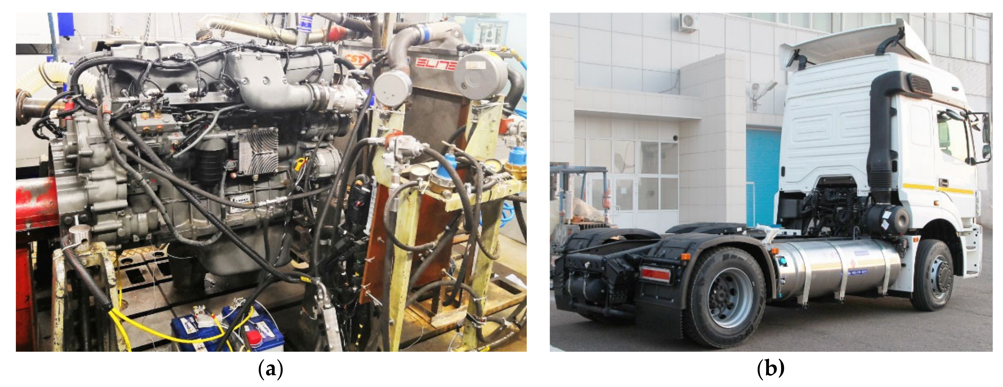
Figure 2.
Parallel hybrid powertrain topology with a stepped automated gearbox. EM: Electric machine, ESS: Energy storage system, ICE: Internal combustion engine.
Figure 2.
Parallel hybrid powertrain topology with a stepped automated gearbox. EM: Electric machine, ESS: Energy storage system, ICE: Internal combustion engine.
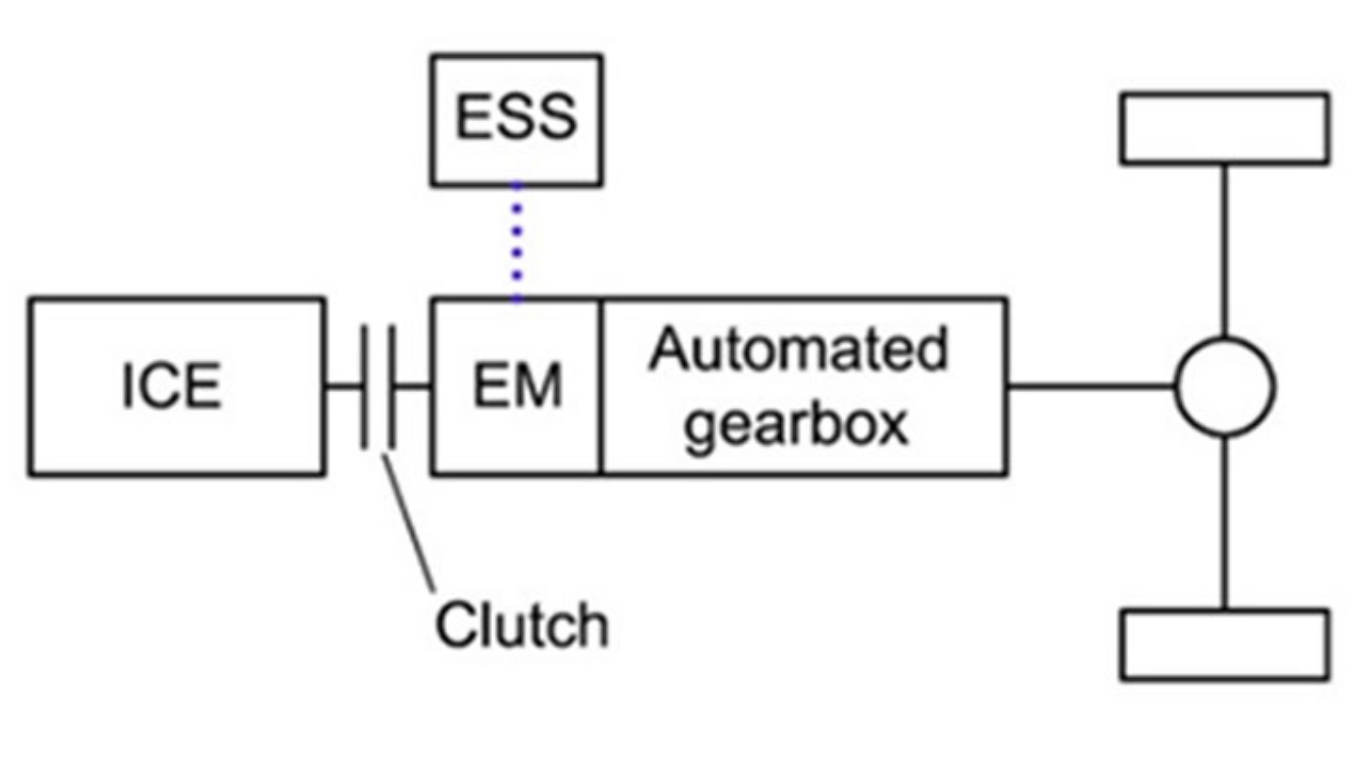
Figure 3.
Brake-specific fuel consumption (BSFC) map of the diesel engine.
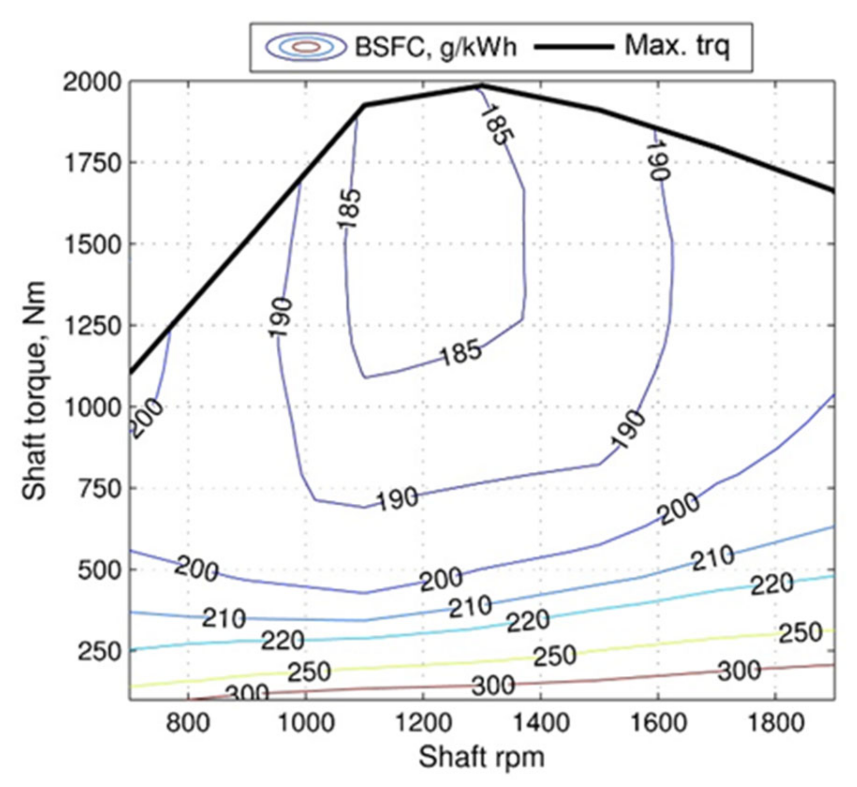
Figure 4.
Brake-specific fuel consumption maps of the developed gas engines: (a) Otto’s cycle and (b) Miller’s cycle.
Figure 4.
Brake-specific fuel consumption maps of the developed gas engines: (a) Otto’s cycle and (b) Miller’s cycle.
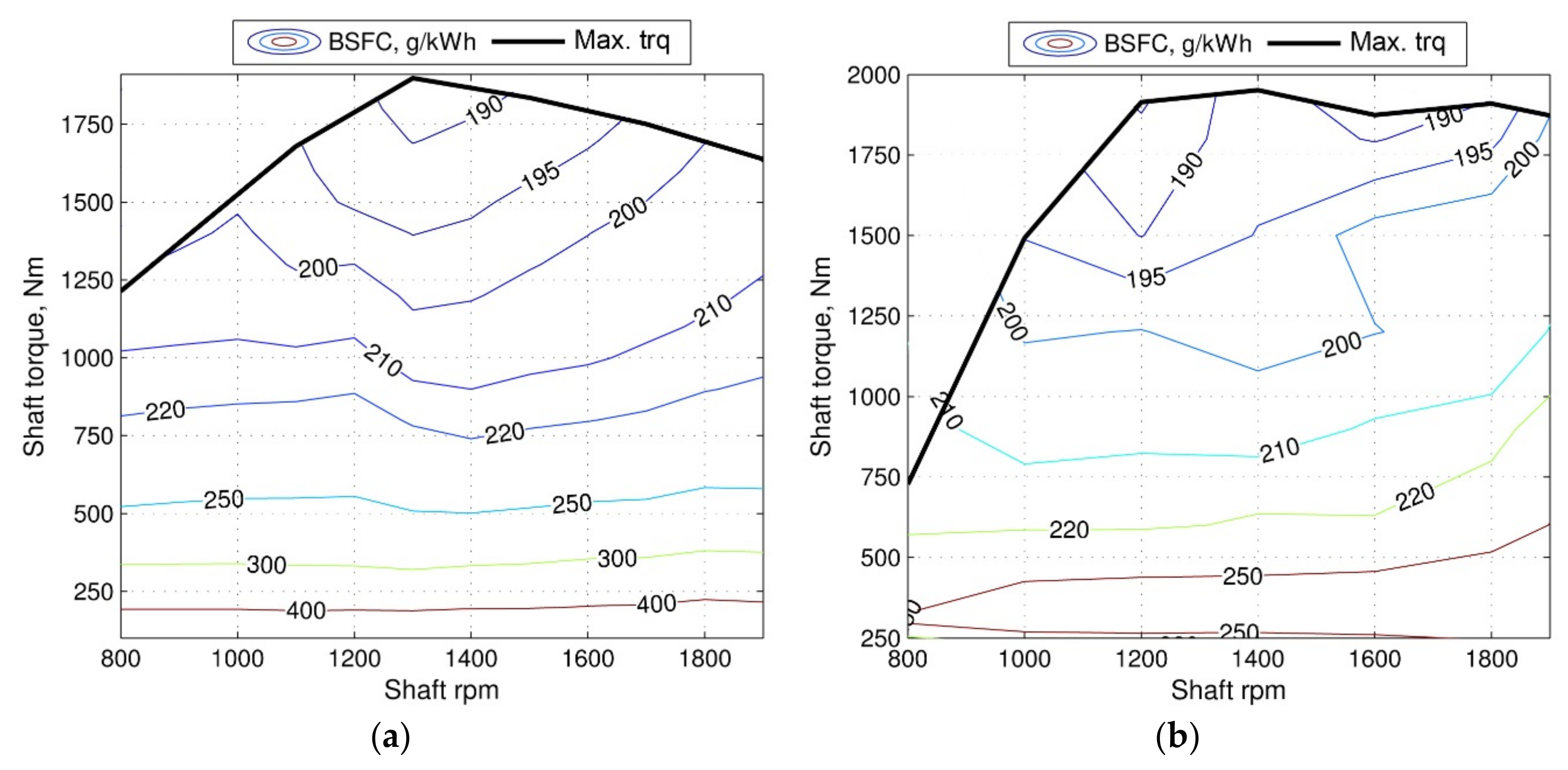
Figure 5.
Efficiency map and torque characteristics of the electric drive (motor mode).
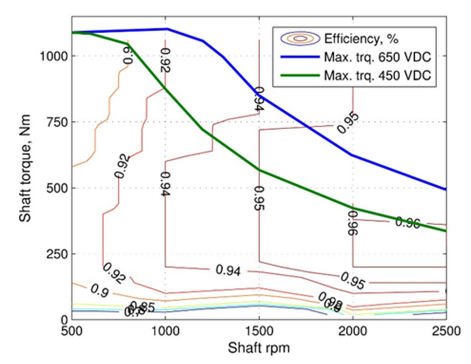
Figure 6.
Equivalent circuit for a supercapacitor.
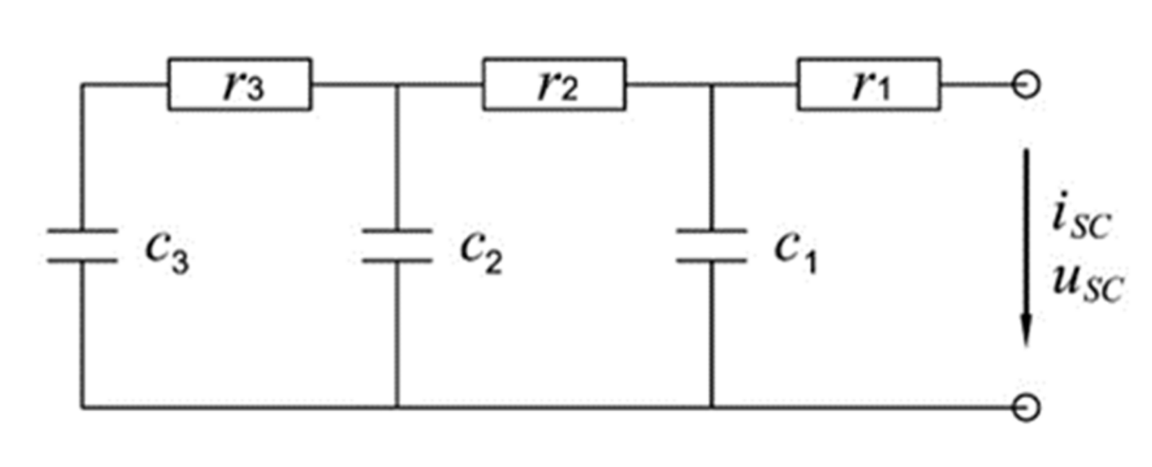
Figure 7.
Comparison of the supercapacitor simulation results with the experimental data.

Figure 8.
Model analysis of the power losses and efficiency of the supercapacitor.

Figure 9.
A simplified diagram of the hybrid powertrain operating modes.

Figure 10.
Superimposed torque characteristics of the hybrid unit and its components.
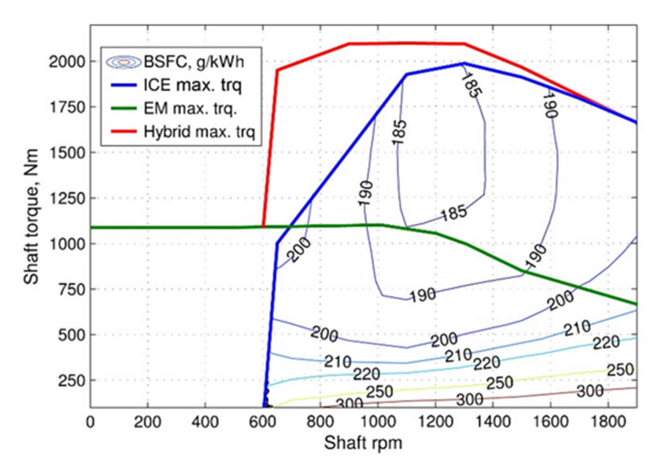
Figure 11.
Driving cycles employed in the simulations. (a,b) velocity and road slope of the World Harmonized Vehicle Cycle (WHVC), (c) the West Virginia University city cycle (WVUCITY), (d) the West Virginia University suburban cycle (WVUSUB), (e) the GOST city cycle (GOST city), (f) the GOST highway cycle (GOST highway).

Figure 12.
Hybrid powertrain operating variables calculated in the World Harmonized Vehicle Cycle (WHVC) (fragment).
Figure 12.
Hybrid powertrain operating variables calculated in the World Harmonized Vehicle Cycle (WHVC) (fragment).
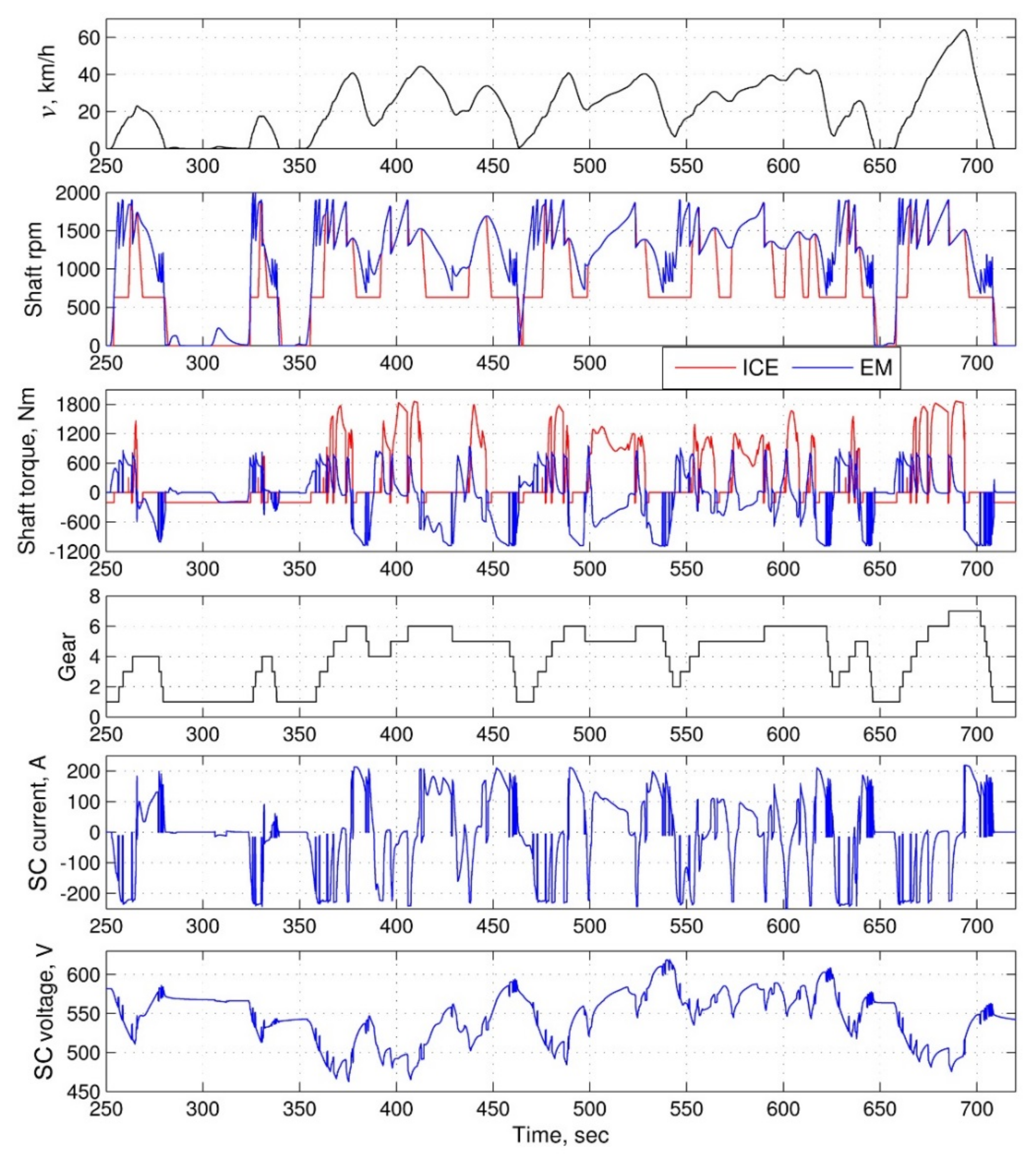
Figure 13.
Supercapacitor voltage dynamics depending on the ESS energy content.

Figure 14.
Influence of the ESS energy content on the supercapacitor efficiency and relative fuel economy.
Figure 14.
Influence of the ESS energy content on the supercapacitor efficiency and relative fuel economy.
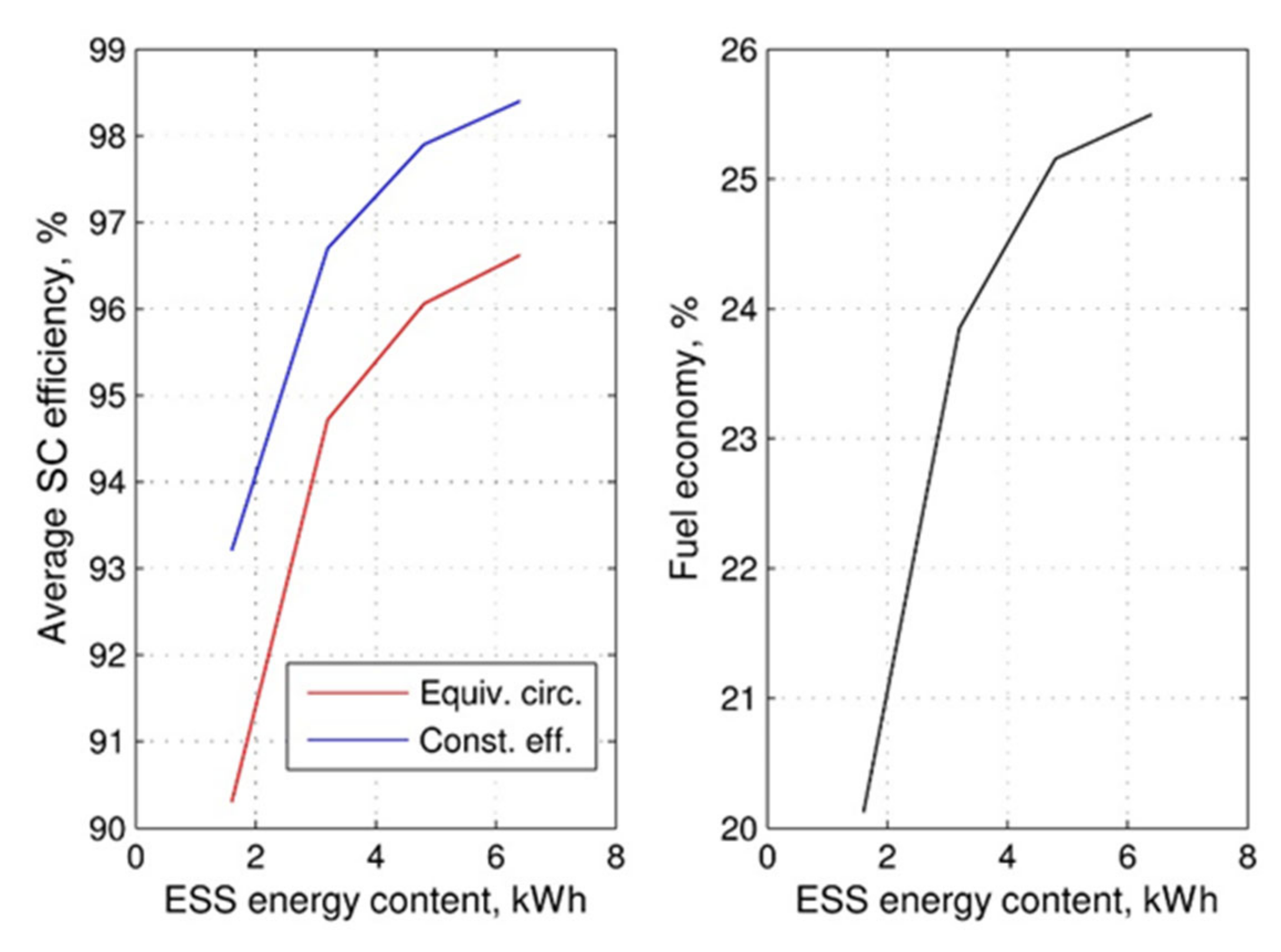
Figure 15.
Calculated fuel economy of the HEV relative to the conventional vehicle: (a) city and suburban cycles, the start–stop was disabled; (b) city and suburban cycles, the start–stop was enabled; and (c) highway cycles.
Figure 15.
Calculated fuel economy of the HEV relative to the conventional vehicle: (a) city and suburban cycles, the start–stop was disabled; (b) city and suburban cycles, the start–stop was enabled; and (c) highway cycles.

Table 1.
The main performance parameters of the traction electric drive.
| DC Voltage (V) | Motor Mode | Generator Mode | ||
|---|---|---|---|---|
| Max. Power (kW) | Max. Torque (Nm) | Max. Power (kW) | Max. Torque (Nm) | |
| 450 | 90 | 1100 | 100 | 1100 |
| 650 | 135 | 1100 | 165 | 1100 |
Table 2.
Supercapacitor equivalent circuit parameters.
| 0.17 | 0.35 | 1.8 | 12 | 8 | 8 |
Table 3.
Power and duty cycle parameters of the auxiliary loads in a conventional HD powertrain.
| Auxiliary Component | Min. Power (kW) | Max. Power (kW) | (%) (Urban Driving) | (%) (Highway Driving) | |
|---|---|---|---|---|---|
| Air brake compressor | 0.35–1.2 | 1–3.5 | 100 | 30 | 5 |
| Power steering | 0.3–1.2 | 3–10.5 | 100 | 60 | 10 |
| A/C compressor | 0 | 1–5.3 | 150 | 50 | 50 |
| Engine fan | 0 | 16.7 | 200 | 10 | 5 |
| Electrical acc. | 0.6 | 0.6 | - | - | - |
Table 4.
Power and duty cycle parameters of the auxiliary loads in the hybrid HD powertrain.
| Auxiliary Component | Power (kW) (Urban Driving) | Power (kW) (Highway Driving) | (%) (Urban Driving) | (%) (Highway Driving) | |
|---|---|---|---|---|---|
| Air brake compressor | 1.7 | 2.2 | 100 | 5 | 5 |
| Power steering | 5.5 | 3 | 100 | 60 | 10 |
| A/C compressor | 2.5 | 3.3 | 150 | 50 | 50 |
| Engine fan | 2.4 | 5.5 | 200 | 4 | 4 |
| Electrical acc. | 0.6 | 0.6 | - | - | - |
| HV cooling | 0.3 | 0.3 | 100 | 56 | 10 |
Table 5.
Basic conditions for the transitions between the hybrid powertrain modes.
| Condition No. | C1 | C2 | C3 | C4 | C5 | C6 |
|---|---|---|---|---|---|---|
| Expression | no gear shift | gear shift |
Table 6.
Parameters of the model of vehicle dynamics.
| (m2) | ||||||
|---|---|---|---|---|---|---|
| 44,000 | 0.492 | 20 | 0.58 | 7.9 | 0.0045 | (1.5–2) × 10−6 |
Table 7.
Comparison between the experimental and calculated fuel economy for the vehicles equipped with the conventional powertrains.
Table 7.
Comparison between the experimental and calculated fuel economy for the vehicles equipped with the conventional powertrains.
| Driving Cycle (GOST) | Fuel Economy, Diesel (L/100 km) | Fuel Economy, Gas-Otto (m3/100 km) | Fuel Economy, Gas, Prod. Engine (m3/100 km) | ||||||
|---|---|---|---|---|---|---|---|---|---|
| Exp. | Model | Error (%) | Exp. | Model | Error (%) | Exp. | Model | Error (%) | |
| City | 58.3 | 58.5 | 0.34 | 74.38 | 72.4 | 2.66 | 61.6 | 67.38 | 9.38 |
| Highway | 35.8 | 37.5 | 4.75 | 46.98 | 46.09 | 1.89 | 43.3 | 42.96 | 0.79 |
Table 8.
Influence of the ESS energy content and the DC interface on the HEV fuel economy.
| ESS–Traction Drive Interface | Powertrain Type | ||||||||
|---|---|---|---|---|---|---|---|---|---|
| Conv. | Hybrid, ESS 1.6 kWh | Hybrid, ESS 3.2 kWh | Hybrid, ESS 4.8 kWh | Hybrid, ESS 6.4 kWh | |||||
| FC | FC | FE | FC | FE | FC | FE | FC | FE | |
| Direct link | 82.6 | 65.98 | 20.12% | 62.9 | 23.8% | 61.82 | 25.16% | 61.54 | 25.50% |
| DC–DC | 70.2 | 15% | 66.95 | 18.9% | 65.7 | 20.46% | 64.98 | 21.33% | |
FC in m3/100 km.
Table 9.
Average hybridization effect of the gas-based powertrains relative to the diesel-based powertrain.
Table 9.
Average hybridization effect of the gas-based powertrains relative to the diesel-based powertrain.
| Driving Schedule | Start–Stop Feature Status | Gas Engine | ||
|---|---|---|---|---|
| Otto’s Cycle | Miller’s Cycle | Production Engine | ||
| City/suburban | Disabled | + 0.7% | −0.6% | −0.7% |
| City/suburban | Enabled | + 3% | + 1.2% | + 0.7% |
| Highway | n/a | + 0.5% | 0 | −0.5% |
Table 10.
Variations of the average fuel-saving effect due to the decreased vehicle mass.
| Driving Schedule | Start–Stop Feature Status | Engine | |||
|---|---|---|---|---|---|
| Diesel | Gas, Otto Cycle | Gas, Miller Cycle | Gas, Prod. Engine | ||
| City/suburban | Disabled | −0.1% | + 0.7% | + 0.4% | + 1.2% |
| City/suburban | Enabled | + 1% | + 1.3% | −0.3% | + 0.2% |
| Highway | n/a | −0.2% | + 0.1% | −0.9% | 0 |
© 2020 by the authors. Licensee MDPI, Basel, Switzerland. This article is an open access article distributed under the terms and conditions of the Creative Commons Attribution (CC BY) license (http://creativecommons.org/licenses/by/4.0/).
Share and Cite
MDPI and ACS Style
Kulikov, I.; Kozlov, A.; Terenchenko, A.; Karpukhin, K. Comparative Study of Powertrain Hybridization for Heavy-Duty Vehicles Equipped with Diesel and Gas Engines. Energies 2020, 13, 2072. https://doi.org/10.3390/en13082072
AMA Style
Kulikov I, Kozlov A, Terenchenko A, Karpukhin K. Comparative Study of Powertrain Hybridization for Heavy-Duty Vehicles Equipped with Diesel and Gas Engines. Energies. 2020; 13(8):2072. https://doi.org/10.3390/en13082072
Chicago/Turabian StyleKulikov, Ilya, Andrey Kozlov, Alexey Terenchenko, and Kirill Karpukhin. 2020. "Comparative Study of Powertrain Hybridization for Heavy-Duty Vehicles Equipped with Diesel and Gas Engines" Energies 13, no. 8: 2072. https://doi.org/10.3390/en13082072
Note that from the first issue of 2016, this journal uses article numbers instead of page numbers. See further details here.