A Super Twisting Fractional Order Terminal Sliding Mode Control for DFIG-Based Wind Energy Conversion System


1
School of Electrical and Electronics Engineering, Chung-Ang University, Dongjak-gu, Seoul 06974, Korea
2
Department of Electrical and Computer Engineering, Comsats University Islamabad, Abbottabad Campus, Abbottabad 22060, Pakistan
3
CECOS University of IT and Emerging Sciences, Peshawar 25100, Pakistan
4
Department of Electrical Engineering, College of Engineering, Taif University KSA, Taif 21974, Saudi Arabia
*
Author to whom correspondence should be addressed.
Energies 2020, 13(9), 2158; https://doi.org/10.3390/en13092158
Submission received: 29 March 2020
/
Revised: 16 April 2020
/
Accepted: 24 April 2020
/
Published: 1 May 2020
(This article belongs to the Special Issue Feedback Control of Wind and Water Turbines)
Abstract
:The doubly fed induction generator (DFIG)-based wind energy conversion systems (WECSs) are prone to certain uncertainties, nonlinearities, and external disturbances. The maximum power transfer from WECS to the utility grid system requires a high-performance control system in the presence of such nonlinearities and disturbances. This paper presents a nonlinear robust chattering free super twisting fractional order terminal sliding mode control (ST-FOTSMC) strategy for both the grid side and rotor side converters of 2 MW DFIG-WECS. The Lyapunov stability theory was used to ensure the stability of the proposed closed-loop control system. The performance of the proposed control paradigm is validated using extensive numerical simulations carried out in MATLAB/Simulink environment. A detailed comparative analysis of the proposed strategy is presented with the benchmark sliding mode control (SMC) and fractional order terminal sliding mode control (FOTSMC) strategies. The proposed control scheme was found to exhibit superior performance to both the stated strategies under normal mode of operation as well as under lumped parametric uncertainties.
1. Introduction
Since the early 20th century, energy from wind has been utilized to add mechanical power to grind grains or to pump water. The first wind turbine was developed to generate electricity. Wind power was remarked as one of the promising renewable energy sources in the decade 1980–1990 [1]. During the end of the 20th century, the capacity of wind energy has approximately increased twice every three years worldwide. At present, windmills, wind-pumps and wind power plants are effectively working in many countries around the world. Since the early 1980, the cost of electricity generated from wind energy has decreased about one-sixth and the trend seems to continue, for example, in 1982, the average list price of Danish-produced wind turbines was 1770 US$/kW, and in 1997, the average price was 850 US$/kW [1]. The use of wind energy does not cause harmful emissions like greenhouse gases during its operating period and, without any surprise, worldwide wind power is one of the rapidly growing renewable energy sources. According to the World Wind Association, wind capacity over the world has reached up to 597 GW in 2019 [2], which was 318 MW in 2013 [3]. The overall capacity for the past seven years is shown in Figure 1. Owing to this increase, the manufacturers are striving to develop wind turbines with a high capacity of 3–6 MW [4]. The wind energy conversion system (WECS) basically comprises an AC generator, gears, and a wind turbine to extract the maximum power from wind energy and transfer to the AC grid. Doubly fed induction generators (DFIGs) are widely used to extract the energy from the wind with the advantages of resilient structure, wide range speed operation capability, low inverter cost [5], active and reactive power control capability in the four-quadrant region, and torque control. Variable control of the DFIG under varying wind speed is necessary to reduce the stresses on mechanical structures and acoustic noises that are the result of high fluctuations in the electromagnetic torque.
The development of a DFIG-based WECS control system is a trivial task. Researchers had already invested in developing a robust control paradigm to improve the performance of the closed-loop DFIG-based WECS. A proportional integral (PI) controller has been widely used as a linear controller for the speed and power control of the DFIG-based WECS. The family of linear controllers—including (1) repetitive control paradigms, (2) deadbeat control, and (3) proportional resonant control—is prone to various problems of robustness and speed convergence under modeled and unmodeled disturbances. A number of nonlinear control techniques have been proposed in the literature in order to cope with the problems of linear controllers. The most recent and prominent control techniques include (1) predictive power control, (2) H-infinity control, (3) fuzzy control, (4) artificial neural network (ANN), (5) sliding mode control (SMC), and (6) hybrid SMC techniques.
A predictive direct torque control (DTC) strategy has been proposed in [6] to reduce the torque ripples and flux ripples of the DFIG. A grid-connected strategy was adopted with constant switching frequency using a two-level voltage source converter (VSI). The authors in [7] have proposed a predictive power paradigm for the DFIG-WECS, in which the voltage was calculated directly from the power prediction variation. The accuracy and robustness of the proposed system have been improved by using switching delay compensation methodologies. The predictive control strategies for WECS have been improved by the introduction of optimization schemes. A constrained genetic algorithm (GA) has been proposed in [8] for the DFIG-based WECS. The weighting factors have been determined using a novel GA, and thus provided a better solution for constrained problems in the DFIG systems. The predictive control-based strategies provided a better solution, but these techniques were prone to computational problems. Comparative analysis of controller with SMC and exact feedback linearization [9] have been made in [10]. The main objective was to mitigate the voltage dips in the DFIG-based WECS and to provide an enhanced fault voltage-ride-through operation. A hybrid controller, combining the features of model predictive control (MPC) and controller, has been presented in [11]. An improved convergence feature was ensured using predictive strategy, while control strategy was used to provide enhanced robustness against external disturbances. Artificial intelligence (AI)-based systems have also been proposed to improve the steady-state response of the DFIG-based WECS. A fuzzy logic controller has been proposed in [12]. The steady-state response was improved and compared with the deadbeat and PI controllers. A hybrid controller based on PI and fuzzy rules has been formulated for the DFIG-WECS [13]. The active and reactive powers were independently controlled and compared with the PI and fuzzy systems. The ANN-based system has also been proposed in the literature. The author in [14] eliminated the flux estimation and inner current loop using ANN based on the rotor loop design. The author in [15] analyzed both the super and sub-synchronous operational modes of the DFIG using ANN at some specific power factor. The adapted control strategy was a field-oriented vector control scheme for the grid side and rotor side converter. A direct power control strategy has been applied in [16] for the DFIG-based WECS using ANN. The direct power control strategy was also proposed in [17] using supervised and fixed models to minimize errors owing to the delay in control time with a shorter execution time. The outcomes from the above ANN-based controller concluded the superior performance over PI-based controllers, but there were certain shortcomings in the execution of ANN. A model-free and intelligent control strategy was proposed in [18]. The authors have addressed the stochastic and nonlinear variations in the DFIG using intelligent control system. The difficulties in ANN were the selection of hidden layers, number of neurons, and selection of suitable rules in the case of fuzzy paradigms.
Apart from these intelligent techniques, variable structure sliding mode control (SMC) has gained increased attention for the DFIG-based WECS owing to its robust nature against both modeled and unmodeled external disturbance, fault scenarios, parameter variations, simple structure, low parameter sensitivity and easy implementation for wind extraction [19], direct power control [20], and maintenance of DC voltage [21]. A number of SMC techniques have been proposed in the literature [22,23,24,25,26]. A novel experimental based SMC has been proposed in [27] using simplified vector control of the DFIG-based WECS. The authors in [28] have proposed an SMC based direct power control strategy to overcome the problem of under-voltage in the DFIG system. The strategy stated was also applied to eliminate the output power oscillation by removing the reactive power ripples interchange in the stator. The control target of achieving symmetrical sinusoidal current in the stator of DFIG was accomplished using an SMC-based power control paradigm. The robustness of the proposed SMC controller was validated using simulation and experimental results on a 2 kW DFIG system. The same strategy has been used in [29] in a discrete-domain to eliminate the power errors through the direct calculation of the rotor voltage. A converter of constant switching frequency was used to simplify the AC harmonic filter design, thus improved the quality of DFIG power in the presence of external distributions and fault scenario. The SMC-based WECS proved to be very robust as compared with previous designed PI-based controllers. The main disadvantage of the classical SMC is the inherently occurring chattering phenomenon owing to the introduction of discontinuous signum function in the control law. A number of hybrid techniques have been proposed in the literature to minimize or completely eliminate the chattering by enhancing the classical SMC. These enhancement techniques include designing different sliding surfaces, reaching law approaches, higher order SMC, and using composite SMC, as shown in Figure 2.
A second-order SMC has been developed in [31,32,33] for DFIG-based WECS. Another second-order SMC has been developed in [34] for the DTC of the DFIG system. The conventional hysteresis control has been replaced with second-order SMC to reduce the flux and torque surface ripples. Classical adapted non-overlapped, fixed, and adjacent horizon adaptation time windows have been revisited with an appropriate receding horizon to model the disturbances and uncertainties due to gusty wind effects. A hybrid SMC has been proposed in [35] through the combination of gravitational search algorithm, its variants, and SMC for DFIG-based WECS. In order to reduce the inherent chattering in the conventional SMC, the author considered the control signals as an objective function [36]. Power flow was performed in [37] using particle swarm optimization based optimized SMC. Another enhancement technique to reduce chattering was the reaching law approach. A number of techniques based on exponential reaching law have been proposed in [38,39,40,41] to reduce chattering with an accelerated approaching process.
All of the above-mentioned techniques are integer order techniques. The recently developed fractional order control paradigm with promising features is widely applied for both nonlinear and linear systems. [42,43]. The authors in [44] present a comprehensive review of the fractional order integration and differentiation. The authors in [45] have proposed that the fractional order control paradigm provided more degree of freedom with respect to integer order control paradigms. The stability of the fractional order paradigm was ensured by proposing fractional order Lyapunov functions in [46]. A number of fractional order control schemes have been proposed for DFIG-based WECS [47,48]. The authors in [48] have compared the fractional order SMC with integer order SMC schemes for WECS. The authors in [49] have proposed an adaptive fractional order terminal SMC (FOTSMC) for DFIG-based WECS, where a comparative analysis of the FOTSMC with the conventional SMC was made. The authors provided simulation-based results to validate the superior performance of the FOTSMC over the conventional SMC in terms of chattering reduction and robustness against external disturbances.
Keeping in view the previous research, a very robust and efficient controller is proposed in this paper by combining the attributes of super twisting SMC (STSMC) and FOTSMC, henceforth called super twisting fractional order terminal SMC (ST-FOTSMC). The performance of the proposed technique is validated through simulations carried out in MATLAB/Simulink, and it has been found to have a superior performance when compared with the benchmark SMC and FOTSMC strategies under the normal mode of operation as well as under lumped parametric uncertainties.
Furthermore, the sectional arrangement of this paper is as follows. The wind turbine and DFIG modeling are presented in Section 2. The control paradigm for the rotor side and grid side converter is presented in Section 3. Section 4 describes the performance evaluation of the proposed control strategy under two different case studies in Matlab/Simulink. Finally, the paper is concluded in Section 5. The basic definitions for fractional calculus are given in Appendix A.
2. DFIG-Based WECS Modeling
This section presents the complete model of the grid side converter, rotor side converters, and wind turbine. The mutual operation of the DFIG-based converters and wind turbine system is shown in Figure 3a.
2.1. Wind Turbine Model
The primary application of a wind turbine is to convert the kinetic energy of wind into mechanical energy. This mechanical energy is expressed in terms of aerodynamic power extracted from the wind. Because the wind speed is stochastic in nature, the power extracted from the wind turbine can never be as much as its total capacity. The aerodynamic power can also be calculated using some special software, as performed in [50].
The aerodynamic power depends on many factors including wind speed and wind turbine geometry, and is given as follows:
where is the air density; R denotes the rotor radius of the wind turbine; is the wind speed; is the power coefficient, which is dependent on the geometry and shape of rotor blades; and and represents the tip speed ratio and pitch angle, respectively, The tip speed ratio is given as:
where is the angular shaft speed of the wind turbine. and are interrelated by a function given as follows:
where , and are positive constants. Referring to Figure 3b, it can be concluded that the maximum power is extracted when , thus giving the maximum value of . The wind turbine torque is expressed as follows:
where represents gear ratio, is generator speed, is the generator torque, and is the aerodynamic torque. Substituting Equation (4) into (1) and (2), the reference generator speed and the reference grid power are given as follows:
where is the efficiency of the wind turbine.
2.2. Doubly Fed Induction Generator Model
It is difficult to represent an asynchronous machine in three phases owing to its strong coupling. A DFIG model in the dq-synchronously reference frame is given below [51]:
where and are the stator voltage components; and are the stator current components; and are the rotor voltage components; and are the rotor current components; and are stator flux components; and are rotor flux components; and are the resistors of the stator and rotor, respectively; and are the rotor and stator angular velocity respectively; and are the inductances of the rotor and stator, respectively; and is the number of pole pairs.
The generator rotating parts dynamics are given by the following:
where is the electromagnetic torque, is the load torque, is the inertia, and F is the viscous friction coefficient. The electromagnetic torque is given as follows:
Aligning the reference frame to the d-axis of stator flux, we have , and thus (8) can be simplified as follows:
Neglecting the per phase stator resistance and making the stature flux constant, and . Using this assumption and substituting (9) in (6) and (7), we get the rotor voltages, active power, and reactive power, given as follows:
Here, and .
The rotor current in terms of stator flux can be given as follows:
3. Rotor Side and Grid Side Converter Control
A robust nonlinear and chattering free ST-FOTSMC-based paradigm is presented in this section. The overall control structure of the DFIG-based WECS works in two loops, which are the outer loop and inner loop control. A cascaded control structure is adopted in WECS control on the basis of the fact that the mechanical subsystem (outer loop) of the DFIG-based WECS is slower than the electrical subsystem (inner loop). The outer loop regulates the speed of the DFIG, while the inner loop regulates the electromagnetic torque and d-axis rotor current.
3.1. Speed Control
The outer loop speed control is formulated using Equation (7) and is given as follows:
where is the control input and is the lumped uncertainty. The speed tracking error is chosen as . Taking the derivative of and substituting from Equation (28) in the derivative of speed error, we get the following:
Using the fractional order calculus, the proposed surface is presented as follows:
The surface derivative is given as follows:
By applying to both sides of Equation (16) and then substituting the value of , we get the following:
The equivalent control law is derived from Equation (17) and the discontinuous control component is designed based on a super twisting control method and is given as follows:
In Equation (18), the term and and represent control gains. To prove that the controller derived in Equation (18) is closed-loop stable, the Lyapunov function is expressed as . Applying the fractional operator to the Lyapunov function yields the following expression [3].
Consider the following inequality [3]:
By combining the Equations (17)–(20), the following expression is obtained.
After simplification, Equation (21) is expressed as follows.
By choosing and such that , the expression is always negative.
3.2. Current Control
The aim of this current control is to derive a controls strategy such that tracks the given reference in the presence of uncertainty. The given current reference trajectory is defined as follows:
Using Equation (9), the reference current is calculated as follows:
The d-axis reference current is derived by substituting , in reference reactive power and is given as follows:
The tracking errors of current are defined as follows:
The error derivative is given as follows:
Hence, Equation (27) can be written as follows:
The proposed sliding surfaces and their first derivatives are given as follows:
Applying to both sides of Equation (30), setting and substituting Equation (28), we get the following:
The equivalent control laws are derived from Equation (31) and the discontinuous control components are designed based on a super twisting control method.
Thus, the complete control law, which is , is deduced from Equation (32). In Equation (32), the constant terms and represent control gains. To prove the closed-loop stability of the controller derived in Equation (32), the Lyapunov function is expressed as . Applying the concept presented in Equation (20) and by applying fractional operator to the Lyapunov function yields the following expression [3].
In Equation (33), and represent positive constants. By combining Equation (31), Equation (32), and Equation (33), the following expression is obtained.
By choosing the constant terms and such that , the expression is always negative.
3.3. Grid Side Control
The magnitude and flow direction of power through the DFIG rotor are not always constant owing to both gusty and sluggish behavior of wind flow. The consistency of the DC link voltage is the key objective of grid side control under the aforementioned circumstances. For this purpose, a vector control strategy is deployed with the orientation of the reference frame along with the grid voltage or stator voltage [3]. Hence, the active and reactive power after and are given as follows:
Equation (35) reveals that the power flow between the grid side converter and grid is proportional to the value of and . The active power flow between the grid and the grid side converter is equal to the DC power. Hence, the dynamics can be expressed as follows:
where E is the DC link voltage. Substituting Equation (36) in Equation (37), we get the following:
The function is expressed as follows:
where is the reference value of , while is the uncertainty term. Substituting from Equation (39) into Equation (38) yields the following:
The voltage tracking error and its derivative are defined as follows:
Replacing from Equation (40) we get the following:
By defining a fractional order surface and its derivative , we have the following:
Applying fractional operator to Equation (44), we have the following:
A simplified equation is obtained by replacing on and substituting the value of from Equation (43) in Equation (46), which yields the following:
The equivalent control law is derived from Equation (46) and the discontinuous control component is designed based on a super twisting control method.
Thus, the complete control law, , is deduced from (47). In Equation (47), the constant terms and represent control gains. To prove the closed-loop stability of the controller derived in Equation (47), the Lyapunov function is expressed as . Applying the concept presented in (20) and by applying fractional operator to the Lyapunov function yields the following expression [3].
In Equation (48), represents a positive constant. By combining Equation (46), Equation (47), and Equation (48), the following expression is obtained.
By choosing and such that , the expression is always negative.
4. Results and Discussion
Numerical simulations were carried out in Matlab/Simulink environment to analyze and validate the effectiveness of the proposed control paradigm. The parameters of the proposed controller were selected using Matlab/Simulink optimization toolbox. The minimization of the objective function was carried out using the criteria of integral absolute error. The authors in [52] have presented the parameter selection criteria using response optimization. The selected values of parameters are given in Table A1. Figure 4 shows the wind speed profile used in the simulation. Two cases are discussed in detail for both the rotor side as well as the grid side converter’s control.
4.1. CASE 1
In this case, the system is supposed to operate in ideal conditions, such that it is not affected by any uncertainty or external disturbance.
Figure 5a shows the speed response of the DFIG for the SMC, FOTSMC, and proposed ST-FOTSMC strategies. The SMC scheme exhibits an oscillatory response owing to inherent chattering. The FOTSMC strategy alleviates chattering through the fractional approach. The proposed ST-FOTSMC scheme offers superior and accurate chattering-free speed tracking to the other two candidates. This is further validated by the speed tracking error , illustrated in Figure 5b, where the speed tracking error is the minimum for the proposed strategy as compared with the SMC and FOTSMC techniques.
The active and reactive power comparisons for the DFIG stator are depicted in Figure 6a,b, respectively. The active power with the SMC controller suffers from the highest oscillations, while the FOTSMC strategy makes these oscillations less severe. Again, the proposed ST-FOTSMC paradigm offers a superior and smooth chattering free active power. The same is true for the reactive power. The FOTSMC strategy takes a certain amount of time to bring the reactive power to zero, but it exhibits less chattering than the SMC strategy. The proposed controller brings the reactive power to zero without any disturbance and oscillations, thus ensuring superior performance to its competitors.
As discussed earlier, the active and reactive powers are controlled through the and components of the stator current, respectively. Figure 7a,b illustrate the tracking errors of the and components of the stator currents, respectively. It is evident from the stated figures that the steady-state current errors, and are the least in the case of the proposed ST-FOTSMC technique, thus validating its superior performance to the other two strategies.
The control inputs comparison for the rotor side controller and the current controller is depicted in Figure 8a, while Figure 8b shows the sliding surfaces comparison for the current controllers and the speed controller. It can be observed that, in each case, the proposed ST-FOTSMC technique has a very fast dynamic response with almost no chattering as compared with the SMC and FOTSMC schemes.
The DC-link voltage is shown in Figure 9a for each candidate. It is evident that the proposed ST-FOTSMC technique maintains a constant DC-link voltage as compared with the SMC and FOTSMC. This is verified by the DC-link voltage error shown in Figure 9b, where the error is almost equal to zero in the case of the ST-FOTSMC. On the hand, the stated error is not zero in the case of the SMC and FOTSMC paradigms. Furthermore, the error is the largest in the case of the conventional SMC.
Moreover, the control input and sliding surface for the grid side controller are shown in Figure 10a,b, respectively. The worst performance of the conventional SMC can be seen in the form of excessive chattering. However, the proposed ST-FOTSMC scheme exhibits a superior and chattering-free performance to both of its competitors.
4.2. CASES 2
The effectiveness of the proposed controller is further tested under parametric uncertainties and external disturbance. A lumped uncertainty is added to the system, which simulates variation in the DFIG parameters and external disturbance. In this case, the total variation in the DFIG parameters and the external disturbance is assumed to be 25%. The mathematical formulation of the lumped uncertainty is expressed as follows:
A similar case is assumed in Section 4.3. It is assumed that a 25% variation in the nominal parameter with sinusoidal disturbance is acting on the grid side controller. The mathematical formulation is expressed as follows:
The addition of the sinusoidal term generally represents the power oscillations of slow frequency in the DFIG system. The reference speed tracking comparison of the conventional SMC, FOTSMC, and ST-FOTSMC is depicted in Figure 11a, which shows that the proposed controller has superior reference speed tracking performance under parameter uncertainties and external disturbances. The corresponding speed tracking error is shown in Figure 11b, which further validates the superior performance of the proposed scheme. The conventional SMC has been found to have the worst performance in terms of severe chattering.
The active and reactive powers of the DFIG under lumped uncertainty are shown in Figure 12a,b, respectively. It can be seen that the proposed ST-FOTSMC technique exhibits chattering-free active and reactive powers compared with the conventional SMC and FOTSMC schemes. Furthermore, the proposed strategy has the fastest convergence in the case of the reactive power.
The current error convergence analysis of the stator and components under lumped uncertainty is shown in Figure 13a,b, respectively. It is evident that the proposed scheme converges the stated errors to zero much faster than both the conventional SMC and FOTSMC schemes, with almost no chattering. On the other hand, chattering can be seen in both the conventional SMC and FOTSMC schemes. This validates the superior performance of the proposed technique under lumped uncertainties.
The DC-link voltage and the corresponding DC-link voltage error under lumped uncertainties are shown in Figure 14a,b, respectively. The proposed control scheme exhibits superior performance to the other candidates by maintaining a chattering-free DC-link voltage with the least error.
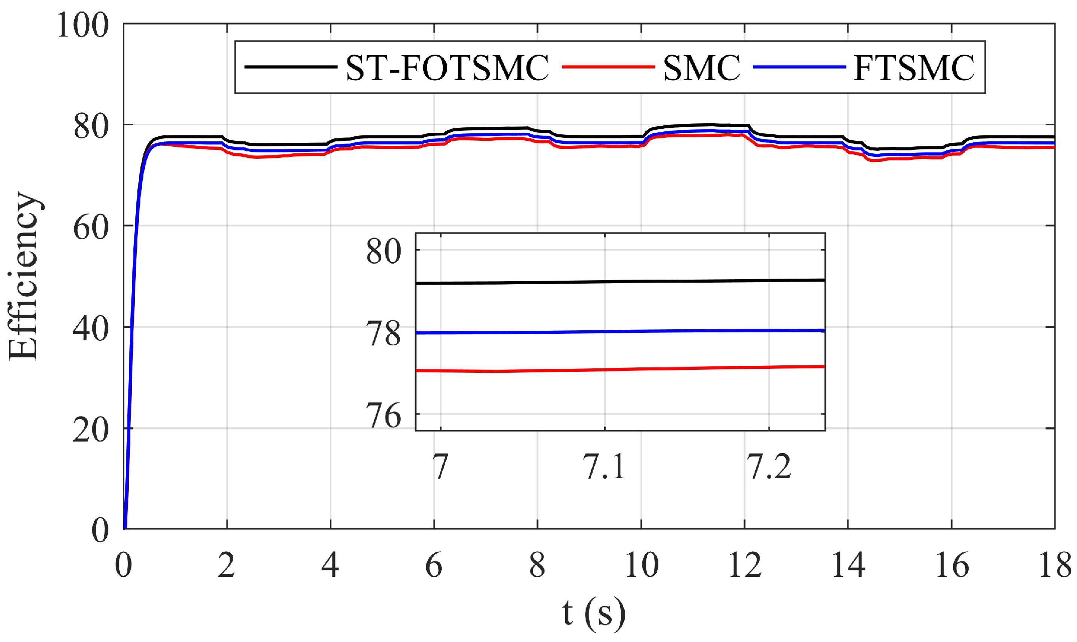
4.3. Efficiency
The appropriate control of DFIG-based WECS is essential for efficiency enhancement of the system. The efficiency of the DFIG-based WECS is the ratio of the active power injected into the grid to the available wind power. The efficiency of the system under consideration is given as follows [53]:
where is the active power injected into the grid given in Equation (35) and is shown in Figure 6a. The wind, , is calculated as follows:
where is the density of air, is the wind speed, and is the wind turbine rotor area. The efficiency of the DFIG for the conventional SMC, FOTSMC, and ST-FOTSMC schemes is compared in Figure 15. It can be observed that the efficiency of the proposed controller reaches up to 80%, which is higher than the efficiencies of both the conventional SMC and FOTSMC schemes. This improvement in efficiency validates the superior performance of the proposed ST-FOTSMC strategy for DFIG-based WECS.
5. Conclusions
By combining the attributes of super twisting SMC and fractional order terminal SMC strategies, a new nonlinear super twisting algorithm based fractional order terminal SMC strategy was proposed in this paper for a utility grid-connected 2 MW DFIG-WECS. The proposed controller is compared with the other two existing variants of the SMC, including the conventional SMC and fractional order terminal SMC, proposed earlier in the literature. Both the stated variants of the SMC and proposed controller are compared with each other under two different cases including normal mode of operation and operation under lumped parametric uncertainties. The numerical simulations carried out in MATLAB/Simulink validate the superior performance of the proposed controller under each condition in terms of minute chattering, fast dynamic response, and fast convergence.
Author Contributions
I.S. and N.U. developed the concept; I.S. and S.U. performed the simulation work, I.S. wrote the paper; Z.A. analyzed the data; J.-S.R. supervised the project. These authors contributed equally to this work. All authors have read and agreed to the published version of the manuscript.
Funding
This research was supported by Basic Science Research Program through the National Research Foundation of Korea funded by the Ministry of Education (2016R1D1A1B01008058) and by Human Resources Development (No.20204030200090) of Korean Institute of Energy Technology Evaluation and Planning (KETEP) grant funded by the Korea government Ministry of Trade, Industry, and Energy.
Conflicts of Interest
The author has no conflict of interest.
Appendix A. Basic Definitions for Fractional Calculus
A Fractional operator is defined as follows [46].
The operator denotes the order of the system where R () is the set of real number. A general fractional operator is described by three definitions [46]. The definitions are named as follows: Caputo definition (A2) for (n – 1) < α < n, Grunwald–Letnikov definition (A3), the Riemann–Liouville definition is also formulated in (A4).
Here, h is the representation of step time, n is the first integer larger than ‘‘a’’, and denotes gamma function.
The author in [54,55] has discussed the stability of fractional order system in detail. A complete comparison of fractional order integration and differentiation is presented in [56]. The authors have reviewed the physical and geometrical interpretation of fraction integration and differentiation. A fractional order s (Laplace operator) is usually approximated using the integer order transfer function. A method has been proposed by Oustaloup to approximate a function having a form given as follows:
The rational function to approximate (A5) is given as follows:
where is the gain responsible to make the unit gain of the both sides of (A6) at 1 rad/sec. 2N + 1 is the number of poles and zeros. and , where and denotes the upper limit and lower limit of the approximation frequency, usually chosen as , and thus .

Table A1.
System and controller parameters. DFIG, doubly fed induction generator.
| DFIG and Wind Turbine Parameter | Values | Control Parameters | Values | Control Parameters | Values |
|---|---|---|---|---|---|
| Voltage | 700 V | k | 0.5–5 | c5 | 0.02 |
| No. of pole pairs | 3 | 0.7 | c6 | 5 | |
| Rs | 1.4 Ohm | 0.8 | kr1 | 0.002 | |
| Rr | 1.2 Ohm | 0.1 | kr2 | 0.02 | |
| M | 0.0051839 H | 0.001 | kr3 | 0.006 | |
| Lr = Ls | 0.0053 H | 0.01 | c7 | 0.005 | |
| 0.00015 | 0.2 | c8 | 1 | ||
| J | 765.6 | 0.003 | kr4 | 0.003 | |
| DC Link Voltage (E) | 800 V | 0.001 | |||
| DC Link Capacitor | 0.01 farad | c1 | 0.0015 | ||
| Frequency | 50 Hz | c2 | 5 | ||
| Blade radius | 35 m | c3 | 0.02 | ||
| Gear ratio | 62.5 | c4 | 5 | ||
| 6.325 |
References
- Neij, L. Cost dynamics of wind power. Energy 1999, 24, 375–389. [Google Scholar] [CrossRef]
- Wind Power Capacity Worldwide Reaches 597 GW, 50.1 GW Added in 2018. Available online: https://wwindea.org/information-2/information/ (accessed on 21 April 2020).
- Ullah, N.; Ali, M.A.; Ibeas, A.; Herrera, J. Adaptive fractional order terminal sliding mode control of a doubly fed induction generator-based wind energy system. IEEE Access 2017, 5, 21368–21381. [Google Scholar] [CrossRef]
- Babu, B.C.; Mohanty, K. Doubly-fed induction generator for variable speed wind energy conversion systems-modeling & simulation. Int. J. Comput. Electr. Eng. 2010, 2, 141. [Google Scholar]
- Zaid, M.M.; Ro, J.-S. Switch Ladder modified H-bridge multilevel inverter with novel pulse width modulation technique. IEEE Access 2019, 7, 102073–102086. [Google Scholar] [CrossRef]
- Abad, G.; Rodríguez, M.Á.; Poza, J. Two-level VSC based predictive direct torque control of the doubly fed induction machine with reduced torque and flux ripples at low constant switching frequency. IEEE Trans. Power Electron. 2008, 23, 1050–1061. [Google Scholar] [CrossRef]
- Zhi, D.; Xu, L.; Williams, B.W. Model-based predictive direct power control of doubly fed induction generators. IEEE Trans. Power Electron. 2009, 25, 341–351. [Google Scholar]
- Rodrigues, L.L.; Potts, A.S.; Vilcanqui, O.A.; Sguarezi Filho, A.J. Tuning a model predictive controller for doubly fed induction generator employing a constrained genetic algorithm. IET Electr. Power Appl. 2019, 13, 812–819. [Google Scholar] [CrossRef]
- Madanzadeh, S.; Abedini, A.; Radan, A.; Ro, J.-S. Application of quadratic linearization state feedback control with hysteresis reference reformer to improve the dynamic response of interior permanent magnet synchronous motors. ISA Trans. 2019, 99, 167–190. [Google Scholar] [CrossRef]
- Qin, B.; Sun, H.; Ma, J.; Li, W.; Ding, T.; Wang, Z.; Zomaya, A.Y. robust h∞ control of doubly fed wind generator via state-dependent riccati equation technique. IEEE Trans. Power Syst. 2018, 34, 2390–2400. [Google Scholar] [CrossRef]
- Aidoud, M.; Sedraoui, M.; Lachouri, A.; Boualleg, A. A robustification of the two degree-of-freedom controller based upon multivariable generalized predictive control law and robust H∞ control for a doubly-fed induction generator. Trans. Inst. Meas. Control 2018, 40, 1005–1017. [Google Scholar] [CrossRef]
- Rocha-Osorio, C.; Solís-Chaves, J.; Rodrigues, L.L.; Puma, J.A.; Sguarezi Filho, A. Deadbeat–fuzzy controller for the power control of a Doubly Fed Induction Generator based wind power system. ISA Trans. 2019, 88, 258–267. [Google Scholar] [CrossRef] [PubMed]
- El Azzaoui, M.; Mahmoudi, H. Fuzzy-PI control of a doubly fed induction generator-based wind power system. Int. J. Autom. Control 2017, 11, 54–66. [Google Scholar] [CrossRef]
- Lantewa, N.G.; Magaji, N. Control of doubly fed induction generator of variable speed wind turbine system using neural network. In Proceedings of the 2018 International Conference and Utility Exhibition on Green Energy for Sustainable Development (ICUE), Phuket, Thailand, 24–26 October 2018; pp. 1–6. [Google Scholar]
- Hore, D.; Sarma, R. Neural network–based improved active and reactive power control of wind-driven double fed induction generator under varying operating conditions. Wind Eng. 2018, 42, 381–396. [Google Scholar] [CrossRef]
- Massoum, S.; Meroufel, A.; Youcefa, B.E.; Massoum, A.; Wira, P. Three-level NPC converter-based neuronal direct active and reactive power control of the doubly fed induction machine for wind energy generation. Majlesi J. Electr. Eng. 2017, 11, 25–32. [Google Scholar]
- Douiri, M.R.; Essadki, A.; Cherkaoui, M. Neural networks for stable control of nonlinear dfig in wind power systems. Procedia Comput. Sci. 2018, 127, 454–463. [Google Scholar] [CrossRef]
- Abouheaf, M.; Gueaieb, W.; Sharaf, A. Model-free adaptive learning control scheme for wind turbines with doubly fed induction generators. IET Renew. Power Gener. 2018, 12, 1675–1686. [Google Scholar] [CrossRef] [Green Version]
- Yang, B.; Yu, T.; Shu, H.; Zhang, Y.; Chen, J.; Sang, Y.; Jiang, L. Passivity-based sliding-mode control design for optimal power extraction of a PMSG based variable speed wind turbine. Renew. Energy 2018, 119, 577–589. [Google Scholar] [CrossRef]
- Hu, J.; Nian, H.; Hu, B.; He, Y.; Zhu, Z. Direct active and reactive power regulation of DFIG using sliding-mode control approach. IEEE Trans. Energy Convers. 2010, 25, 1028–1039. [Google Scholar] [CrossRef]
- Davari, M.; Mohamed, Y.A.-R.I. Robust DC-link voltage control of a full-scale PMSG wind turbine for effective integration in DC grids. IEEE Trans. Power Electron. 2016, 32, 4021–4035. [Google Scholar] [CrossRef]
- Da Costa, J.P.; Pinheiro, H.; Degner, T.; Arnold, G. Robust controller for DFIGs of grid-connected wind turbines. IEEE Trans. Ind. Electron. 2010, 58, 4023–4038. [Google Scholar] [CrossRef]
- Sami, I.; Khan, B.; Asghar, R.; Mehmood, C.A.; Ali, S.M.; Ullah, Z.; Basit, A. Sliding mode-based model predictive torque control of induction machine. In Proceedings of the IEEE International Conference on Engineering and Emerging Technologies (ICEET), Lahore, Pakistan, 21–22 February 2019; pp. 1–5. [Google Scholar]
- Kassem, A.M.; Hasaneen, K.M.; Yousef, A.M. Dynamic modeling and robust power control of DFIG driven by wind turbine at infinite grid. Int. J. Electr. Power Energy Syst. 2013, 44, 375–382. [Google Scholar] [CrossRef]
- Ardjoun, S.A.E.M.; Abid, M. Fuzzy sliding mode control applied to a doubly fed induction generator for wind turbines. Turk. J. Electr. Eng. Comput. Sci. 2015, 23, 1673–1686. [Google Scholar] [CrossRef]
- Djoudi, A.; Chekireb, H.; Bacha, S. Low-cost sliding mode control of WECS based on DFIG with stability analysis. Turk. J. Electr. Eng. Comput. Sci. 2015, 23, 1698–1714. [Google Scholar] [CrossRef]
- Barambones, O.; Cortajarena, J.; Alkorta, P.; de Durana, J. A real-time sliding mode control for a wind energy system based on a doubly fed induction generator. Energies 2014, 7, 6412–6433. [Google Scholar] [CrossRef]
- Shang, L.; Hu, J. Sliding-mode-based direct power control of grid-connected wind-turbine-driven doubly fed induction generators under unbalanced grid voltage conditions. IEEE Trans. Energy Convers. 2012, 27, 362–373. [Google Scholar] [CrossRef]
- Pande, V.; Mate, U.; Kurode, S. Discrete sliding mode control strategy for direct real and reactive power regulation of wind driven DFIG. Electr. Power Syst. Res. 2013, 100, 73–81. [Google Scholar] [CrossRef]
- Mohd Zaihidee, F.; Mekhilef, S.; Mubin, M. Robust speed control of PMSM using sliding mode control (SMC)—A review. Energies 2019, 12, 1669. [Google Scholar] [CrossRef] [Green Version]
- Beltran, B.; Benbouzid, M.E.H.; Ahmed-Ali, T. Second-order sliding mode control of a doubly fed induction generator driven wind turbine. IEEE Trans. Energy Convers. 2012, 27, 261–269. [Google Scholar] [CrossRef] [Green Version]
- Evangelista, C.; Valenciaga, F.; Puleston, P. Active and reactive power control for wind turbine based on a MIMO 2-sliding mode algorithm with variable gains. IEEE Trans. Energy Convers. 2013, 28, 682–689. [Google Scholar] [CrossRef]
- Abdeddaim, S.; Betka, A. Optimal tracking and robust power control of the DFIG wind turbine. Int. J. Electr. Power Energy Syst. 2013, 49, 234–242. [Google Scholar] [CrossRef]
- Boudjema, Z.; Taleb, R.; Djeriri, Y.; Yahdou, A. A novel direct torque control using second order continuous sliding mode of a doubly fed induction generator for a wind energy conversion system. Turk. J. Electr. Eng. Comput. Sci. 2017, 25, 965–975. [Google Scholar] [CrossRef] [Green Version]
- Dahiya, P.; Sharma, V.; Naresh, R. Methods, Hybridized gravitational search algorithm tuned sliding mode controller design for load frequency control system with doubly fed induction generator wind turbine. Optim. Control Appl. 2017, 38, 993–1003. [Google Scholar] [CrossRef]
- Kwon, H.-S.; Ro, J.-S.; Jung, H.-K. A novel social insect optimization algorithm for the optimal design of an interior permanent magnet synchronous machine. IEEE Trans. Magn. 2018, 54, 1–6. [Google Scholar] [CrossRef]
- Taleb, M.; Hbib, M.; Cherkaoui, M.; Taleb, M. Power flow control in wind energy conversion systems using PSO optimized adaptive sliding mode control. In 2018 Renewable Energies, Power Systems & Green Inclusive Economy (REPS-GIE); IEEE: Piscataway, NJ, USA, 2018; pp. 1–5. [Google Scholar]
- Mozayan, S.M.; Saad, M.; Vahedi, H.; Fortin-Blanchette, H.; Soltani, M. Sliding mode control of PMSG wind turbine based on enhanced exponential reaching law. IEEE Trans. Ind. Electron. 2016, 63, 6148–6159. [Google Scholar] [CrossRef]
- Belgacem, K.; Mezouar, A.; Essounbouli, N. Design and analysis of adaptive sliding mode with exponential reaching law control for double-fed induction generator based wind turbine. Int. J. Power Electron. Drive Syst. 2018, 9, 1534. [Google Scholar] [CrossRef]
- Liu, Y.; Wang, Z.; Xiong, L.; Wang, J.; Jiang, X.; Bai, G.; Li, R.; Liu, S. DFIG wind turbine sliding mode control with exponential reaching law under variable wind speed. Int. J. Electr. Power Energy Syst. 2018, 96, 253–260. [Google Scholar] [CrossRef]
- Xiong, L.; Li, P.; Li, H.; Wang, J. Sliding mode control of DFIG wind turbines with a fast exponential reaching law. Energies 2017, 10, 1788. [Google Scholar] [CrossRef] [Green Version]
- Chaal, H.; Jovanovic, M. Direct power control of brushless doubly-fed reluctance machines. In Proceedings of the Power Electronics, Machines and Drives (PEMD 2010), 5th IET International Conference, Brighton, UK, 19–21 April 2010. [Google Scholar]
- Bai, J.; Feng, X.-C. Fractional-order anisotropic diffusion for image denoising. IEEE Trans. Image Process. 2007, 16, 2492–2502. [Google Scholar] [CrossRef]
- Miller, K.S.; Ross, B. An Introduction to the Fractional Calculus and Fractional Differential Equations; Wiley: Hoboken, NJ, USA, 1993. [Google Scholar]
- Delghavi, M.B.; Shoja-Majidabad, S.; Yazdani, A. Fractional-order sliding-mode control of islanded distributed energy resource systems. IEEE Trans. Sustain. Energy 2016, 7, 1482–1491. [Google Scholar] [CrossRef]
- Aghababa, M.P. A Lyapunov-based control scheme for robust stabilization of fractional chaotic systems. Nonlinear Dyn. 2014, 78, 2129–2140. [Google Scholar] [CrossRef]
- Ebrahimkhani, S. Robust fractional order sliding mode control of doubly-fed induction generator (DFIG)-based wind turbines. ISA Trans. 2016, 63, 343–354. [Google Scholar] [CrossRef]
- Asghar, M. Performance comparison of wind turbine based doubly fed induction generator system using fault tolerant fractional and integer order controllers. Renew. Energy 2018, 116, 244–264. [Google Scholar] [CrossRef]
- Hosseinabadi, M.; Rastegar, H. DFIG based wind turbines behavior improvement during wind variations using fractional order control systems. Irani J. Electr.and Electron. Eng. 2014, 10, 314–323. [Google Scholar]
- Pashchenko, D. Ansys Fluent CFD modeling of solar air-heater thermoaerodynamics. Appl. Sol. Energy 2018, 54, 32–39. [Google Scholar] [CrossRef]
- Lima, F.; Watanabe, E.H.; Rodriguez, P.; Luna, A. A simplified model for wind turbine based on doubly fed induction generator. In Proceedings of the 2011 International Conference on Electrical Machines and Systems, Beijing, China, 20–23 August 2011; pp. 1–6. [Google Scholar]
- Ullah, N.; Ali, M.A.; Ahmad, R.; Khattak, A. Fractional order control of static series synchronous compensator with parametric uncertainty. IET Gener. Transm. Distrib. 2017, 11, 289–302. [Google Scholar] [CrossRef]
- Mesemanolis, A.; Mademlis, C.; Kioskeridis, I. High-efficiency control for a wind energy conversion system with induction generator. IEEE Trans. Energy Convers. 2012, 27, 958–967. [Google Scholar] [CrossRef]
- Matignon, D. Stability properties for generalized fractional differential systems. ESAIM Proc. 1998, 5, 145–158. [Google Scholar] [CrossRef] [Green Version]
- Zhang, F.; Li, C. Stability analysis of fractional differential systems with order lying in (1, 2). Adv. Differ. Equ. 2011, 2011, 213485. [Google Scholar] [CrossRef] [Green Version]
- Podlubny, I. Geometric and physical interpretation of fractional integration and fractional differentiation. arXiv 2001, arXiv:math/0110241. [Google Scholar]
Figure 1.
Total globally installed wind power capacity (GW) [2].
Figure 1.
Total globally installed wind power capacity (GW) [2].
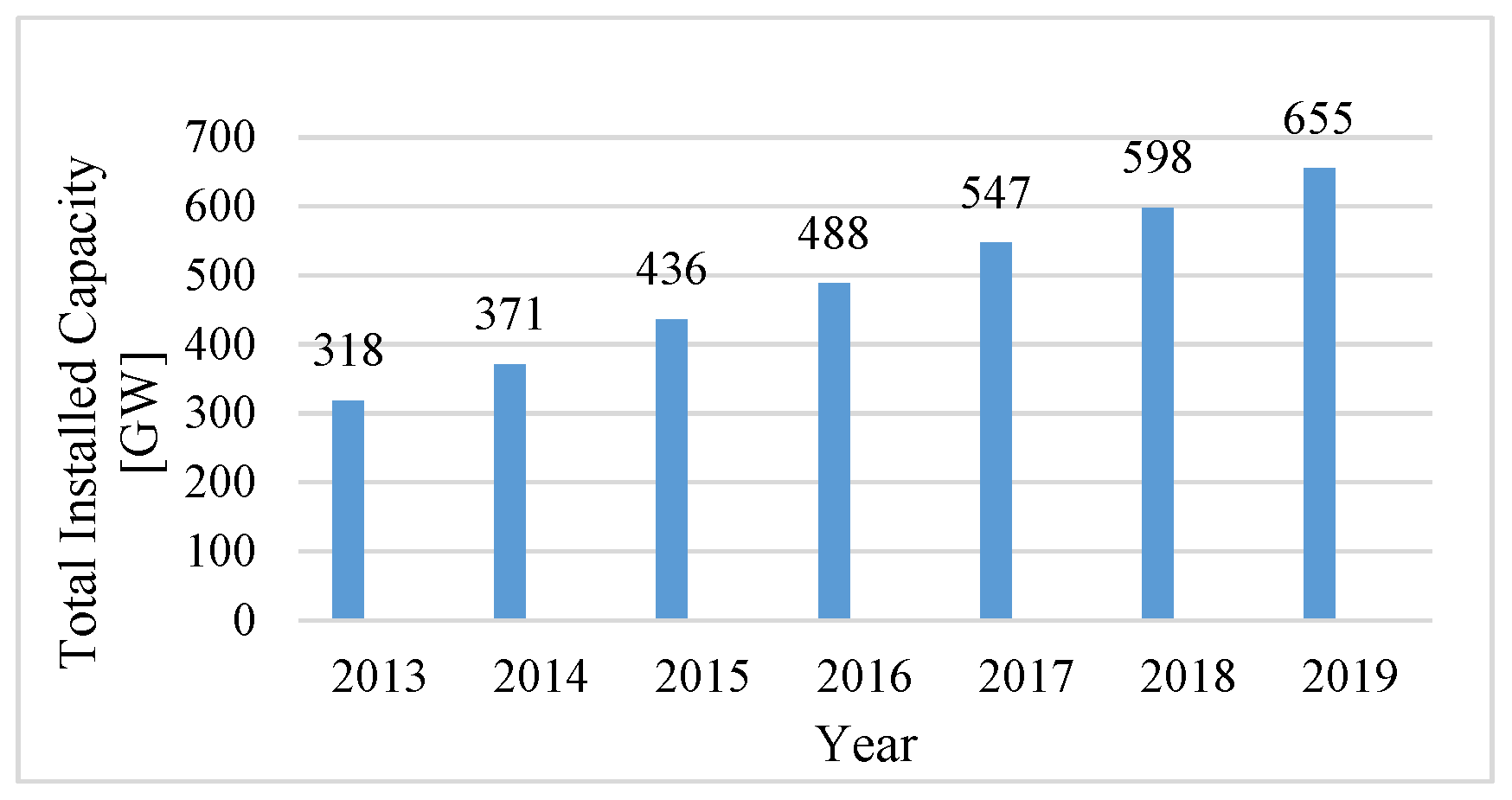
Figure 2.
Enhancement made in sliding mode control (SMC) [30].
Figure 2.
Enhancement made in sliding mode control (SMC) [30].
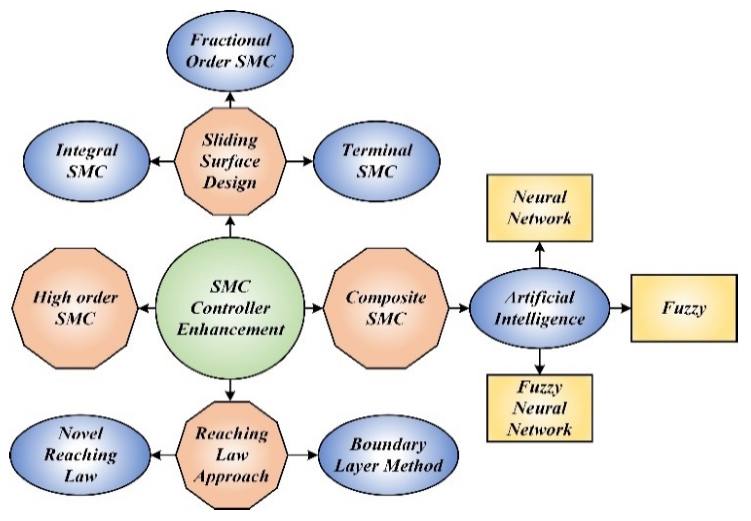
Figure 3.
(a) Schematic of the doubly fed induction generator (DFIG)-based wind energy conversion system (WECS); (b) ideal wind turbine power curve.
Figure 3.
(a) Schematic of the doubly fed induction generator (DFIG)-based wind energy conversion system (WECS); (b) ideal wind turbine power curve.

Figure 4.
Wind speed profile.

Figure 5.
(a) Reference speed tracking comparison under normal conditions; (b) speed error comparison.
Figure 5.
(a) Reference speed tracking comparison under normal conditions; (b) speed error comparison.

Figure 6.
(a) Active power comparison; (b) reactive power comparison.

Figure 7.
(a) under normal conditions; (b) under normal conditions.

Figure 8.
(a) Control inputs comparison; (b) sliding surfaces comparison for rotor side control.

Figure 9.
(a) DC-link voltage; (b) DC-link voltage error comparison under normal conditions.

Figure 10.
(a) Control input for grid side control; (b) grid side control sliding surface.

Figure 11.
(a) Speed response under parametric uncertainties; (b) speed error comparison under lumped uncertainties.
Figure 11.
(a) Speed response under parametric uncertainties; (b) speed error comparison under lumped uncertainties.
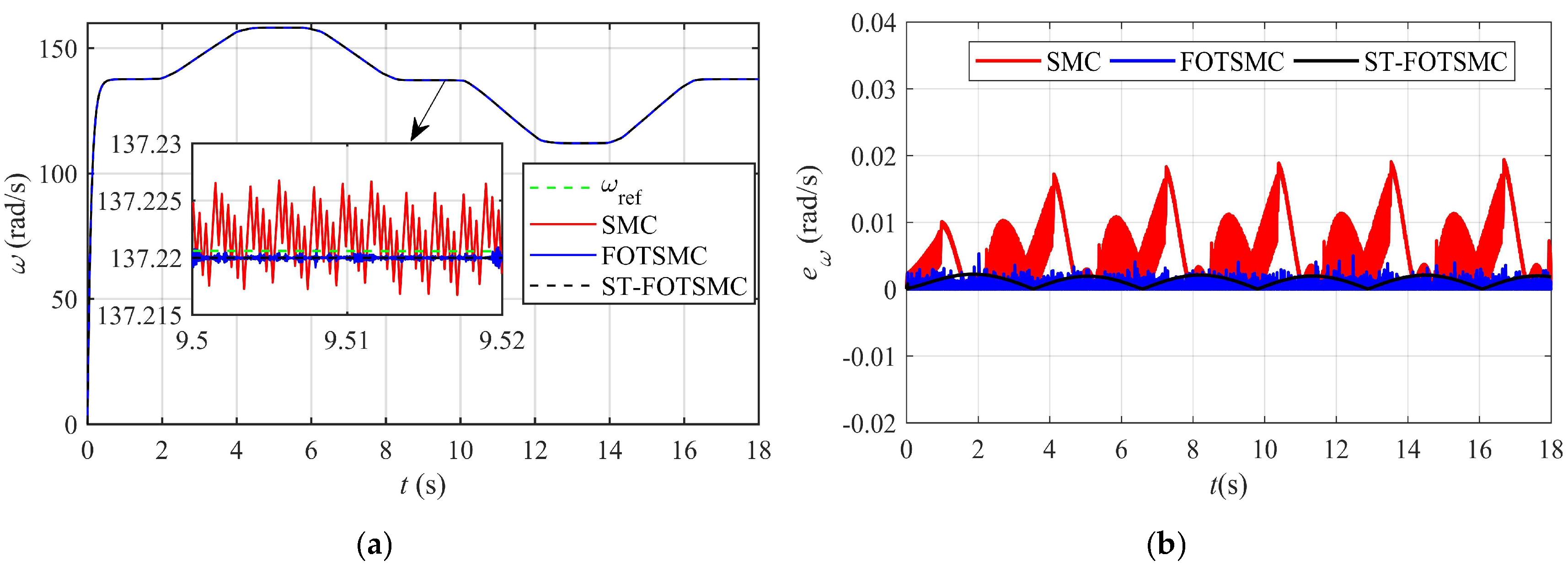
Figure 12.
(a) Active power under lumped disturbances; (b) reactive power comparison under lumped disturbances.
Figure 12.
(a) Active power under lumped disturbances; (b) reactive power comparison under lumped disturbances.
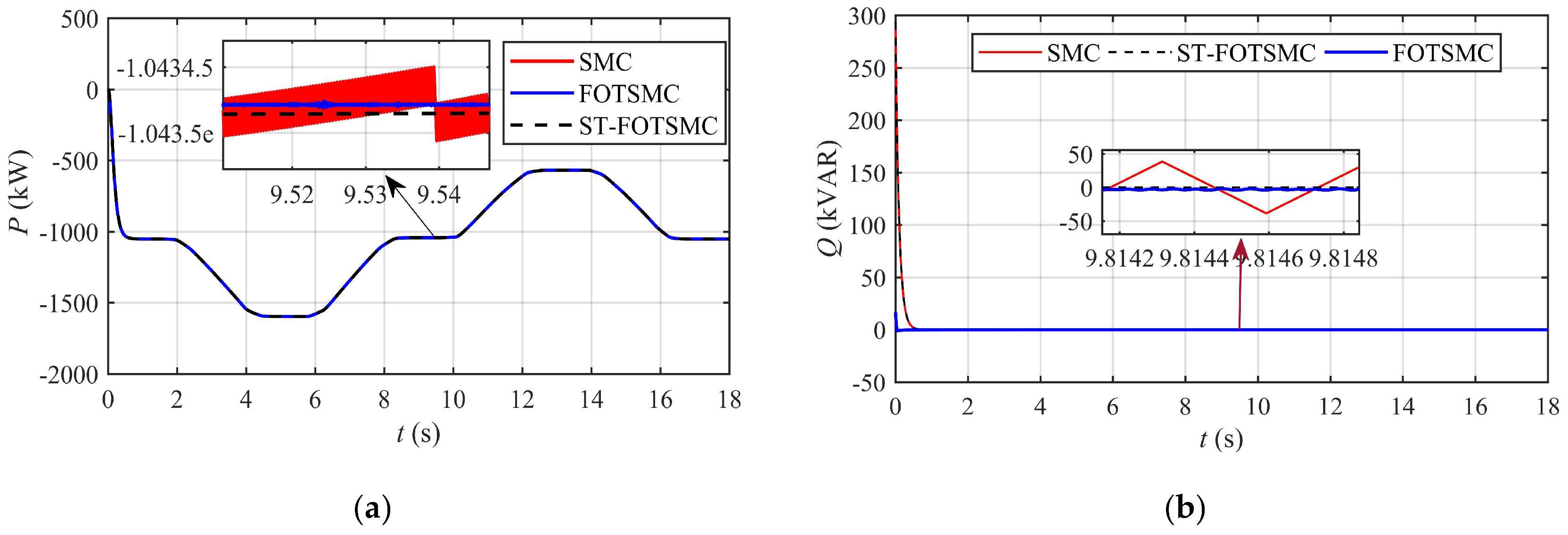
Figure 13.
(a) under lumped uncertainties; (b) under lumped uncertainties.

Figure 14.
(a) DC-link voltage; (b) voltage error under lumped uncertainties.
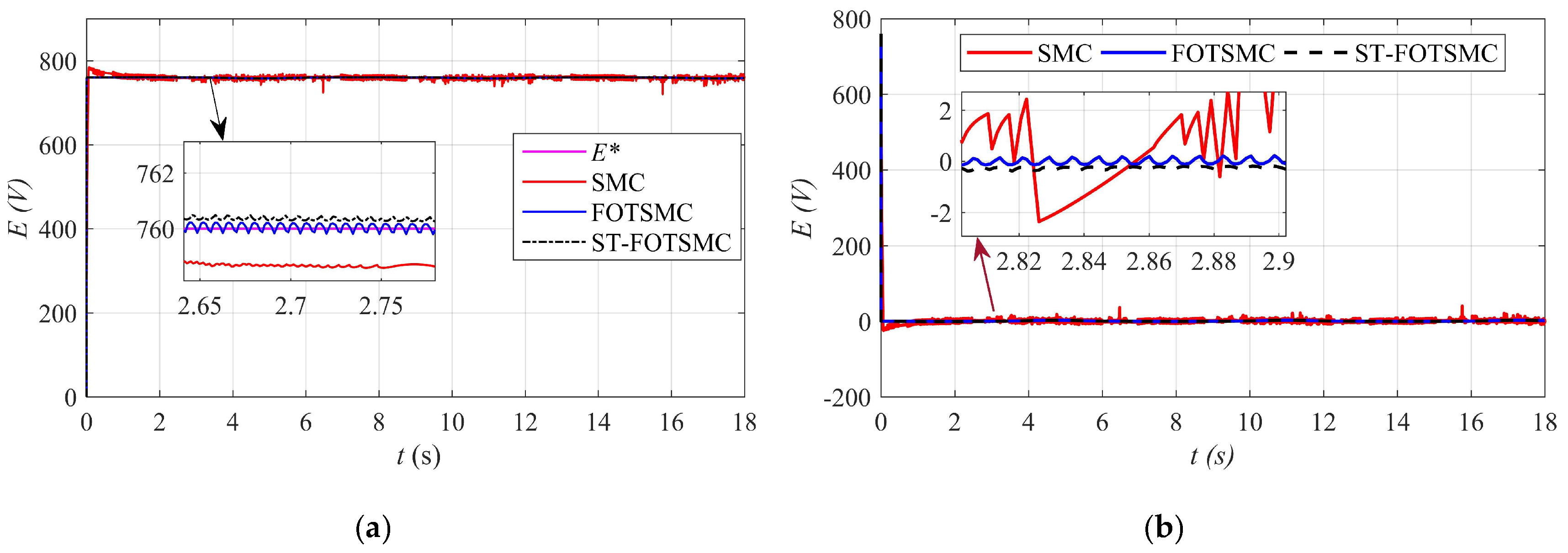
Figure 15.
Efficiency of the DFIG.
© 2020 by the authors. Licensee MDPI, Basel, Switzerland. This article is an open access article distributed under the terms and conditions of the Creative Commons Attribution (CC BY) license (http://creativecommons.org/licenses/by/4.0/).
Share and Cite
MDPI and ACS Style
Sami, I.; Ullah, S.; Ali, Z.; Ullah, N.; Ro, J.-S. A Super Twisting Fractional Order Terminal Sliding Mode Control for DFIG-Based Wind Energy Conversion System. Energies 2020, 13, 2158. https://doi.org/10.3390/en13092158
AMA Style
Sami I, Ullah S, Ali Z, Ullah N, Ro J-S. A Super Twisting Fractional Order Terminal Sliding Mode Control for DFIG-Based Wind Energy Conversion System. Energies. 2020; 13(9):2158. https://doi.org/10.3390/en13092158
Chicago/Turabian StyleSami, Irfan, Shafaat Ullah, Zahoor Ali, Nasim Ullah, and Jong-Suk Ro. 2020. "A Super Twisting Fractional Order Terminal Sliding Mode Control for DFIG-Based Wind Energy Conversion System" Energies 13, no. 9: 2158. https://doi.org/10.3390/en13092158
Note that from the first issue of 2016, this journal uses article numbers instead of page numbers. See further details here.