
National Carbon Accounting—Analyzing the Impact of Urbanization and Energy-Related Factors upon CO2 Emissions in Central–Eastern European Countries by Using Machine Learning Algorithms and Panel Data Analysis

 ,
,  ,
, 
 ,
,
Abstract
:
1. Introduction
2. Materials and Methods
2.1. Dataset Description
2.2. Analysis Methodology
3. Results and Discussion
- CO_2it—CO2 emissions;
- energyit—energy intensity;
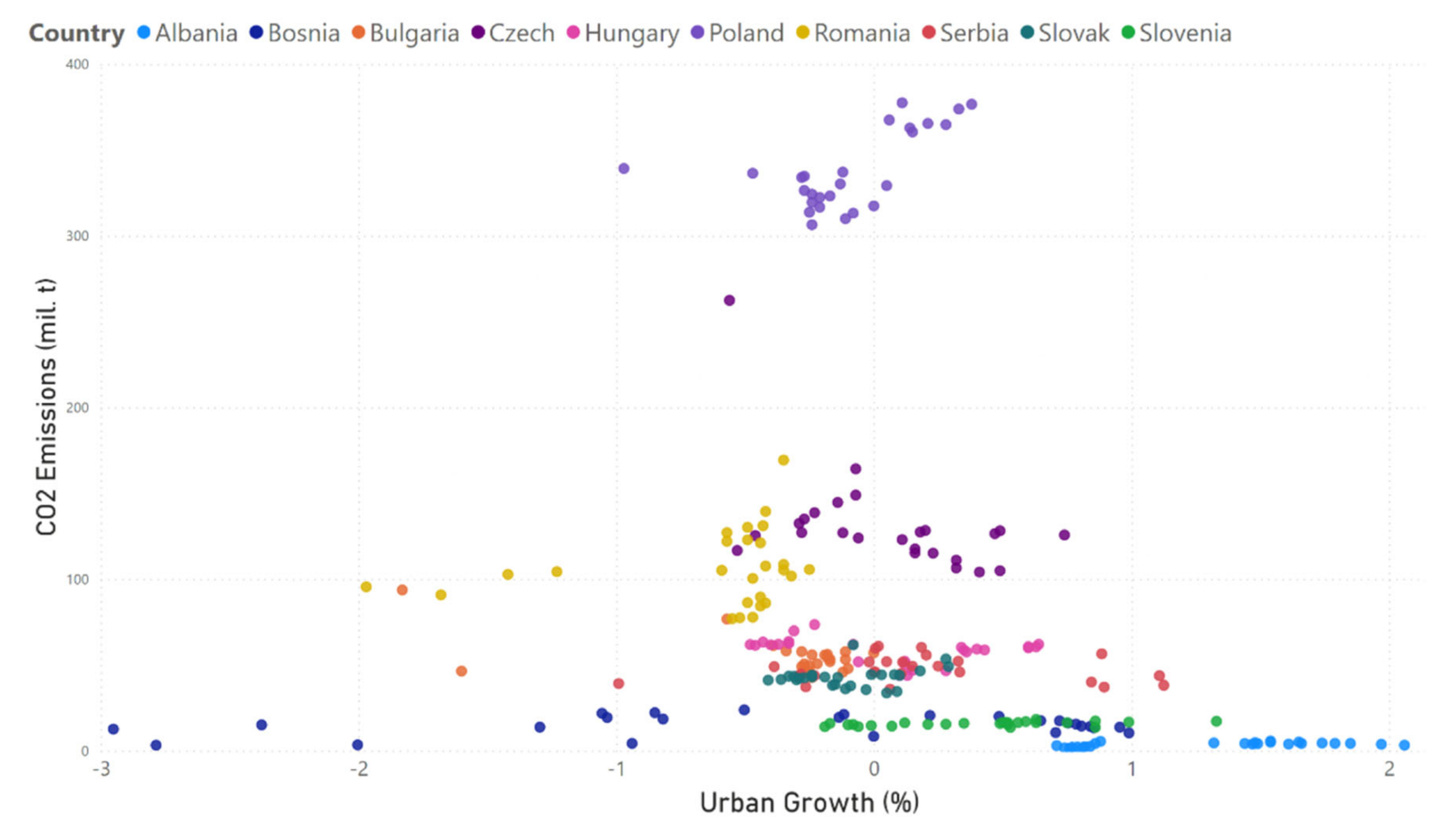
- ugit—urban population growth;
- upit—urban population;
- uit—represents the error, which is composed of three parts: individual-specific unnoticed effect (αi), time-specific unnoticed effect (µ) and individual and time-specific unnoticed effect (εit);
- c—represents the constant or the intercept;
- a1, a2, a3—model parameters to be estimated (their values are other than 0).
4. Discussion and Conclusions
Author Contributions
Funding
Institutional Review Board Statement
Informed Consent Statement
Acknowledgments
Conflicts of Interest
Appendix A

References
- Satterthwaite, D. Cities’ contribution to global warming: Notes on the allocation of greenhouse gas emissions. Environ. Urban. 2008, 20, 539–549. [Google Scholar] [CrossRef] [Green Version]
- Marcotullio, P.J.; Sarzynski, A.; Albrecht, J.; Schulz, N. A Top-Down Regional Assessment of Urban Greenhouse Gas Emissions in Europe. Ambio 2014, 43, 957–968. [Google Scholar] [CrossRef] [PubMed] [Green Version]
- Bader, N.; Bleischwitz, R. Measuring Urban Greenhouse Gas Emissions: The Challenge of Comparability. SAPIENS 2009, 2, 3. Available online: https://journals.openedition.org/sapiens/854 (accessed on 12 February 2021).
- Minnig, M.; Moeck, C.; Radny, D.; Schirmer, M. Impact of urbanization on groundwater recharge rates in Dübendorf, Switzerland. J. Hydrol. 2018, 563, 1135–1146. [Google Scholar] [CrossRef] [Green Version]
- Fang, C.; Liu, H.; Li, G. International progress and evaluation on interactive coupling effects between urbanization and the eco-environment. J. Geogr. Sci. 2016, 26. [Google Scholar] [CrossRef]
- Kurniawan, R.; Managi, S. Coal consumption, urbanization, and trade openness linkage in Indonesia. Energy Policy 2018, 121, 576–583. [Google Scholar] [CrossRef]
- Bai, Y.; Deng, X.; Gibson, J.; Zhao, Z.; Xu, H. How does urbanization affect residential CO2 emissions? An analysis on urban agglomerations of China. J. Clean. Prod. 2019, 209, 876–885. [Google Scholar] [CrossRef]
- Wang, Y.; Zhao, T. Impacts of urbanization-related factors on CO2 emissions: Evidence from China’s three regions with varied urbanization levels. Atmos. Pollut. Res. 2018, 9, 15–26. [Google Scholar] [CrossRef]
- Petrović, N.; Bojović, N.; Petrović, J. Appraisal of urbanization and traffic on environmental quality. J. CO2 Util. 2016, 16, 428–430. [Google Scholar] [CrossRef]
- Kasman, A.; Duman, Y.S. CO2 emissions, economic growth, energy consumption, trade and urbanization in new EU member and candidate countries: A panel data analysis. Econ. Model. 2015, 44, 97–103. [Google Scholar] [CrossRef]
- Wang, Y.; Li, L.; Kubota, J.; Han, R.; Zhu, X.; Lu, G. Does urbanization lead to more carbon emission? Evidence from a panel of BRICS countries. Appl. Energy 2016, 168, 375–380. [Google Scholar] [CrossRef]
- Sheng, P.; Guo, X. The Long-run and Short-run Impacts of Urbanization on Carbon Dioxide Emissions. Econ. Model. 2016, 53, 208–215. [Google Scholar] [CrossRef]
- Wang, Y.; Chen, L.; Kubota, J. The relationship between urbanization, energy use and carbon emissions: Evidence from a panel of Association of Southeast Asian Nations (ASEAN) countries. J. Clean. Prod. 2016, 112, 1368–1374. [Google Scholar] [CrossRef]
- Abbasi, K.R.; Shahbaz, M.; Jiao, Z.; Tufail, M. How energy consumption, industrial growth, urbanization, and CO2 emissions affect economic growth in Pakistan? A novel dynamic ARDL simulations approach. Energy 2021, 221. [Google Scholar] [CrossRef]
- Algarini, A. The relationship among GDP, carbon dioxide emissions, energy consumption, and energy production from oil and gas in Saudi Arabia. Int. J. Energy Econ. Policy 2020, 10. [Google Scholar] [CrossRef]
- Mahmood, H.; Alkhateeb, T.T.Y.; Al-Qahtani, M.M.Z.; Allam, Z.; Ahmad, N.; Furqan, M. Urbanization, oil price and pollution in Saudi Arabia. Int. J. Energy Econ. Policy 2020, 10. [Google Scholar] [CrossRef] [Green Version]
- Hashmi, S.H.; Fan, H.; Habib, Y.; Riaz, A. Non-linear relationship between urbanization paths and CO2 emissions: A case of South, South-East and East Asian economies. Urban Clim. 2021, 37. [Google Scholar] [CrossRef]
- Wang, Z.; Rasool, Y.; Zhang, B.; Ahmed, Z.; Wang, B. Dynamic linkage among industrialisation, urbanisation, and CO2 emissions in APEC realms: Evidence based on DSUR estimation. Struct. Chang. Econ. Dyn. 2020, 52. [Google Scholar] [CrossRef]
- Rauf, A.; Zhang, J.; Li, J.; Amin, W. Structural changes, energy consumption and carbon emissions in China: Empirical evidence from ARDL bound testing model. Struct. Chang. Econ. Dyn. 2018, 47. [Google Scholar] [CrossRef]
- Zhu, H.; Xia, H.; Guo, Y.; Peng, C. The heterogeneous effects of urbanization and income inequality on CO2 emissions in BRICS economies: Evidence from panel quantile regression. Environ. Sci. Pollut. Res. 2018, 25. [Google Scholar] [CrossRef]
- Chen, S.; Jin, H.; Lu, Y. Impact of urbanization on CO2 emissions and energy consumption structure: A panel data analysis for Chinese prefecture-level cities. Struct. Chang. Econ. Dyn. 2019, 49, 107–119. [Google Scholar] [CrossRef]
- Chen, J.; Zhou, C.; Wang, S.; Li, S. Impacts of energy consumption structure, energy intensity, economic growth, urbanization on PM2.5 concentrations in countries globally. Appl. Energy 2018, 230, 94–105. [Google Scholar] [CrossRef]
- He, Z.; Xu, S.; Shen, W.; Long, R.; Chen, H. Impact of urbanization on energy related CO2 emission at different development levels: Regional difference in China based on panel estimation. J. Clean. Prod. 2017, 140, 1719–1730. [Google Scholar] [CrossRef]
- Shahbaz, M.; Haouas, I.; Hoang, T.H. Van Economic growth and environmental degradation in Vietnam: Is the environmental Kuznets curve a complete picture? Emerg. Mark. Rev. 2019, 38, 197–218. [Google Scholar] [CrossRef]
- Wang, Q.; Kwan, M.P.; Zhou, K.; Fan, J.; Wang, Y.; Zhan, D. The impacts of urbanization on fine particulate matter (PM2.5) concentrations: Empirical evidence from 135 countries worldwide. Environ. Pollut. 2019, 247, 989–998. [Google Scholar] [CrossRef]
- Ouyang, X.; Lin, B. Carbon dioxide (CO2) emissions during urbanization: A comparative study between China and Japan. J. Clean. Prod. 2017, 143, 356–368. [Google Scholar] [CrossRef]
- Tatar, A.M. Research on CO Pollution in Urban Areas. Rev. Chim. 2018, 69, 1075–1078. [Google Scholar] [CrossRef]
- Sharif Hossain, M. Panel estimation for CO2 emissions, energy consumption, economic growth, trade openness and urbanization of newly industrialized countries. Energy Policy 2011, 39. [Google Scholar] [CrossRef]
- Wang, Q.; Su, M.; Li, R. Toward to economic growth without emission growth: The role of urbanization and industrialization in China and India. J. Clean. Prod. 2018, 205. [Google Scholar] [CrossRef]
- Yu, C.; Wenxin, L.; Khan, S.U.; Yu, C.; Jun, Z.; Yue, D.; Zhao, M. Regional differential decomposition and convergence of rural green development efficiency: Evidence from China. Environ. Sci. Pollut. Res. 2020, 27. [Google Scholar] [CrossRef]
- Zhang, G.; Zhang, N.; Liao, W. How do population and land urbanization affect CO2 emissions under gravity center change? A spatial econometric analysis. J. Clean. Prod. 2018, 202. [Google Scholar] [CrossRef]
- Lei, D.; Xu, X.; Zhang, Y. Analysis of the dynamic characteristics of the coupling relationship between urbanization and environment in Kunming city, southwest China. Clean. Environ. Syst. 2021, 2. [Google Scholar] [CrossRef]
- Wang, Y.; Li, X.; Kang, Y.; Chen, W.; Zhao, M.; Li, W. Analyzing the impact of urbanization quality on CO2 emissions: What can geographically weighted regression tell us? Renew. Sustain. Energy Rev. 2019, 104, 127–136. [Google Scholar] [CrossRef]
- Shafiei, S.; Salim, R.A. Non-renewable and renewable energy consumption and CO2 emissions in OECD countries: A comparative analysis. Energy Policy 2014, 66, 547–556. [Google Scholar] [CrossRef] [Green Version]
- Dong, F.; Wang, Y.; Su, B.; Hua, Y.; Zhang, Y. The process of peak CO2 emissions in developed economies: A perspective of industrialization and urbanization. Resour. Conserv. Recycl. 2019, 141, 61–75. [Google Scholar] [CrossRef]
- Wang, Z.; Cui, C.; Peng, S. How do urbanization and consumption patterns affect carbon emissions in China? A decomposition analysis. J. Clean. Prod. 2019, 211, 1201–1208. [Google Scholar] [CrossRef]
- Sharma, S.S. Determinants of carbon dioxide emissions: Empirical evidence from 69 countries. Appl. Energy 2011, 88, 376–382. [Google Scholar] [CrossRef]
- Liang, W.; Yang, M. Urbanization, economic growth and environmental pollution: Evidence from China. Sustain. Comput. Inform. Syst. 2019, 21, 1–9. [Google Scholar] [CrossRef]
- Eggoh, J.C.; Bangake, C.; Rault, C. Energy consumption and economic growth revisited in African countries. Energy Policy 2011, 39, 7408–7421. [Google Scholar] [CrossRef] [Green Version]
- Gozgor, G.; Lau, C.K.M.; Lu, Z. Energy consumption and economic growth: New evidence from the OECD countries. Energy 2018, 153, 27–34. [Google Scholar] [CrossRef] [Green Version]
- Tang, C.F.; Tan, B.W.; Ozturk, I. Energy consumption and economic growth in Vietnam. Renew. Sustain. Energy Rev. 2016, 54, 1506–1514. [Google Scholar] [CrossRef]
- Zhang, Z.; Ren, X. Causal relationships between energy consumption and economic growth. In Proceedings of the Energy Procedia; Elsevier Ltd.: Amsterdam, The Netherlands, 2011; Volume 5, pp. 2065–2071. [Google Scholar]
- Shahbaz, M.; Zakaria, M.; Shahzad, S.J.H.; Mahalik, M.K. The energy consumption and economic growth nexus in top ten energy-consuming countries: Fresh evidence from using the quantile-on-quantile approach. Energy Econ. 2018, 71, 282–301. [Google Scholar] [CrossRef] [Green Version]
- Rahman, M.M.; Velayutham, E. Renewable and non-renewable energy consumption-economic growth nexus: New evidence from South Asia. Renew. Energy 2020, 147, 399–408. [Google Scholar] [CrossRef]
- Magazzino, C.; Mutascu, M.; Mele, M.; Sarkodie, S.A. Energy consumption and economic growth in Italy: A wavelet analysis. Energy Rep. 2021, 7, 1520–1528. [Google Scholar] [CrossRef]
- Shahbaz, M.; Raghutla, C.; Chittedi, K.R.; Jiao, Z.; Vo, X.V. The effect of renewable energy consumption on economic growth: Evidence from the renewable energy country attractive index. Energy 2020, 207, 118162. [Google Scholar] [CrossRef]
- Buhari, D.O.Ğ.A.N.; Lorente, D.B.; Ali Nasir, M. European commitment to COP21 and the role of energy consumption, FDI, trade and economic complexity in sustaining economic growth. J. Environ. Manag. 2020, 273, 111146. [Google Scholar] [CrossRef]
- Salari, M.; Javid, R.J.; Noghanibehambari, H. The nexus between CO2 emissions, energy consumption, and economic growth in the U.S. Econ. Anal. Policy 2021, 69, 182–194. [Google Scholar] [CrossRef]
- Wang, Y.; Ge, X.L.; Liu, J.L.; Ding, Z. Study and analysis of energy consumption and energy-related carbon emission of industrial in Tianjin, China. Energy Strateg. Rev. 2016, 10, 18–28. [Google Scholar] [CrossRef]
- Liu, J.; Murshed, M.; Chen, F.; Shahbaz, M.; Kirikkaleli, D.; Khan, Z. An empirical analysis of the household consumption-induced carbon emissions in China. Sustain. Prod. Consum. 2021, 26, 943–957. [Google Scholar] [CrossRef]
- Li, Y.; Li, Y.; Zhou, Y.; Shi, Y.; Zhu, X. Investigation of a coupling model of coordination between urbanization and the environment. J. Environ. Manag. 2012, 98. [Google Scholar] [CrossRef]
- Wang, S.; Ma, H.; Zhao, Y. Exploring the relationship between urbanization and the eco-environment—A case study of Beijing-Tianjin-Hebei region. Ecol. Indic. 2014, 45. [Google Scholar] [CrossRef]
- Wang, S.J.; Fang, C.L.; Wang, Y. Quantitative investigation of the interactive coupling relationship between urbanization and eco-environment. Shengtai Xuebao/Acta Ecol. Sin. 2015, 35. [Google Scholar] [CrossRef] [Green Version]
- Fang, C.; Cui, X.; Li, G.; Bao, C.; Wang, Z.; Ma, H.; Sun, S.; Liu, H.; Luo, K.; Ren, Y. Modeling regional sustainable development scenarios using the Urbanization and Eco-environment Coupler: Case study of Beijing-Tianjin-Hebei urban agglomeration, China. Sci. Total Environ. 2019, 689. [Google Scholar] [CrossRef]
- Zhao, Y.; Wang, S.; Zhou, C. Understanding the relation between urbanization and the eco-environment in China’s Yangtze River Delta using an improved EKC model and coupling analysis. Sci. Total Environ. 2016, 571. [Google Scholar] [CrossRef]
- Ariken, M.; Zhang, F.; Liu, K.; Fang, C.; Kung, H. Te Coupling coordination analysis of urbanization and eco-environment in Yanqi Basin based on multi-source remote sensing data. Ecol. Indic. 2020, 114. [Google Scholar] [CrossRef]
- Lupu, D.; Petrisor, M.B.; Bercu, A.; Tofan, M. The Impact of Public Expenditures on Economic Growth: A Case Study of Central and Eastern European Countries. Emerg. Mark. Financ. Trade 2018, 54, 552–570. [Google Scholar] [CrossRef]
- Patiño, L.I.; Alcántara, V.; Padilla, E. Driving forces of CO2 emissions and energy intensity in Colombia. Energy Policy 2021, 151, 112130. [Google Scholar] [CrossRef]
- Apeaning, R.W. Technological constraints to energy-related carbon emissions and economic growth decoupling: A retrospective and prospective analysis. J. Clean. Prod. 2021, 291, 125706. [Google Scholar] [CrossRef]
- Dong, X.; Yu, Z.; Cao, W.; Shi, Y.; Ma, Q. A survey on ensemble learning. Front. Comput. Sci. 2020, 14, 241–258. [Google Scholar] [CrossRef]
- Sagi, O.; Rokach, L. Ensemble learning: A survey. Wiley Interdiscip. Rev. Data Min. Knowl. Discov. 2018, 8, e1249. [Google Scholar] [CrossRef]
- Li, B.; Peng, L.; Ramadass, B. Accurate and efficient processor performance prediction via regression tree based modeling. J. Syst. Archit. 2009, 55, 457–467. [Google Scholar] [CrossRef]
- Dietterich, T.G. Ensemble methods in machine learning. In Proceedings of the Lecture Notes in Computer Science (including subseries Lecture Notes in Artificial Intelligence and Lecture Notes in Bioinformatics); Springer: Berlin/Heidelberg, Germany, 2000; Volume 1857 LNCS, pp. 1–15. [Google Scholar]
- Freund, Y.; Schapire, R.E. A Decision-Theoretic Generalization of On-Line Learning and an Application to Boosting. J. Comput. Syst. Sci. 1997, 55. [Google Scholar] [CrossRef] [Green Version]
- Dietterich, T.G. Experimental comparison of three methods for constructing ensembles of decision trees: Bagging, boosting, and randomization. Mach. Learn. 2000. [Google Scholar] [CrossRef]
- Breiman, L. Random forests. Mach. Learn. 2001. [Google Scholar] [CrossRef] [Green Version]
- Rätsch, G.; Onoda, T.; Müller, K.R. Soft margins for AdaBoost. Mach. Learn. 2001, 42. [Google Scholar] [CrossRef]
- Oza, N.C. AveBoost2: Boosting for noisy data. Lect. Notes Comput. Sci. Subser. Lect. Notes Artif. Intell. Lect. Notes Bioinform. 2004, 3077. [Google Scholar] [CrossRef] [Green Version]
- Goldstein, B.A.; Polley, E.C.; Briggs, F.B.S. Random forests for genetic association studies. Stat. Appl. Genet. Mol. Biol. 2011, 10. [Google Scholar] [CrossRef] [PubMed]
- Ziegler, A.; König, I.R. Mining data with random forests: Current options for real-world applications. Wiley Interdiscip. Rev. Data Min. Knowl. Discov. 2014. [Google Scholar] [CrossRef]
- Jankovic, R.; Amelio, A.; Ranjha, Z.A. Classification of Energy Consumption in the Balkans using Ensemble Learning Methods. In Proceedings of the 2019 2nd International Conference on Advancements in Computational Sciences, ICACS 2019, Lahore, Pakistan, 18–20 February 2019; Institute of Electrical and Electronics Engineers Inc.: Piscataway, NJ, USA, 2019. [Google Scholar]
- Bogner, K.; Pappenberger, F.; Zappa, M. Machine Learning Techniques for Predicting the Energy Consumption/Production and Its Uncertainties Driven by Meteorological Observations and Forecasts. Sustainability 2019, 11, 3328. [Google Scholar] [CrossRef] [Green Version]
- Parmar, H.H.; Sentiment Mining of Movie Reviews using Random Forest with Tuned Hyperparameters. Conf. Pap. 2014. Available online: https://www.academia.edu/9434689/Sentiment_Mining_of_Movie_Reviews_using_Random_Forest_with_Tuned_Hyperparameters (accessed on 12 February 2021).
- Van Rijn, J.N.; Hutter, F. Hyperparameter Importance Across Datasets. In In Proceedings of the 24th ACM SIGKDD International Conference on Knowledge Discovery & Data Mining, New York, NY, USA, 19–23 August 2018. [Google Scholar] [CrossRef] [Green Version]
- Liu, B.; Chamberlain, B.P.; Little, D.A.; Andˆ Andˆangelo Cardoso, A. Generalising Random Forest Parameter Optimisation to Include Stability and Cost. In Proceedings of the Joint European Conference on Machine Learning and Knowledge Discovery in Databases, Skopje, Macedonia, 18–22 September 2017. [Google Scholar]
- Chen, T.; Guestrin, C. XGBoost: A scalable tree boosting system. In Proceedings of the Proceedings of the ACM SIGKDD International Conference on Knowledge Discovery and Data Mining, San Francisco, CA, USA, 13–17 August 2016. [Google Scholar]
- Lucas, A.; Pegios, K.; Kotsakis, E.; Clarke, D. Price forecasting for the balancing energy market using machine-learning regression. Energies 2020, 13, 5420. [Google Scholar] [CrossRef]
- Mohammadiziazi, R.; Bilec, M.M. Application of machine learning for predicting building energy use at different temporal and spatial resolution under climate change in USA. Buildings 2020, 10, 139. [Google Scholar] [CrossRef]
- Qiu, X.; Zhang, L.; Nagaratnam Suganthan, P.; Amaratunga, G.A.J. Oblique random forest ensemble via Least Square Estimation for time series forecasting. Inf. Sci. 2017, 420. [Google Scholar] [CrossRef]
- Han, H.; Guo, X.; Yu, H. Variable selection using Mean Decrease Accuracy and Mean Decrease Gini based on Random Forest. In Proceedings of the IEEE International Conference on Software Engineering and Service Sciences, ICSESS, Beijing, China, 26–28 August 2016. [Google Scholar]
- Nicodemus, K.K.; Malley, J.D.; Strobl, C.; Ziegler, A. The behaviour of random forest permutation-based variable importance measures under predictor correlation. BMC Bioinform. 2010, 11. [Google Scholar] [CrossRef] [PubMed] [Green Version]
- Baltagi, B.H. Econometric Analysis of Panel Data, 4th ed.; Wiley: Hoboken, NJ, USA, 2008. [Google Scholar]
- Miao, L. Examining the impact factors of urban residential energy consumption and CO2 emissions in China—Evidence from city-level data. Ecol. Indic. 2017, 73, 29–37. [Google Scholar] [CrossRef]
- Rahmani, O.; Rezania, S.; Beiranvand Pour, A.; Aminpour, S.M.; Soltani, M.; Ghaderpour, Y.; Oryani, B. An Overview of Household Energy Consumption and Carbon Dioxide Emissions in Iran. Processes 2020, 8, 994. [Google Scholar] [CrossRef]
- Liu, L.; Qu, J.; Maraseni, T.N.; Niu, Y.; Zeng, J.; Zhang, L.; Xu, L. Household CO2 Emissions: Current Status and Future Perspectives. Int. J. Environ. Res. Public Health 2020, 17, 7077. [Google Scholar] [CrossRef] [PubMed]
- Nejat, P.; Jomehzadeh, F.; Taheri, M.M.; Gohari, M.; Muhd, M.Z. A global review of energy consumption, CO2 emissions and policy in the residential sector (with an overview of the top ten CO2 emitting countries). Renew. Sustain. Energy Rev. 2015, 43, 843–862. [Google Scholar] [CrossRef]
- Feng, Z.H.; Zou, L.L.; Wei, Y.M. The impact of household consumption on energy use and CO2 emissions in China. Energy 2011, 36. [Google Scholar] [CrossRef]
- Altıntaş, H.; Kassouri, Y. Is the environmental Kuznets Curve in Europe related to the per-capita ecological footprint or CO2 emissions? Ecol. Indic. 2020, 113, 106187. [Google Scholar] [CrossRef]
- Bekun, F.V.; Alola, A.A.; Sarkodie, S.A. Toward a sustainable environment: Nexus between CO2 emissions, resource rent, renewable and nonrenewable energy in 16-EU countries. Sci. Total Environ. 2019, 657. [Google Scholar] [CrossRef]
- Maneejuk, N.; Ratchakom, S.; Maneejuk, P.; Yamaka, W. Does the environmental Kuznets curve exist? An international study. Sustainability 2020, 12, 9117. [Google Scholar] [CrossRef]
- Balsalobre-Lorente, D.; Shahbaz, M.; Roubaud, D.; Farhani, S. How economic growth, renewable electricity and natural resources contribute to CO2 emissions? Energy Policy 2018, 113. [Google Scholar] [CrossRef] [Green Version]
- Apergis, N.; Payne, J.E. Renewable energy consumption and economic growth: Evidence from a panel of OECD countries. Energy Policy 2010, 38. [Google Scholar] [CrossRef]
- Gozgor, G.; Mahalik, M.K.; Demir, E.; Padhan, H. The impact of economic globalization on renewable energy in the OECD countries. Energy Policy 2020, 139. [Google Scholar] [CrossRef]
- Ozcan, B.; Tzeremes, P.G.; Tzeremes, N.G. Energy consumption, economic growth and environmental degradation in OECD countries. Econ. Model. 2020, 84. [Google Scholar] [CrossRef]
- Al-Mulali, U.; Ozturk, I.; Lean, H.H. The influence of economic growth, urbanization, trade openness, financial development, and renewable energy on pollution in Europe. Nat. Hazards 2015, 79. [Google Scholar] [CrossRef]
- Salahuddin, M.; Alam, K.; Ozturk, I. The effects of Internet usage and economic growth on CO2 emissions in OECD countries: A panel investigation. Renew. Sustain. Energy Rev. 2016, 62, 1226–1235. [Google Scholar] [CrossRef]


| Variable (Unit Measure/Year) | Mean | Minimum | Maximum | Description |
|---|---|---|---|---|
| CO2 Emissions (million tons) | 80.54 | 1.53 | 377.41 | The overall CO2 emissions |
| Energy_Intensity (MJ/$2011 PPP GDP) | 7.65 | 2.89 | 47.11 | Energy Intensity |
| Urban_Population (persons) | 6574,510.32 | 1004,706.00 | 23,842,562.00 | Urban population number |
| Urban_Population_Growth (%) | 0.06 | −2.95 | 2.18 | The rate of urban growth |
| En_Coal_Prod (ktoe) | 12,527.08 | 1.00 | 98,969.00 | Energy production obtained from coal |
| En_CrudeOil_Prod (ktoe) | 1196.17 | 1.00 | 7697.00 | Energy production obtained from crude oil |
| En_NaturalGas_Prod (ktoe) | 2088.05 | 2.00 | 22,911.00 | Energy production obtained from natural gas |
| En_Hydro_Prod (ktoe) | 432.13 | 13.00 | 1737.00 | Energy production obtained from hydro sources |
| En_Total_Prod (ktoe) | 19,306.77 | 758.00 | 103,876.00 | Total energy production |
| En_TotalCoal_Cons (ktoe) | 2630.80 | 8.00 | 24,017.00 | Total Energy Consumption based on coal |
| En_TotalCrudeOil_Cons (ktoe) | 5.74 | 1.00 | 48.00 | Total Energy Consumption based on crude oil |
| En_TotalNaturalGas_Cons (ktoe) | 3773.02 | 1.00 | 19,854.00 | Total Energy Consumption based on natural gas |
| En_TotalAll_Cons (ktoe) | 17,541.18 | 841.00 | 69,977.00 | Total Energy Consumption based on all sources |
| En_IndustryCoal_Cons (ktoe) | 1308.93 | 6.00 | 12,496.00 | Energy Consumption in industry based on coal |
| En_IndustryCrudeOil_Cons (ktoe) | 5.70 | 1.00 | 48.00 | Energy Consumption in industry based on crude oil |
| En_IndustryNaturalGas_Cons (ktoe) | 1530.95 | 1.00 | 16,767.00 | Energy Consumption in industry based on natural gas |
| En_IndustryAll_Cons (ktoe) | 5304.41 | 102.00 | 24,298.00 | Energy Consumption in industry based on all sources |
| En_TransCoal_Cons (ktoe) | 13.79 | 1.00 | 173.00 | Energy Consumption in transportation based on coal |
| En_TransNaturalGas_Cons (ktoe) | 12,527.08 | 1.00 | 98,969.00 | Energy Consumption in transportation based on natural gas |
| En_TransTotal_Cons (ktoe) | 3241.10 | 135.00 | 17,154.00 | Energy Consumption in transportation based on all sources |
| En_ResidCoal_Cons (ktoe) | 1195.95 | 1.00 | 9859.00 | Residential Energy Consumption based on coal |
| En_ResidNaturalGas_Cons (ktoe) | 1350.74 | 1.00 | 3947.00 | Residential Energy Consumption based on natural gas |
| En_ResidTotal_Cons (ktoe) | 5074.58 | 354.00 | 24,410.00 | Residential Energy Consumption—all sources |
| El_Total_Cons (MW/h) | 32,600.32 | 1275.00 | 127,819.00 | Total electricity consumption |
| El_Industry_Cons (MW/h) | 13,408.10 | 361.00 | 49,482.00 | Total electricity consumption in industry |
| El_Trans_Cons (MW/h) | 1304.97 | 12.00 | 5481.00 | Total electricity consumption in transportation |
| El_Resid_Cons (MW/h) | 9511.39 | 529.00 | 28,615.00 | Residential total electricity consumption |
| El_CommServ_Cons (MW/h) | 7647.50 | 30.00 | 45,443.00 | Commercial spaces total electricity consumption |
| En_Coal_CommCons (ktoe) | 275.63 | 1.00 | 2276.00 | Commercial spaces energy consumption based on coal |
| En_CommercialNaturalGas_Cons (ktoe) | 692.73 | 2.00 | 2403.00 | Commercial spaces energy consumption based on natural gas |
| En_CommercialAll_Cons (ktoe) | 1765.18 | 3.00 | 8821.00 | Commercial spaces energy consumption based on all sources |
| RANDOM FOREST (RMSE: 9.80) | ADA BOOST (RMSE: 4.54) | XGBOOST (RMSE:5.20) |
|---|---|---|
| En_CommercialAll_Cons (0.24) | El_CommServ_Cons (0.36) | En_IndustryAll_Cons (27) |
| En_TransTotal_Cons (0.15) | En_ResidCoal_Cons (0.12) | El_Industry_Cons (27) |
| El_Resid_Cons (0.12) | Urban_Population (0.11) | En_ResidCoal_Cons (25) |
| El_CommServ_Cons (0.10) | El_Trans_Cons (0.10) | En_TransNaturalGas_Cons (25) |
| En_ResidCoal_Cons (0.10) | En_TransNaturalGas_Cons | En_IndustryCoal_Cons (23) |
| El_Trans_Cons (0.07) | En_CommercialAll_Cons (0.05) | En_IndustryNaturalGas_Cons (22) |
| Urban_Population (0.07) | En_TransTotal_Cons (0.04) | Urban_Population (22) |
| En_TransNaturalGas_Cons | En_ResidTotal_Cons (0.04) | El_Trans_Cons (22) |
| En_ResidTotal_Cons (0.05) | El_Resid_Cons (0.04) | Urban_Population_Growth (21) |
| El_Industry_Cons (0.02) | En_IndustryAll_Cons (0.02) | Energy_Intensity (20) |
| En_IndustryAll_Cons (0.02) | Energy_Intensity (0.01) | El_Resid_Cons (18) |
| En_IndustryCoal_Cons (0.01) | El_Industry_Cons (0.01) | En_CrudeOil_Prod (18) |
| Energy_Intensity (0.01) | En_IndustryNaturalGas_Cons (0.01) | En_TransTotal_Cons (17) |
| En_IndustryNaturalGas_Cons (0.00) | En_IndustryCoal_Cons (0.01) | En_ResidTotal_Cons (16) |
| En_Coal_CommCons (0.00) | En_ResidNaturalGas_Cons (0.00) | En_Hydro_Prod (11) |
| En_CrudeOil_Prod (0.00) | Urban_Population_Growth (0.00) | En_Coal_CommCons (10) |
| En_NaturalGas_Prod (0.00) | En_CrudeOil_Prod (0.00) | El_CommServ_Cons (9) |
| Urban_Population_Growth (0.00) | En_Coal_CommCons (0.00) | En_CommercialAll_Cons (6) |
| En_CommercialNaturalGas_Cons (0.00) | En_CommercialNaturalGas_Cons (0.00) | En_CommercialNaturalGas_Cons (5) |
| En_Hydro_Prod (0.00) | En_NaturalGas_Prod (0.00) | En_NaturalGas_Prod (5) |
| En_ResidNaturalGas_Cons (0.00) | En_Hydro_Prod (0.00) | En_ResidNaturalGas_Cons (5) |
| Test Statistic | CO2 Emissions | Energy Intensity | Urban Population | Urban Population Growth |
|---|---|---|---|---|
| Levin, Lin, Chu | ||||
| Level | −2.41 (0.00) | −2.22 (0.01) | −0.97 (0.16) | −0.49 (0.30) |
| Im, Pesaran, Shin W-test | ||||
| Level | −1.86 (0.03) | −0.06 (0.47) | 1.31 (0.90) | −3.25 (0.00) |
| ADF-Fisher Chi-square | ||||
| Level | 33.87 (0.02) | 30.09 (0.06) | 28.16 (0.10) | 45.46 (0.00) |
| PP-Fisher Chi-square | ||||
| Level | 48.75 (0.00) | 29.48 (0.07) | 17.37 (0.62) | 33.49 (0.02) |
| Breitung | ||||
| Level | −0.13 (0.44) | −1.40 (0.07) | 0.66 (0.74) | 0.17 (0.56) |
| Hadri | ||||
| Level | 9.26 (0.00) | 6.42 (0.00) | 11.60 (0.00) | 2.80 (0.00) |
| Hypothesized | Fisher Stat.* | Fisher Stat.* | Prob. | |
|---|---|---|---|---|
| No. of CE(s) | (From Trace Test) | Probability (Prob.) | (From Max-Eigen Test) | |
| None | 192.7 | 0.00 | 117.3 | 0.00 |
| At most 1 | 101.2 | 0.00 | 77.37 | 0.00 |
| At most 2 | 45.78 | 0.00 | 39.76 | 0.00 |
| At most 3 | 33.72 | 0.02 | 33.72 | 0.02 |
| Exogen Variables | POLS | FE | RE |
|---|---|---|---|
| energy_intensity | 1.52 (0.00) | 0.49 (0.00) | 0.67 (0.00) |
| urban_population | 1.46 × 10⁻⁵ (0.00) | 2.64 × 10⁻⁵ (0.00) | 1.61 × 10⁻⁵ (0.03) |
| urban_population_growth | 10.61 (0.00) | 2.29 (0.05) | 3.30 (0.00) |
| Constant | −27.92 (0.00) | −96.63 (0.00) | 30.55 (0.00) |
| Country FE | Yes | Yes | Yes |
| Year FE | Yes | Yes | Yes |
| N | 260 | 260 | 260 |
| R2 | 0.94 | 0.99 | 0.53 |
| AIC | 9.00 | 7.36 | |
| Breusch–Pagan test(POLS versus RE) | 1844.38 (0.00) | ||
| F-test for fixed effects(POLS versus FE) | 124.12 (0.00) | ||
| Hausman test(FE versus RE) | 116.70 (0.00) |
| Dependent Variable: CO2 | ||||
|---|---|---|---|---|
| Variable | Coefficient | Std. Error | t-Statistic | Prob. |
| C | −98.83 | 3.97 | −24.85 | 0.00 |
| ENERGY_INTENSITY | 0.46 | 0.01 | 23.98 | 0.00 |
| URBAN_POPULATION_GROWTH | 1.82 | 0.17 | 10.19 | 0.00 |
| URBAN_POPULATION | 2.67 × 10⁻⁵ | 6.12 × 10⁻⁷ | 43.63 | 0.00 |
| Effects Specification | ||||
| Cross-section fixed (dummy variables) | ||||
| Weighted Statistics | ||||
| R-squared | 0.99 | Mean dependent var | 5.36 | |
| Adjusted R-squared | 0.99 | S.D. dependent var | 21.85 | |
| S.E. of regression | 1.01 | Sum squared resid | 252.40 | |
| F-statistic | 8184.49 | Durbin-Watson stat | 1.28 | |
| Prob. (F-statistic) | 0.00 | |||
| Unweighted Statistics | ||||
| R-squared | 0.99 | Mean dependent var | 80.54 | |
| Sum squared resid | 21,699.33 | Durbin–Watson stat | 0.34 | |
| Equation No. | Adjusted R-Sq | Test Data R-Sq |
|---|---|---|
| (2) | 95.60% | 94.40% |
| (3) | 96.00% | 94.00% |
| (4) | 91.60% | 91.20% |
| (5) | 95.52% | 93.57% |
| (6) | 75.68% | 65.41% |
| (7) | 78.14% | 73.96% |
| (8) | 87.78% | 87.17% |
| (9) | 87.78% | 87.17% |
Publisher’s Note: MDPI stays neutral with regard to jurisdictional claims in published maps and institutional affiliations. |
© 2021 by the authors. Licensee MDPI, Basel, Switzerland. This article is an open access article distributed under the terms and conditions of the Creative Commons Attribution (CC BY) license (https://creativecommons.org/licenses/by/4.0/).
Share and Cite
Nuţă, F.M.; Nuţă, A.C.; Zamfir, C.G.; Petrea, S.-M.; Munteanu, D.; Cristea, D.S. National Carbon Accounting—Analyzing the Impact of Urbanization and Energy-Related Factors upon CO2 Emissions in Central–Eastern European Countries by Using Machine Learning Algorithms and Panel Data Analysis. Energies 2021, 14, 2775. https://doi.org/10.3390/en14102775
Nuţă FM, Nuţă AC, Zamfir CG, Petrea S-M, Munteanu D, Cristea DS. National Carbon Accounting—Analyzing the Impact of Urbanization and Energy-Related Factors upon CO2 Emissions in Central–Eastern European Countries by Using Machine Learning Algorithms and Panel Data Analysis. Energies. 2021; 14(10):2775. https://doi.org/10.3390/en14102775
Chicago/Turabian StyleNuţă, Florian Marcel, Alina Cristina Nuţă, Cristina Gabriela Zamfir, Stefan-Mihai Petrea, Dan Munteanu, and Dragos Sebastian Cristea. 2021. "National Carbon Accounting—Analyzing the Impact of Urbanization and Energy-Related Factors upon CO2 Emissions in Central–Eastern European Countries by Using Machine Learning Algorithms and Panel Data Analysis" Energies 14, no. 10: 2775. https://doi.org/10.3390/en14102775