A Two-Fluid Model for High-Viscosity Upward Annular Flow in Vertical Pipes

Abstract

Proper selection and application of interfacial friction factor correlations has a significant impact on prediction of key flow characteristics in gas–liquid two-phase flows. In this study, experimental investigation of gas–liquid flow in a vertical pipeline with internal diameter of 0.060 m is presented. Air and oil (with viscosities ranging from 100–200 mPa s) were used as gas and liquid phases, respectively. Superficial velocities of air ranging from 22.37 to 59.06 m/s and oil ranging from 0.05 to 0.16 m/s were used as a test matrix during the experimental campaign. The influence of estimates obtained from nine interfacial friction factor models on the accuracy of predicting pressure gradient, film thickness and gas void fraction was investigated by utilising a two-fluid model. Results obtained indicate that at liquid viscosity of 100 mPa s, the interfacial friction factor correlation proposed by Belt et al. (2009) performed best for pressure gradient prediction while the Moeck (1970) correlation provided the best prediction of pressure gradient at the liquid viscosity of 200 mPa s. In general, these results indicate that the two-fluid model can accurately predict the flow characteristics for liquid viscosities used in this study when appropriate interfacial friction factor correlations are implemented.

1. Introduction

Two-phase gas–liquid upward annular flow plays a key role in numerous industrial applications. Flow of refrigerants in cooling systems, transportation of petroleum products in pipelines, steam for power generation and water for purposes of cooling in nuclear reactors constitute a few examples which illustrate such applications. Among the most prominent two-phase flow regimes in many of these applications is annular flow [1].

Annular flow in pipes is generally characterized by a thin liquid film flowing along the pipe periphery with gas flow in the core region. Its practical importance to industry coupled with the comparative ease with which it lends itself to analytical deductions has made this flow regime the focus of extensive investigations both experimentally and analytically [2]. Liquid holdup and pressure gradient are two important flow parameters also used to characterize multiphase flow systems, including annular flow, in pipes [3]. Variation of flow conditions such as liquid viscosity significantly impact these flow characteristics [4]. Hence, gaining more insight into the impact of operating factors on flow characteristics in flow patterns such as annular flow constitutes a major thrust for multiphase flow research.

The one-dimensional two-fluid model has often been employed by authors for such investigations. For turbulent two-phase flows, the one- dimensional modeling of annular flow is recognized as a practical tool for the analysis of essential flow characteristics including liquid holdup and pressure drop (pressure gradient) [5]. However, the various treatments available in the open literature are limited to air–water flows, or with liquids of near-water viscosities while many industrial applications such as production of food, cosmetics as well as oil and gas in firms where heavy oil processing occurs, viscous slurry production and transport is becoming more prevalent [6]. Ultimately, the assessment will present an indication of the reliability of the 1D two-fluid in predicting key flow parameters.

1.1. Previous Works

Previous research has utilized the two-fluid model in attempts to predict some flow characteristics [2,7,8,9,10,11]. Bendiksen et al. [11] presented a dynamic two-fluid model (OLGA). Predictions of steady state pressure drop, liquid holdup, and flow-regime transitions are compared with data from the SINTEF Two-Phase Flow Laboratory and from the literature. Based on the Harwell databank, Oliemans et al. [8] developed correlations for interfacial friction factor and liquid entrainment fraction. These correlations were further employed in a two-fluid model for prediction of pressure loss, liquid film thickness and liquid entrainment in annular dispersed flow. Reported results indicated good agreement with the experimental data. Alves et al. [7] employed the two-fluid model to predict the aforementioned flow characteristics. The model was found to accurately predict the experimental data and outperformed existing models including the correlation presented by Aziz et al. [12] and others [13,14,15,16,17]. Zhang et al. [10] employed a two-fluid approach to develop a unified mechanistic model capable of predicting flow pattern Submission of manuscript for publication pipe flow all angles of inclination. Using oils of viscosity 10 and 12 mPa s respectively as the liquid phase and air as the gas phase, Alamu [2] compared his annular flow data with predictions of Alves et al. [7] using the two-fluid model. Good agreement was found between the measured parameters and prediction of the model. As part of their experimental study, Vieira et al. [9] utilized the two-fluid mechanistic model of Shoham to examine void fraction data (obtained using liquid viscosities of 1, 10 and 40 mPa s respectively, pipe diameter of 0.076 m). Although the authors observed that predictions of the model capture the trend, they reported that the model overpredicted the gas void fraction experimental data. Recently, Fontalvo et al. [18] employed different closure relations in the one-dimensional two-fluid model in order to investigate the effect on the numerical simulation of vertical annular flows, including the formation and propagation of waves at the gas–liquid interface. Predictions for pressure gradient and mean liquid holdup with the best set of closures presented an average error of 9% and 22%. Sanderse et al. [19] have proposed a new pressure-free two-fluid model for the simulation of one-dimensional incompressible multiphase flow in pipelines and channels.

From the discussion of previous studies, it has been demonstrated that majority of reported studies, which have employed the two-fluid model, have been carried out using liquids of low viscosities. There is enough evidence to indicate that variations in liquid viscosity influence flow characteristics [4,20,21,22]. Insights into the behaviour of high-viscosity liquids is critical for both research and equipment design [9,23].

In this study, the reliability of the two-fluid approach is investigated with respect to liquid film thickness, gas void fraction, and pressure gradient using higher viscosity liquids and a 60 mm ID pipe for the annular flow regime in vertical pipes. The solution of the hydrodynamic model considers the momentum of the gas and liquid phases to present a complete solution for the interface configuration and associated flow characteristics for a variety of experimental conditions. Also, in this study, the validity of the model and its practical significance for analyzing the annular flow configuration and the related pressure drop on a gas–liquid system is investigated.

While the two-fluid model is mechanistic, the required closure relationships such as the interfacial friction factors are often empirical in nature. The limitations of the empirical correlations can significantly impact the accuracy of predictions of liquid holdup and pressure gradient [5]. The interfacial friction factor plays a key role in the characterization of annular flow and governs the transport phenomena between the fluid phases. Directly related to superficial velocities and the liquid film thickness among others, this relationship is critical in modelling the flow. Common correlations for estimation of interfacial friction factor (fi) were mostly developed with low viscosity liquids [4]. In the absence of correlations developed using highly viscous liquids those available will remain important for prediction of critical flow parameters in highly viscous flows. It is necessary, therefore, to assess the performance of the common interfacial friction factor correlations with a view to identifying those with best performances and related gaps for further studies.

1.2. The Two-Fluid Model

Figure 1 illustrates the annular flow regime in a vertical pipe. It also highlights the control volume used for the momentum balance derived for this study.

The momentum (force) balances for the liquid film and core are given by Equations (1) and (2) respectively as follows:

$$-{\tau }_{wL}\frac{S_L}{A_F}+{\tau }_i\frac{S_I}{A_F}-{\left(\frac{dp}{dL}\right)}_F-{\rho }_{l}g\sin \theta =0$$

(1)

$${\tau }_i\frac{S_I}{A_C}-{\left(\frac{dp}{dL}\right)}_C-{\rho }_{C}g\sin \theta =0$$

(2)

For fully developed flow at steady state, the pressure gradients in the film and core are deemed equal. Therefore, Equations (1) and (2) can be combined by eliminating the pressure gradients. This results in the combined momentum equation for annular flow, which can be expressed by:

$$-{\tau }_{wL}\frac{S_L}{A_F}+{\tau }_i{S}_I\left(\frac{1}{A_F}+\frac{1}{A_C}\right)-\left({\rho }_l-{\rho }_C\right)g\sin \theta =0$$

(3)

For upward annular flows in vertical pipes, the assumption of uniform film thickness around the pipe is valid. For this study, the pipe is vertically oriented and, hence, $\sin \theta$ becomes equal to 1. The geometrical parameters, therefore, can be derived based on a uniform film thickness, ${\delta }_l$ as follows:

$$A_C=\pi {\left(d-2{\delta }_l\right)}^2/4$$

(4)

$$A_F=\pi {\delta }_l\left(d-2{\delta }_l\right)$$

(5)

$$S_I=\pi \left(d-2{\delta }_l\right)$$

(6)

$$S_L=\pi d$$

(7)

$$v_F=v_{sl}\frac{\left(1-f_E\right)d^2}{4{\delta }_l\left(d-{\delta }_l\right)}$$

(8)

$$v_C=\frac{\left(v_{sg}+v_{sl}{f}_E\right)d^2}{{\left(d-2{\delta }_l\right)}^2}$$

(9)

The liquid friction factor $f_L$is calculated using the Blasius equation based on the film Reynolds number,$R{e}_F$, which considers the hydraulic diameter as the ratio of four times the area of the wetted perimeter, given by:

$$R{e}_F=\frac{{\rho }_l{v}_F}{{\mu }_l} \frac{4{\delta }_l\left(d-{\delta }_l\right)}{d}$$

(10)

$$\mathrm{If}R{e}_F<2100,f_g=16 , n=1$$

$$\mathrm{Else}{f}_g=0.046 , n=0.2$$

$$f_L=f_{g}R{e}_F{}^{-n}$$

(11)

$$R{e}_C=\frac{{\rho }_C{v}_C\left(d-{\delta }_l\right)}{{\mu }_g}$$

(12)

Since the main objective of this study is to assess the impact of interfacial friction factor, $f_i$ on the accuracy of predictions of liquid film thickness, gas void fraction and pressure gradient, selected reported $f_i$ correlations are integrated into the solution.

The shear stress occurring between the liquid and the wall is calculated using Equation (13):

$${\tau }_{wL}=f_L\frac{{\rho }_l{\left(v_F\right)}^2}{2}=f_L\frac{{\rho }_l{\left(v_{sl}\frac{\left(1-f_E\right)d^2}{4{\delta }_l\left(d-{\delta }_l\right)}\right)}^2}{2}$$

(13)

The interfacial shear stress can be determined by utilizing the following expression Equation (14):

$${\tau }_i=f_i\frac{{\rho }_C{\left(v_C-v_F\right)}^2}{2}$$

(14)

Substituting Equations (4)–(7) into Equation (3), Equation (15) is obtained as follows:

$$-{\tau }_{wL}\frac{\pi d}{\left(\pi {\delta }_l\left(d-2{\delta }_l\right)\right)}+{\tau }_i\left(\pi \left(d-2{\delta }_l\right)\right)\left(\frac{1}{\left(\pi {\delta }_l\left(d-2{\delta }_l\right)\right)}+\frac{1}{\left(\pi {\left(d-2{\delta }_l\right)}^2/4\right)}\right)-\left({\rho }_l-{\rho }_C\right)g\sin \theta =0$$

(15)

When a solution is attained for Equation (15), the gas void fraction can be determined using Equation (16) as follows:

$${\alpha }_T={\alpha }_C{\left(1-2\frac{{\delta }_l}{d}\right)}^2$$

(16)

Subsequently, the liquid (oil) holdup can be estimated as follows:

$$H_l=1-{\alpha }_T$$

(17)

The pressure gradient can then be determined using either Equation (1) or (2).

1.3. Closure Relationships

Selection of closure relationships which couple with the two-fluid model is essential for accurate predictions of flow characteristics [10]. For upward annular flow, key closure relationships required for implementing the two-fluid model include correlations for liquid friction factor, liquid droplet entrainment, and the interfacial friction factor.

In this study, the liquid friction factor $f_L$is calculated using the Blasius equation based on the film Reynolds number,$R{e}_F$, which considers the hydraulic diameter as the ratio of four times the area of the wetted perimeter.

Several liquid entrainment correlations have been proposed by several authors [8,10,26,27,28]. For this study, however, the Oliemans et al. [8] is utilized. The Oliemans et al. [8] correlation was developed based on the AERE Harwell databank and is expressed as follows:

$$\frac{F_E}{1-F_E}={10}^{{\beta }_0}{\rho }_l^{{\beta }_1}{\rho }_g^{{\beta }_2}{\mu }_l^{{\beta }_3}{\mu }_g^{{\beta }_4}{\sigma }^{{\beta }_5}{d}^{{\beta }_6}{v}_{sl}^{{\beta }_7}{v}_{sg}^{{\beta }_8}{g}^{{\beta }_9}$$

(18)

Values for the indices ${\beta }_0$ to ${\beta }_9$, are presented by the authors and Zhang et al. [29].

In all, the influence of 9 interfacial fiction factors (iff) correlations reported by Ambrosini et al. [30], Akagawa et al. [31], Belt et al. [32], Blasius [25], Fore et al. [33], Holt et al. [34], Moeck [35], Wallis [26], Wongwises and Kongkiatwanitch [24] are examined for this study. Detailed information of correlations is presented by Aliyu et al. [25].

The interfacial friction factor correlation proposed by Blasius is mainly applicable to smooth pipes and is a function of the gas Reynolds number [25]. Wallis’s correlation, one of the most commonly utilized, treats the surface of the liquid film as form of pipe wall roughness and is a function of non-dimensional liquid film thickness [26]. Authors including Moeck [35], Fore et al. [33], Wongwises and Kongkiatwanitch [24] and Belt et al. [32] also presented Wallis-type correlations which introduce new constants, dimensionless numbers (Reynolds, Froude) and viscosity ratios to account for the effect of liquid viscosity [36]. The $f_{i }$correlation presented by Wongwises and Kongkiatwanitch [24] utilize a power law relationship with the gas Reynolds number and the non-dimensional film thickness $\left(t/D\right)$ as correlating parameters. The Ambrosini et al. [30] correlation is the result of a correlation of interfacial friction factor with Weber number, gas Reynolds number, phase densities and non-dimensional liquid film thickness. The correlation improved the Asali et al. [37] correlation. Holt et al. [34] modified the Ambrosini et al. [30] correlation being a function of only the Weber and gas Reynolds numbers. The correlation presented by Akagawa et al. [25] is a Wallis-type correlation which is a function of dimensionless liquid film thickness. The correlation was based mainly on air–water upward annular disturbance wave flow data [31]. To predict interfacial friction factor, Belt et al. [32] adopted a physical approach which utilized roughness in single-phase turbulent pipe flows. Good agreement between data and theory was obtained. The authors also demonstrated the validity of the assumption that sand-grain roughness of the liquid film is proportional to wave height. They reported that more accurate results could be obtained using their finding compared to utilization of the suggestion of Wallis [26] to equate the sand-grain roughness of the liquid film to four times the mean thickness of the liquid film.

From the discussion, it can be observed that all the models for predicting interfacial friction factors were developed using low-viscosity liquids. The need to examine the influence of interfacial friction factors on the prediction of key flow parameters including liquid film thickness, gas void fraction, and pressure drop using high-viscosity liquids is justified.

1.4. Test Rig Description

Figure 2a–c respectively show the pictorial view, schematics and the observation section of the test facility used in the experimental investigations. The test rig, which is inclinable from $0-90°$ is located at the Gas Lift Innovation Centre of the Yangtze University, China. The test section consists of a 10.6 m long pipe with internal diameter of 0.060 m. An acrylic tube is used to fabricate the 7 m long, test observation section. The ends of the section are connected to stainless steel pipes of 1.1 and 2.5 m in length, respectively. Temperature, pressure, and differential pressure (placed 8 m apart) sensors are installed on the stainless-steel sections of the observation section. In addition, two quick opening valves placed 9.5 m apart, and other measurement devices are installed on the stainless-steel section. Control of different devices installed on the test rig and data acquisition during experimental runs are undertaken at the facility’s control centre. Details of each measurement device utilised in this study are presented in

Table 1. Details of experimental apparatus employed.

Parameter Measured	Equipment	Measuring Range	Accuracy
Gas Flow Rate	Endress+Hauser/65F1H Coriolis flowmeter	160–2000 m3/h	±0.1%
Liquid Flow Rate	Endress+Hauser/80E50 Coriolis flowmeter	2–20 m3/h	±0.3%
Pressure	Rosemount 305 1S Pressure transducers	0–3.5 MPa	±0.1%
Liquid Holdup	Limit Switch Box APL-210	N/A

.

Oil is stored in a mixing tank and pressurised with its volume depending on the liquid superficial velocity and experimental test matrix. After pipe pressure has been stabilized and measured, compressed gas is mixed with the liquid and introduced into the test section. The two-phase liquid and gas mixture flows through the test section and is returned into the mixing tank via a separator. At the separator, gas is separated from the liquid and released into the atmosphere while the liquid is returned to the mixing tank.

1.5. Fluid Properties for the Experiment

Compressed air was used as the gas phase while white oil with density of 854 kg/m³ at 20 °C and surface tension of 0.0287 kN/m was used as the liquid phase. Oil density and surface tension variations with temperature were negligible within the test matrix used in the study. Figure 3 is a chart showing shows liquid viscosity as a function of temperature. By manipulating the liquid temperature, the desired liquid viscosity was obtained for the study. Generally, a decrease in temperature yielding a corresponding increase in liquid viscosity was observed. Properties of fluids used in the study are presented in

Table 2. Properties of the experimental fluids.

Fluid		Properties
	Density (kg/m3)	Viscosity (mPa s)	Surface Tension
Gas (Air)	1.205	0.0181 (20 °C)
Liquid (Oil)	854 (20 °C)	100–300	0.0287 (20 °C)

.

2. Experimental Procedure and Measurements

In this study, a constant liquid superficial velocity derived from the liquid flowrate was maintained during each test, while the gas superficial velocity derived from the gas flowrate was varied. At the start of each experiment, the facility was run for up to 15 min to attain system steadiness before observation and recording of the flow patterns. Flow parameters such as pressure gradient, pressure, temperature, etc., were logged every 5 s for 3 min. The average value of each parameter was subsequently determined. Each test duration lasted for a minimum of 30 min and was determined by the time required to attain the system’s steady state.

Liquid holdup was obtained by means of two quick closing valves. This was done by using two limit switch box APL-210 mechanical actuators which are concurrently actuated with a single switch with response time of 0.3–0.5 s. The actuation resulted in the closing of the valves and hence trapping of the fluid flowing in the test section. Fluid in the 9.5 m long test section was emptied into a calibrated cylinder and measured. Subsequently, liquid holdup was computed as the ratio of the volume of liquid to the volume of the pipe section.

Flow patterns were visualised physically and via recordings obtained using a Canon Xtra NX4-S1 high-speed camera. The camera’s specification includes a pixel resolution of 1024 × 1024 and frame rate of up to 50,000 frames per second (fps). However, to preserve resolution quality, 3000 fps was used in the study and this was sufficient when compared to the flow conditions used in the study. Video recordings and still images of the flow patterns were obtained and analysed in the study.

Table 3. Range of experimental data obtained.

Measured Parameters	Range
System Pressure (MPa) (gauge pressure)	0.04–0.14
Temperature (℃)	20.99–47.80
Superficial gas velocity (m/s)	22.37–59.06
Superficial liquid velocity (m/s)	0.05–0.16
Pressure Drop (kPa)	4.62–20.02
Liquid Holdup (-)	0.003–0.269

shows the detailed test matrix covered. Superficial gas velocity range used in the study was selected to obtain a desired annular flow pattern and hence enable the measurement of flow features such as film thickness and interfacial friction factor. These conditions were significantly higher than conditions available in literature and are applicable to conditions in hydrocarbon fields with high gas void fraction (GVF).

During experimental tests, the high-speed camera was located at a length to diameter ratio (L/D) of 133. Experimental investigations by a similar study in literature concluded that fully developed annular flow pattern in vertical pipes can be visualised at relatively lower L/D values. Aliyu et al. [32] (L/D = 46), Fore and Dukler [38] (L/D = 69), Zangana [38] and Van der Meulen [39] (L/D = 87) are some such studies. Furthermore, research conducted by Shearer and Nedderman [40] showed full flow development at L/D = 133. On this basis, the high-speed camera was placed at L/D of 133 and preliminary observations and analysis of data before actual experimental campaign indicated that the pipeline flow was fully developed even before this point. Hence, we conclude that the selected L/D ratio is sufficient for full flow development length.

3. Results

3.1. Experimental Results and Discussion

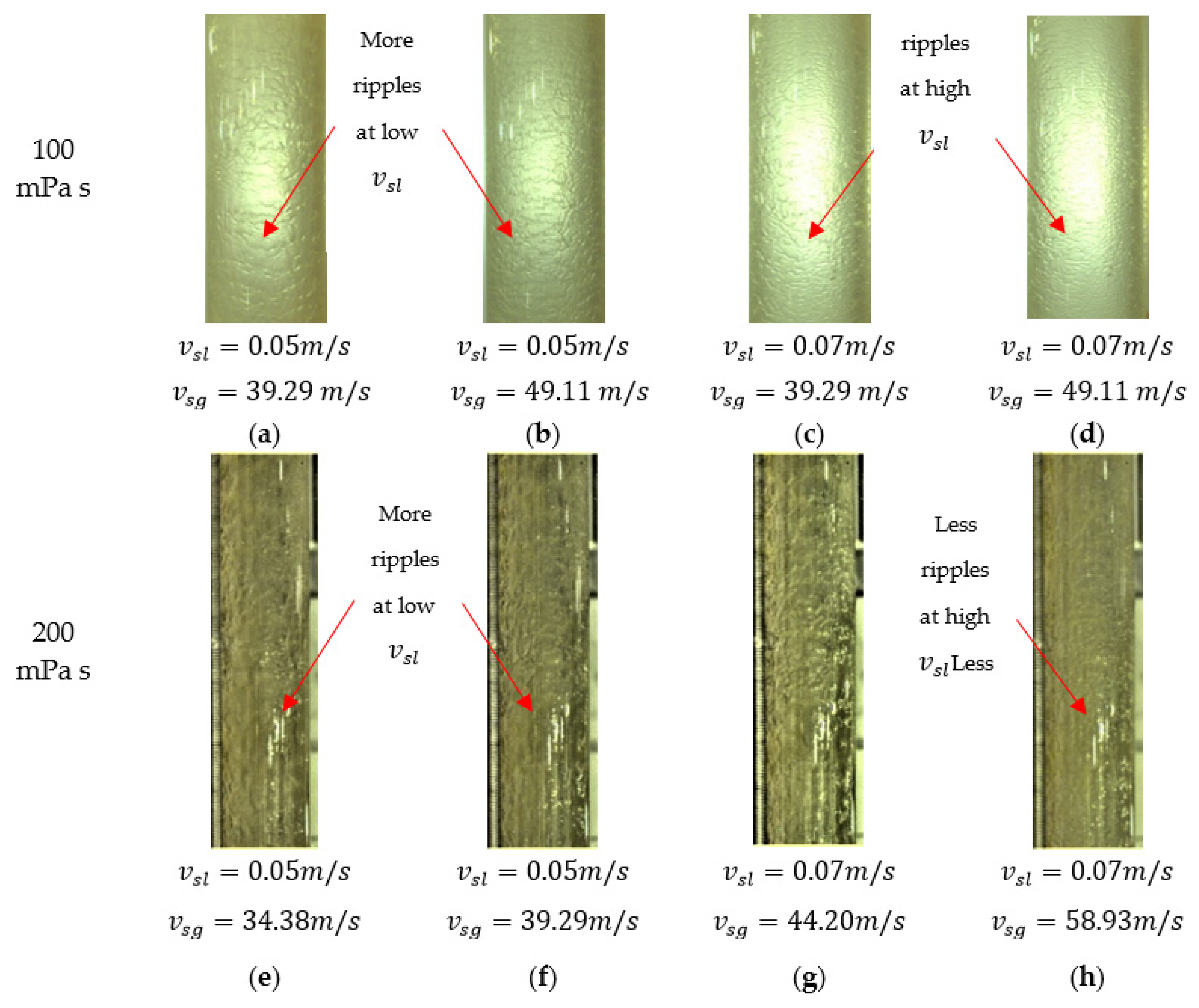
3.1.1. Visual Observations and Identification of Flow Regime

Annular flow was observed at all flow conditions and liquid viscosities under consideration (Figure 4a–h). Downward flow of liquid film was not observed at any flow condition. At all liquid viscosities, the liquid film observed, during experimentation, was relatively thick at low phase velocities. There appeared to be a reduction in thickness of the liquid film when velocity of the gas was increased. The phenomenon persisted even when the velocity of the liquid was increased. The same trend was observed at both viscosities. The velocity of the liquid contributed to the total phase momentum reducing of the thickness of the liquid film. This finding agrees with reports by Fukano and Furukawa [36] who concluded that reduction in the thickness of the liquid film can occur without the influence of liquid viscosity and velocity. Furthermore, it was also observed that, at fixed phase velocities, there is a corresponding increase in liquid film thickness as liquid viscosity increases. In this study, it appeared that the liquid films were thinner at 100 mPa s at all superficial velocities (Figure 4a–d).

In addition, ripples appeared on the liquid film surface at different experimental conditions (Figure 4a–h). The ripples appeared to decrease in roughness when phase velocities were increased. At higher gas velocities in particular, a relatively smoother liquid film surface could be observed. Figure 4 illustrates ripples on the liquid film surface at varied superficial phase velocities for liquid viscosities of 100 and 200 mPa s respectively. At a liquid viscosity of 200 mPa s, for instance, it can be observed that at $v_{sl}$ and $v_{sg}$ values of 0.05 m/s and 34.38 m/s, respectively, the surface of the liquid film is rougher (Figure 4e) compared to the gentle ripples observed at higher superficial gas and liquid velocity of 0.07 m/s and 58.93 m/s, respectively (Figure 4h). Fukano and Furukawa [36] also reported ripples on the surface of the liquid film for the liquid viscosities they employed. They characterized this phenomenon as ripple flow. Furthermore, the visual observations showed that the nature of wavy surfaces differed for varied viscosities even under the same flow conditions. The observed phenomenon agrees with the suggestion by Fukano and Furukawa [36] that interfacial friction factor, which has a direct relationship with wave characteristics, is significantly influenced by liquid viscosity.

3.1.2. Visual Observations and Flow Regime Identification

To clarify the flow patterns identified during the experiments, the flow pattern data obtained was superimposed on the flow pattern maps presented by Shell [25,41] and Taitel et al. [42], respectively (Figure 5).

Created by the Shell Company [25,41] to facilitate the distribution of petroleum products, the flow pattern map presented by Shell employs the superficial gas (abscissa) and liquid Froude (ordinate) number, respectively. The densimetric Froude numbers utilized are defined as follows:

$$F{r}_g=v_{sg}{\left(\frac{{\rho }_g}{\left({\rho }_l-{\rho }_g\right)gD}\right)}^{0.5}, F{r}_l=v_{sl}{\left(\frac{{\rho }_l}{\left({\rho }_l-{\rho }_g\right)gD}\right)}^{0.5}$$

It was observed that the Shell flow pattern map appeared unable to identify and classify data points representing transition to annular flow (Figure 5a). It classified the given data as annular flow. Despite this challenge, the flow pattern map agrees very well with the experimental data. The closeness of the phase properties (${\rho }_l$ = 860 kg/m³, ${\mu }_g$ = 0.00016 Pa s, and $\sigma$ = 0.03 N/m), utilized for the map development, to the experimental fluid properties could account for the observation. Furthermore, adoption of a large diameter (500 mm) for the flow pattern development does not seem to pose any serious limitations.

The flow pattern map developed by Taitel et al. [42] utilizes transition criteria for different flow patterns obtained by analytically developing relationships to calculate the force balance existing between the drag forces and gravity. Predictions of the flow regime map agreed with the experimental data.

3.2. Liquid Holdup

At all liquid viscosities, liquid holdup was observed to decrease as superficial gas velocity increased (Figure 6a). Sharp reductions in liquid holdup were observed when superficial gas velocity was low and became asymptotic when superficial gas velocity was increased above 40 m/s for all liquid viscosities.

Again, it appeared that liquid holdup decreased as superficial liquid velocity increased. However, the observed reductions appeared less significant, particularly at higher liquid viscosities. The observation can be attributed to a lack of impetus of the liquid quantity and velocity to reverse the effects generated by the high gas velocity.

In addition, the results suggest that increasing liquid viscosity increases liquid holdup superficial gas velocities being fixed. Increments in liquid viscosity generates a corresponding increase in shear stresses resulting in greater liquid buildup [1]. The phenomenon is also attributable to decreased liquid entrainment as liquid viscosity increases [1].

3.3. Pressure Drop

Increased pressure drop was observed when superficial gas velocity increased (Figure 6b). This phenomenon can be due to increased friction occurring at the interface between the gas and liquid. Liquid at the interface of the liquid and gas generates comparatively higher interfacial friction than that occurring between the gas and the wall. Higher gas–liquid interface friction occurs when the liquid surface is wavy. Again, increased pressure drop could be because of increased density of the gas phase as a result of liquid entrainment in the gas phase. Finally, when liquid superficial velocity is fixed, an increase in the velocity of the gas generates a corresponding increase in slip and interfacial shear at the gas–liquid interface, ultimately translating into a higher total pressure drop [2].

The influence of superficial liquid velocity on pressure drop was not significant (Figure 6b). This is because, as iterated earlier, it is not possible for the $v_{sl}$values to cause any major changes because they are too small. A closer inspection, when fixed superficial phase velocities are fixed, however, suggests that when the viscosity of the liquid increases there is a corresponding increase in pressure drop. Increased liquid viscosity increases frictional pressure drop during the flow and increases liquid holdup which contributes to increases in the gravitational component of pressure drop. Therefore, total pressure drop will increase when the liquid viscosity is increased because the frictional and gravitational components will correspondingly increase.

3.4. Liquid Film Thickness

Figure 6c illustrates disparities in the thickness of the liquid film for liquid viscosities 100 mPa s, 150 mPa s, 200 mPa s, respectively, with superficial gas velocity. Further investigation reveals that thickness of the liquid film reduces as superficial gas velocity increases. Again, at all superficial liquid velocities and liquid viscosities, the decrease in the thickness of the liquid film thickness was asymptotic. A rapid reduction was observed at low superficial gas velocities.

The thickness of the liquid film was maximum at a viscosity of 200 mPa s and decreased when the viscosity of liquid was reduced. This can be attributed to the growing resistance to the flow conditions as liquid viscosities become high (reducing liquid droplet entrainment and increasing liquid holdup). The observed behaviour of liquid film thickness when subjected to varied gas velocities agrees with reports by authors who experimented with air and water [24,25,31]. Also, Fukano and Furukawa [36] and Kaji and Azzopardi [43], who experimented with liquids with low viscosity, reported similar findings.

3.5. Influence of Various Interfacial Frication Factors on Predictions of Liquid Film Thickness, Gas Void Fraction and Pressure Gradient

For all flow conditions, the combined momentum equation was solved by integrating different interfacial friction factor correlations and comparing the predicted values for liquid film thickness, gas void fraction and pressure gradient predictions for liquid viscosities of 100 and 200 mPa s with experimental data. The effect of combining the popular liquid friction factor of Blasius with several interfacial friction factors is presented. The Oliemans et al. [8] correlation for liquid entrainment fraction is used for this study.

To solve the combined momentum equation, the MATLAB fsolve function was employed. The function fsolve is a non-linear system solver which resolves problems expressed as:

F(x) = 0

(19)

For x (vector or matrix), where F(x) is a function that returns a vector value. Input values for superficial liquid and gas velocities, liquid viscosity and an initial guess were supplied to the MATLAB programme. For the solution procedure, the Levenberg–Marquardt algorithm was activated. The stopping criteria for iteration was set at a termination tolerance of 1e-6. A solution was considered achieved when the value of the liquid film thickness was positive, and the result of F(x) was very close to zero.

3.5.1. Liquid Film Thickness

A comparison of experimental liquid film thickness and predictions of the two-fluid model using the selected correlations of interfacial friction factor at liquid viscosity of 100 and 200 mPa, respectively, as well as $v_{sl}$ of 0.05 m/s and 0.07 m/s, respectively, is shown in Figure 7.

At liquid viscosity of 100 mPa s and $v_{sl}$ values of 0.05 m/s (Figure 7a) and 0.07 m/s (Figure 7b), predictions of the two-fluid model using all $f_i$ correlations exhibit the trend of the experimental data. At $v_{sl}$ of 0.07 m/s, however, it appears that predictions of liquid film thickness agree more with the experimental data at low superficial gas velocities. At both $v_{sl}$and $v_{sg}$ values, the correlations present satisfactory results. The correlations of Belt et al. [32], Ambrosini et al. [30], Wongwises and Kongkiatwanitch [24] and Akagawa et al. [25] present the best performances at both $v_{sl}$ values, respectively.

When the liquid viscosity is increased to 200 mPa s (Figure 7c,d), all predictions by the model underpredict the data at all $v_{sl}$ values. At $v_{sl}$ of 0.05 m/s, the closest predictions are presented (in order of reducing accuracy) by Akagawa et al. [25], Fore et al. [33], Holt et al. [34], Wongwises and Kongkiatwanitch [24] and Ambrosini et al. [30] (Figure 7c). When $v_{sl}$ is increased to 0.07 m/s, the closest predictions are presented (in order of reducing accuracy) by Fore et al. [33], Holt et al. [34], Akagawa et al. [25], Wongwises and Kongkiatwanitch [24] and Ambrosini et al. [30]. It can be concluded that there is better agreement at liquid viscosity of 100 mPa s than at higher viscosity of 200 mPa s.

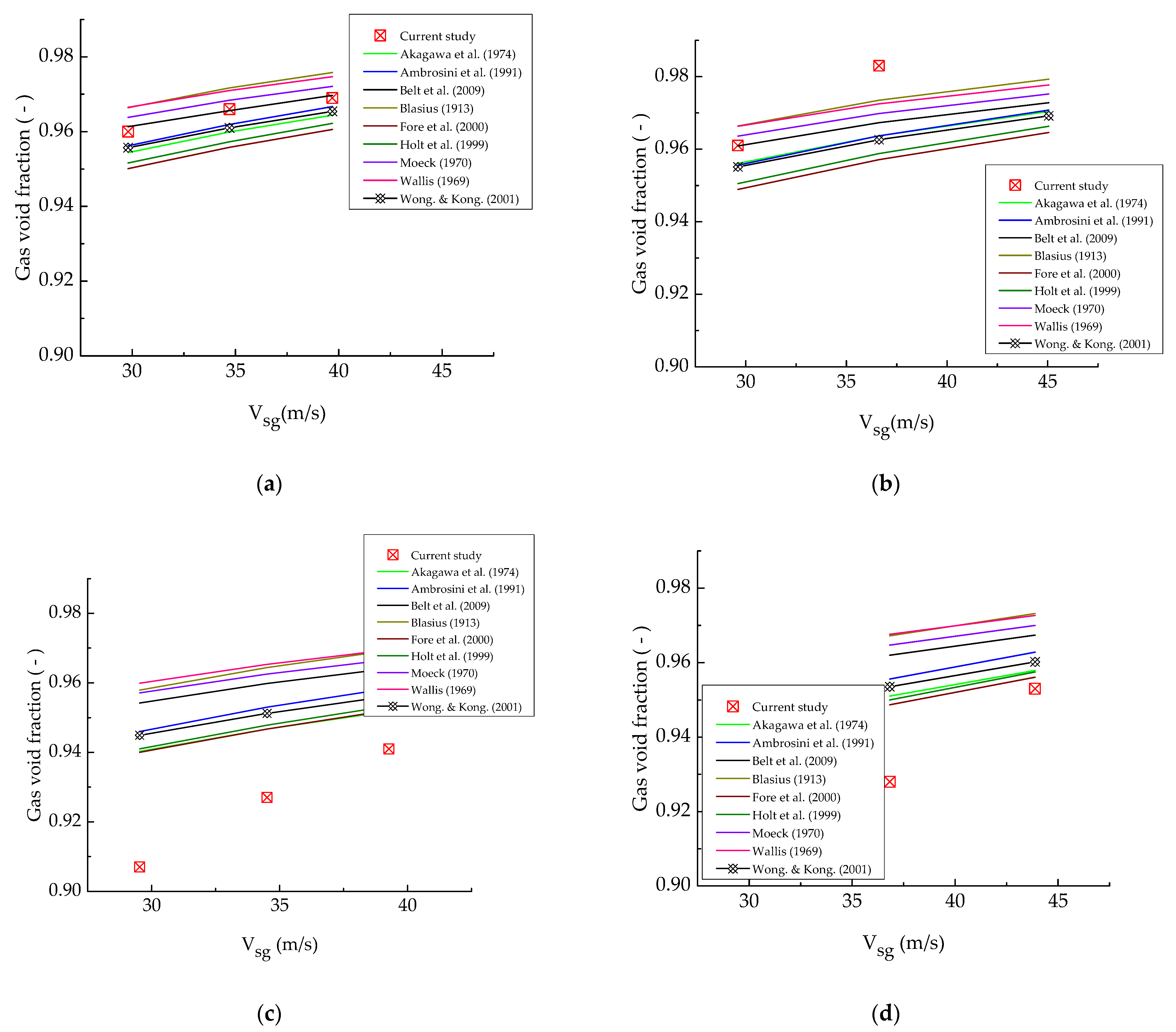
3.5.2. Gas Void Fraction

Figure 8a,b show a comparison of the experimental gas void fraction with the predictions of the two-fluid model at a liquid viscosity of 100 mPa s and $v_{sl}$ values of 0.05 and 0.07 m/s, respectively. At $v_{sl}$ of 0.05 m/s, the predicted gas void fraction values are comparatively accurate for all $f_i$ correlations utilized. At $v_{sl}$ value of 0.07 m/s, predictions agree better at low values of $v_{sg}$ than at high $v_{sg}$ values. For the case of the liquid viscosity at 200 mPa s, reasonable over-prediction of gas void fraction (GVF) values is observed at both $v_{sl}$ values of 0.05 and 0.07 m/s, respectively. Predictions, at both superficial liquid velocities, improve at higher GVF values.

Equation (16) explains the observed characteristics of the predictions in Figure 8 and Figure 9. The equation expresses the mathematical relationship showing that void fraction as a function of superficial gas and liquid velocities as well as accurate predictions of both liquid entrainment fraction and liquid film thickness. In this study, accurate predictions of liquid film thickness become paramount because the other variables can be assumed to be held constant at the specified flow condition. From the equation, it can be inferred that overprediction of liquid film thickness results in underprediction of values of gas void fraction and vice versa. Significant overprediction is observed in Figure 9a as a result of underprediction in liquid film entrainment (Figure 8a).

3.5.3. Pressure Gradient

Figure 9 shows the efficiency of pressure gradient predictions from the selected correlations for interfacial friction factor for liquid viscosities of 100 and 200 mPa s, respectively. The statistical tools, absolute average percent error (AAPE) and average percent error (APE) expressed in Equations (20) and (21) were employed to determine the prediction errors.

$$\mathrm{AAPE}=\frac{1}{n}{\displaystyle {{\displaystyle \sum }}_{i=1}^n}\left|\frac{A_i-F_i}{A_i}\right|$$

(20)

$$\mathrm{APE}=\frac{100\%}{n}{\displaystyle {{\displaystyle \sum }}_{i=1}^n}\frac{A_i-F_i}{A_i}$$

(21)

$n$, $A_i$ and $F_i$ represent the number of times the summation iteration occurs, actual values and predicted values, respectively.

At a liquid viscosity of 100 mPa s (Figure 9a,b), it can be observed that the $f_i$ correlations of both Blasius and Wallis follow the trend of the experimental data but also overpredict the experimental data compared to the correlations. At superficial liquid velocities of 0.05 and 0.07 m/s, predictions of the two-fluid model using the other $f_i$ correlations are satisfactory. Over the entire data for liquid viscosity of 100 mPa s, the four best pressure gradient predictions are achieved using $f_i$ correlations of Belt et al. [32] (AAPE = 23.49, APE = −1.55), Akagawa et al. [25] (AAPE = 28.17, APE = 26.43), Ambrosini et al. [30] (AAPE = 28.02, APE = 26.52), and, Wongwises and Kongkiatwanitch [24] (AAPE = 31.88, APE = 31.88) listed in order of decreasing accuracy, offer the best pressure gradient predictions.

When the liquid viscosity is increased two-fold (Figure 9c,d), the pressure gradient predictions obtained using the selected correlations follow the pattern of the experimental data. At $v_{sl}$ of 0.05 m/s, the $f_i$ correlations of Moeck [35], Wallis [26], Blasius [25] and Fore et al. [33] are observed to give the most accurate predictions. Although the others underpredict the experimental data, their predictions are found to be equally satisfactory. At $v_{sl}$ of 0.07 m/s, the $f_i$ correlations of Wallis [26] and Blasius are observed to slightly overpredict the experimental data. It appears that utilization of the Wongwises and Kongkiatwanitch [24] correlation enables the two-fluid model to predict the trend of the data more accurately than the others.

Statistical analyses, using AAPE and APE, indicate that the $f_i$ correlations of Moeck [35] (AAPE = 25.11, APE = 14.61) offer the best predictions over the data obtained with liquid viscosity of 200 mPa s followed by that of Wallis [26] (AAPE = 28.59, APE = −4.73) and Belt et al. [32] (AAPE = 30.61, APE = 30.14), respectively.

Accurate prediction of pressure gradient requires accuracy in the prediction of geometrical parameters as well as the respective velocities of the liquid film and gas core, all of which rely heavily on accurate predictions of the liquid film thickness. As observed in Figure 7, all the correlations appear to predict the gas void fraction fairly accurately. Furthermore, if liquid friction factor and liquid entrainment fraction are assumed fixed for each flow condition, the pressure gradient predictions of the two-fluid model can be viewed as a direct result of the differences in the approach or theory as well as experimental conditions used for $f_i$ correlation development.

4. Conclusions

An experimental investigation of vertical air and oil (with viscosities ranging between 100 and 200 mPa s) flow in a 0.060 m ID pipe is reported. Superficial air and oil velocity ranges are from 22.37 to 59.60 m/s and 0.05 to 0.16 m/s, respectively. The annular flow pattern at the flow conditions was considered.

A two-fluid model was developed for prediction of gas void, liquid holdup, and pressure gradient. A combined momentum equation for the gas and liquid phases was developed and solved to generate values of liquid film thickness and, subsequently, predict the liquid holdup and pressure gradient at given experimental conditions.

The influence of accuracy of estimation of the interfacial friction factor on accurate determination of the flow characteristics mentioned was investigated by utilizing nine selected correlations. It was observed that although the correlations were developed with low viscosity liquids, the correlations generally present satisfactory performances. For the liquid viscosity of 100 mPa s, the fi correlation of Belt et al. [32] presents the best performance for the prediction of pressure gradient while the correlation of Moeck [35] presents the best prediction at the liquid viscosity of 200 mPa s. The performance of the Belt et al. [32] equation can possibly be attributed to agreement of the flow conditions with their proposed theory that sand-grain roughness of the liquid film is proportional to wave height. The performance of the Moeck [35] correlation could be attributable to the application of viscosity ratios to accommodate the viscosity differences adequately.

Overall, the results indicate that the two-fluid model is a reliable model capable of predicting accurately upward annular flow characteristics involving high-viscosity liquids including liquid film thickness, gas void fraction and pressure gradient in conduits.

References

1. Al-Ruhaimani, F.; Pereyra, E.; Sarica, C.; Al-Safran, E.M.; Torres, C.F. Experimental Analysis and Model Evaluation of High-Liquid-Viscosity Two-Phase Upward Vertical Pipe Flow. SPE J. 2017, 22, 712–735. [Google Scholar] [CrossRef]
2. Alamu, M.B. Investigation of Periodic Structures in Gas-Liquid Flow. Ph.D. Thesis, University of Nottingham, Nottingham, UK, 2010. [Google Scholar]
3. Hamad, F.A.; Faraji, F.; Santim, C.G.S.; Basha, N.; Ali, Z. Investigation of pressure drop in horizontal pipes with different diameters. Int. J. Multiph. Flow 2017, 91, 120–129. [Google Scholar] [CrossRef] [Green Version]
4. Ribeiro, J.X.F.; Liao, R.; Aliyu, A.M.; Liu, Z. Upward interfacial friction factor in gas and high-viscosity liquid flows in vertical pipes. Chem. Eng. Commun. 2019, 1–30. [Google Scholar] [CrossRef]
5. Funahashi, H.; Kirkland, V.K.; Hayashi, K.; Hosokawa, S.; Tomiyama, A. Interfacial and wall friction factors of swirling annular flow in a vertical pipe. Nucl. Eng. Des. 2018, 330, 97–105. [Google Scholar] [CrossRef]
6. Bbosa, B.; DelleCase, E.; Volk, M.; Ozbayoglu, E. A comprehensive deposition velocity model for slurry transport in horizontal pipelines. J. Pet. Explor. Prod. Technol. 2017, 7, 303–310. [Google Scholar] [CrossRef] [Green Version]
7. Alves, I.M.; Caetano, E.F.; Minami, K.; Shoham, O. Modeling Annular Flow Behavior for Gas Wells. SPE Prod. Eng. 1991, 6, 435–440. [Google Scholar] [CrossRef]
8. Oliemans, R.V.A.; Pots, B.F.M.; Trompé, N. Modelling of annular dispersed two-phase flow in vertical pipes. Int. J. Multiph. Flow 1986, 12, 711–732. [Google Scholar] [CrossRef]
9. Vieira, R.E.; Parsi, M.; McLaury, B.S.; Shirazi, S.A.; Torres, C.F.; Schleicher, E.; Hampel, U. Experimental characterization of vertical gas–liquid pipe flow for annular and liquid loading conditions using dual Wire-Mesh Sensor. Exp. Therm. Fluid Sci. 2015, 64, 81–93. [Google Scholar] [CrossRef]
10. Zhang, H.-Q.; Wang, Q.; Sarica, C.; Brill, J.P. Unified Model for Gas-Liquid Pipe Flow via Slug Dynamics—Part 1: Model Development. J. Energy Resour. Technol. 2003, 125, 266–273. [Google Scholar] [CrossRef]
11. Bendiksen, K.H.; Maines, D.; Moe, R.; Nuland, S. The Dynamic Two-Fluid Model OLGA: Theory and Application. SPE Prod. Eng. 1991, 6, 171–180. [Google Scholar] [CrossRef]
12. Aziz, K.; Govier, G.W. Pressure Drop In Wells Producing Oil And Gas. J. Can. Pet. Technol. 1972, 11, 38–48. [Google Scholar] [CrossRef]
13. Hagedorn, A.; Brown, K. The Effect of Liquid Viscosity in Two-Phase Vertical Flow. J. Pet. Technol. 1964, 16, 203–210. [Google Scholar] [CrossRef]
14. Duns, H.; Ros, N.C.J. Vertical flow of gas and liquid mixtures in wells. In Proceedings of the 6th World Petroleum Congress, Frankfurt am Main, Germany, 19–26 June 1963; pp. 451–465. [Google Scholar]
15. Mukherjee, H.; Brill, J.P. Pressure Drop Correlations for Inclined Two-Phase Flow. J. Energy Resour. Technol. 1985, 107, 549–554. [Google Scholar] [CrossRef]
16. Beggs, D.H.; Brill, J.P. A Study of Two-Phase Flow in Inclined Pipes. J. Pet. Technol. 1973, 25, 607–617. [Google Scholar] [CrossRef]
17. Orkiszewski, J. Predicting Two-Phase Pressure Drops in Vertical Pipe. J. Pet. Technol. 1967, 19, 829–838. [Google Scholar] [CrossRef]
18. Fontalvo, E.M.G.; Branco, R.L.C.; Carneiro, J.N.E.; Nieckele, A.O. Assessment of closure relations on the numerical predictions of vertical annular flows with the two-fluid model. Int. J. Multiph. Flow 2020, 126. [Google Scholar] [CrossRef]
19. Sanderse, B.; Buist, J.F.H.; Henkes, R.A.W.M. A novel pressure-free two-fluid model for one-dimensional incompressible multiphase flow. J. Comput. Phys. 2021, 426, 109919. [Google Scholar] [CrossRef]
20. Liu, Z.; Su, Y.; Lu, M.; Zheng, Z.; Liao, R. Frictional Pressure Drop and Liquid Holdup of Churn Flow in Vertical Pipes with Different Viscosities. Geofluids 2021. [Google Scholar] [CrossRef]
21. Imam, M.M.; Basha, M.; Shaahid, S.M.; Ahmad, A.; Al-Hadhrami, L.M. Effect of viscosity on the pressure gradient in 4-inch pipe. ASME Int. Mech. Eng. Congr. Exp. Proc. 2014, 7. [Google Scholar] [CrossRef]
22. Ganat, T.; Ridha, S.; Hairir, M.; Arisa, J.; Gholami, R. Experimental investigation of high-viscosity oil–water flow in vertical pipes: Flow patterns and pressure gradient. J. Pet. Explor. Prod. Technol. 2019, 9, 2911–2918. [Google Scholar] [CrossRef] [Green Version]
23. McNeil, D.A.; Stuart, A.D. The effects of a highly viscous liquid phase on vertically upward two-phase flow in a pipe. Int. J. Multiph. Flow 2003, 29, 1523–1549. [Google Scholar] [CrossRef]
24. Wongwises, S.; Kongkiatwanitch, W. Interfacial friction factor in vertical upward gas-liquid annular two-phase flow. Int. Commun. Heat Mass Transf. 2001, 28, 323–336. [Google Scholar] [CrossRef]
25. Aliyu, A.M.; Baba, Y.D.; Lao, L.; Yeung, H.; Kim, K.C. Interfacial friction in upward annular gas–liquid two-phase flow in pipes. Exp. Therm. Fluid Sci. 2017, 84, 90–109. [Google Scholar] [CrossRef]
26. Wallis, G.B. One-Dimensional Two-phase Flow; McGraw Hill: New York, NY, USA, 1969. [Google Scholar]
27. Sawant, P.; Ishii, M.; Mori, M. Prediction of amount of entrained droplets in vertical annular two-phase flow. Int. J. Heat Fluid Flow 2009, 30, 715–728. [Google Scholar] [CrossRef]
28. Aliyu, A.M.; Almabrok, A.A.; Baba, Y.D. Prediction of entrained droplet fraction in co-current annular gas–liquid flow in vertical pipes. Exp. Therm. Fluid Sci. 2017, 85, 287–304. [Google Scholar] [CrossRef] [Green Version]
29. Zhang, H.-Q.; Wang, Q.; Sarica, C.; Brill, J.P. Unified Model for Gas-Liquid Pipe Flow via Slug Dynamics—Part 2: Model Validation. J. Energy Resour. Technol. 2003, 125, 274. [Google Scholar] [CrossRef]
30. Ambrosini, W.; Andreussi, P.; Azzopardi, B.J. A physically based correlation for drop size in annular flow. Int. J. Multiph. Flow 1991, 17, 497–507. [Google Scholar] [CrossRef]
31. Matsuyama, F.; Sadatomi, M.; Nakashima, K.; Johno, Y.; Shigematsu, T. Effects of surface tension on liquid film behavior and interfacial shear stress in upward annular flows in a vertical pipe. J. Mech. Eng. Autom. 2013, 7, 1–8. [Google Scholar] [CrossRef]
32. Belt, R.J.; Van’t Westende, J.M.C.; Portela, L.M. Prediction of the interfacial shear-stress in vertical annular flow. Int. J. Multiph. Flow 2009, 35, 689–697. [Google Scholar] [CrossRef]
33. Fore, L.B.; Beus, S.G.; Bauer, R.C. Interfacial friction in gas-liquid annular flow: Analogies to full and transition roughness. Int. J. Multiph. Flow 2000, 26, 1755–1769. [Google Scholar] [CrossRef] [Green Version]
34. Holt, A.J.; Azzopardi, B.J.; Biddulph, M.W. Calculation of two-phase pressure drop for vertical upflow in narrow passages by means of a flow pattern specific model. Chem. Eng. Res. Des. 1999, 1, 7–15. [Google Scholar] [CrossRef]
35. Moeck, E.O. Annular-Dispersed Two-Phase Flow and Critical Heat Flux. 1970. Available online: https://astee-tsm.fr/10.1051/tsm/201201037 (accessed on 1 June 2021).
36. Fukano, T.; Furukawa, T. Prediction of the Effect of Liquid Viscosity on Interfacial Shear Stress and Frictional Pressure Drop in Vertical Upward Gas Liquid Annular Flow. Int. J. Multiph. Flow 1998, 24, 587–603. [Google Scholar] [CrossRef]
37. Asali, J.C.; Hanratty, T.J.; Andreussi, P. Interfacial drag and film height for vertical annular flow. AIChE J. 1985, 31, 895–902. [Google Scholar] [CrossRef]
38. Zangana, M.H.S. Film Behaviour of Vertical Gas-Liquid Flow in a Large Diameter Pipe. Ph.D. Thesis, University of Nottingham, Nottingham, UK, 2011. [Google Scholar]
39. Van der Meulen, G.P. Churn-Annular Gas-Liquid Flows in Large Diameter Vertical Pipes. Ph.D. Thesis, University of Nottingham, Nottingham, UK, 2012. [Google Scholar]
40. Shearer, C.J.; Nedderman, R.M. Pressure gradient and liquid film thickness in co-current upwards flow of gas/liquid mixtures: Application to film-cooler design. Chem. Eng. Sci. 1965, 20, 671–683. [Google Scholar] [CrossRef]
41. Pinto del Corral, N. Analysis of Two-Phase Flow Pattern Maps. 2014. Available online: http://www.energetickeforum.cz/ext/2pf/maps/Documents/Analysis_of_maps.pdf (accessed on 1 June 2021).
42. Taitel, Y.; Bornea, D.; Dukler, A.E. Modelling flow pattern transitions for steady upward gas-liquid flow in vertical tubes. AIChE J. 1980, 26, 345–354. [Google Scholar] [CrossRef]
43. Kaji, R.; Azzopardi, B.J. The effect of pipe diameter on the structure of gas/liquid flow in vertical pipes. Int. J. Multiph. Flow 2010, 36, 303–313. [Google Scholar] [CrossRef]
Figure 1. An illustration of the control volume for the momentum balance in Equation (14). (Adapted from Wongwises and Kongkiatwanitch, [24]; and Aliyu et al., [25]).
Energies 14 03485 g001
Figure 2. Experimental setup—(a): experimental rig in vertical position (photo); (b): schematic representation of rig; (c) dimensions of test section. (Adopted from Ribeiro et al., [4], with permission from Taylor and Francis).
Energies 14 03485 g002aEnergies 14 03485 g002b
Figure 3. Variation of oil viscosity with temperature.
Energies 14 03485 g003
Figure 4. Flow patterns observed at different v s g values for v s l values of 0.05 and 0.07 m/s for liquid viscosities of (ad) 100 and (eh) 200 mPa s respectively (Adopted from Ribeiro et al., [33] with permission from Taylor and Francis).
Energies 14 03485 g004
Figure 5. Experimental data super-imposed on the flow pattern maps of: (a) Shell Company [25,41] and (b) Taitel et al. [42] (Adopted from Ribeiro et al., [33]).
Energies 14 03485 g005
Figure 6. Experimental data showing variation of (a) liquid holdup, (b) pressure gradient and (c) thickness of the liquid film with superficial gas velocity for liquid viscosities of 100 mPa s, 150 mPa s and 200 mPa s, respectively, at different v s l values. (Adopted from Ribeiro et al., [33]).
Energies 14 03485 g006
Figure 7. Comparison of experimental liquid film thickness with predictions of two-fluid model using selected f i correlations at 100 (a,b) and 200 (c,d) mPa s.
Energies 14 03485 g007
Figure 8. Comparison of experimental gas void fraction with predictions of two-fluid model using selected f i correlation at 100 (a,b) and 200 (c,d) mPa s.
Energies 14 03485 g008
Figure 9. Pressure gradient predictions using selected fi correlations at 100 (a,b) and 200 (c,d) mPa s.
Energies 14 03485 g009