Deep-Reinforcement-Learning-Based Two-Timescale Voltage Control for Distribution Systems

Abstract

Because of the high penetration of renewable energies and the installation of new control devices, modern distribution networks are faced with voltage regulation challenges. Recently, the rapid development of artificial intelligence technology has introduced new solutions for optimal control problems with high dimensions and dynamics. In this paper, a deep reinforcement learning method is proposed to solve the two-timescale optimal voltage control problem. All control variables are assigned to different agents, and discrete variables are solved by a deep Q network (DQN) agent while the continuous variables are solved by a deep deterministic policy gradient (DDPG) agent. All agents are trained simultaneously with specially designed reward aiming at minimizing long-term average voltage deviation. Case study is executed on a modified IEEE-123 bus system, and the results demonstrate that the proposed algorithm has similar or even better performance than the model-based optimal control scheme and has high computational efficiency and competitive potential for online application.

1. Introduction

1.1. Background and Motivation

The high penetration of distributed generation (DG) energy sources, such as photovoltaic (PV), has made distribution networks faced with the problem of voltage regulation. Usually, the voltage profiles in distribution networks are regulated by the control of slow regulation devices (e.g., on-load tap changers (OLTCs) and shunt capacitors) and fast regulation devices (e.g., PV inverters and static var compensators (SVCs)). While these regulators are all applied to adjust the distribution of reactive power in the grid, the real power flow can also impact the nodal voltages in distribution networks [1,2]. Thus, the real and reactive power control of different devices should be taken into account in order to mitigate possible voltage violations.

The lack of measurement systems (e.g., supervisory control and data acquisition (SCADA) and phasor measurement units (PMUs)) in traditional distribution networks leads to the insufficient measurement of network information, and voltage control methods generally adopt model-based regulation, which rely highly on the precise physical model. In essence, voltage control through real and reactive power optimization is a highly nonlinear programming problem with abundant variables and massive constraints. Solving such problems using mathematical programming methods (e.g., the second-order cone relaxation technique [3] and duality theory [4]) is often limited by the number of variables, and may even fail when the scale of the distribution network is too large. Therefore, heuristic algorithms which are less dependent on the model are applied to solve these problems (e.g., particle swarm optimization (PSO) [5] and genetic algorithm (GA) [6]). However, these algorithms have the shortcomings of high randomness and long search time, and easily fall into local optimal solutions, and as a result cannot meet the requirement of real-time voltage control in a fast time scale. In addition, in these mathematical programming methods and heuristic algorithms, each optimization solution is independent of each other, and if the actual operating condition (e.g., DG outputs) changes slightly, the previous optimization results are often unable to be made full use of in order to achieve a rapid solution.

Recently, artificial intelligence (AI) technology has developed rapidly and been successfully applied in different fields. Therefore, many scholars are interested in exploring its application in power systems. Among AI technology, as a branch of reinforcement learning (RL) theory, DRL employs the “trial and error” mechanism to interact with the dynamic environment to find the optimal policy for the agent [7]. It has great advantages for solving complex multivariable problems, and has already been employed in various power system optimization problems, such as, electricity market planning [8], multi-agent equilibrium games [9], battery energy arbitrage [10], and scheduling the charging of electric vehicles [11].

The expansion of the coverage of SCADA and PMU [12], as well as the construction of internet of things technologies, has provided an effective way for the advanced applications of voltage control based on data-driven and model-free methods. For example, the authors in [13] employ Q-learning to solve a reactive power optimization problem with the discrete control variables being the transformer tap ratio and shunt capacitor. However, the Q-learning method easily falls into the curse of dimensionality since it applies a table to store the corresponding action-value function, and it is only suitable for the problems where the action space and state space are both discrete. Inspired by the strong exploration capacity of neural networks (NNs) towards high-dimensional searching space, deep Q network (DQN) employs an NN to approximate the action-value function to deal with continuous state domains. In [14], a DQN is used to control shunt capacitors. In [15], a double DQN is applied to achieve the optimal control of thermostatically controlled loads (TCLs) to provide voltage-control-based ancillary services. In [16], a multi-agent DQN-based algorithm is put forward to control switchable capacitors, voltage regulators, and smart inverters, where the continuous variables of voltage regulators and smart inverters are discretized. Further, to deal with the problems with continuous state and action space, deep deterministic policy gradient (DDPG) is put forward, where two NNs are used to approximate the policy function and action-value function. In [17], DDPG is applied to learn the control policy of generators in order to regulate all bus voltages into a predefined safe zone. In [18], a voltage-sensitivity-based DDPG method is proposed to realize the local control of PV inverters, and with a specifically designed reward, the goal of minimizing the network power loss and ensuring safe operation in the grid can be achieved. In [19], a novel adaptive volt-var control algorithm based on DDPG is proposed to realize the real-time control of smart inverters in reactive power management. However, the existing voltage control methods using DRL only focus on the reactive power control, and cannot deal with the discrete and continuous control variables simultaneously.

1.2. Novelty and Contribution

To overcome the above limitations, a DRL method combining a DQN method with DDPG is proposed in this paper to deal with discrete and continuous control variables simultaneously. In this method, the discrete variables are resolved based on a DQN agent and the continuous variables are resolved based on a DDPG agent. Considering the response time and control cost of different equipment, a two-timescale voltage control problem is put forward, where the capacitor configuration is decided in the long timescale and the outputs of PV inverters and energy storage batteries are adjusted in the short timescale. The problem is further turned into the Markov decision process (MDP) and solved by the proposed DRL method. A reward is specially designed to achieve the goal of minimizing the long-term average voltage deviation. Both the DQN agent and DDPG agent share the same environment (i.e., the distribution network), and are trained by their interaction with the environment.

The contributions of this article are outlined as follows.

(1)

Multiple types of control equipment including capacitors, energy storage batteries, and PV inverters are considered, and a two-timescale voltage control problem is formulated in order to take the control requirements of these devices into account.

(2)

The control variables are assigned to different agents according to their properties, and these agents share the same environment and are trained simultaneously.

(3)

A DRL method is proposed to solve the optimal voltage control problem, where the discrete variables are solved using a DQN agent and the continuous variables are solved using a DDPG agent, and this method can realize real-time control.

2. Voltage Problem Formulation

In this section, the two-timescale voltage control problem is formulated, where the control devices, including capacitors, batteries, and PV inverters, are considered.

2.1. System Description

In this voltage control problem, the real power regulation is achieved by adjusting the charging/discharging power of batteries, and the reactive power regulation is realized by adjusting the on/off states of capacitors and the outputs of PV inverters. Taking the response time and control cost of different devices into account, the total control process can be divided into long timescale control and short timescale control. Specifically, the entire time period can be divided into N_T intervals, and each interval can be further divided into N_t slots. In the long timescale, the capacitors’ configurations are made at the beginning of each interval T, and in the short timescale the outputs of PV inverters and batteries are adjusted at the beginning of each slot t.

(1)

Capacitor modeling

During each T, the reactive power supported by the capacitor installed at bus i, Q_Cap,i(T, t), can be expressed as a function of binary control variable a_cap,i(T)∈{0,1}, which indicates the off/on status of the capacitor; that is,

$$Q_{Cap,i}\left(T,t\right)=a_{cap,i}\left(T\right)\cdot Q_{Cap,i}^{rated},$$

(1)

where $Q_{Cap,i}^{reted}$ is the rated reactive power of the capacitor. When a_cap,i(T) = 1, the capacitor is connected to the grid and the reactive power provided by it is $Q_{Cap,I}^{reted}$; when a_cap,i(T) = 0, the capacitor is disconnected from the grid.

(2)

Battery modeling

During every t, the state variable (state of charge) of the battery installed at bus i is denoted as SOC_i(T, t), which is subject to the upper and lower boundaries [20]; that is,

$$SO{C}_{i,\min }\le SO{C}_i\left(T,t\right)\le SO{C}_{i,\max }$$

(2)

The charging/discharging power of the battery, P_batt,i(T, t), can be expressed as

$$P_{Batt,i}\left(T,t\right)=a_{batt,i}\left(T,t\right)\cdot P_{Batt,i}^{max}$$

(3)

$$-1\le a_{batt,i}\left(T,t\right)\le 1$$

(4)

where a_batt,i(T, t) is the control variable and when a_batt,i(T, t) is positive, the battery is charging. When a_batt,i(T, t) is negative, the battery is discharging. The new state of charge after taking the control action can be represented as

$$SO{C}_i\left(T,t+1\right)=SO{C}_i\left(T,t\right)+P_{Batt,i}\left(T,t\right).$$

(5)

(3)

PV inverter modeling

Suppose all PV units in the grid are equipped with a smart inverter. On every t, the active power provided by the PV unit installed at bus i is known as P_PV,i(T, t) and its apparent power rating is $S_{PVi}^{rated}$. Then, the reactive power provided by the smart inverter, Q_PV,i(T, t), can be expressed as

$$Q_{PV,i}\left(T,t\right)=a_{pv,i}\left(T,t\right)\cdot {\overline{Q}}_{PV,i}\left(T,t\right)$$

(6)

$${\overline{Q}}_{PV,i}\left(T,t\right)=\sqrt{{\left(S_{PV,i}^{rated}\right)}^2-{\left(P_{PV,i}\left(T,t\right)\right)}^2}$$

(7)

$$-1\le a_{pv,i}\left(T,t\right)\le 1$$

(8)

where a_pv,i(T, t) is the control variable of the PV inverter.

2.2. Two-Timescale Voltage Control Model Formulation

In this paper, a radial distribution network with N+1 buses is considered, where Bus 0 is the root, representing the point of common coupling. The voltage magnitude, active power, and reactive power are all converted to per unit (p.u.). The objective of the voltage control problem is to minimize the long-term average voltage deviation by configuring the on/off status of capacitors on every interval T in the long timescale and adjusting the charging/discharging power of batteries and the outputs of PV inverters on every t in the short timescale. Then, the two-timescale voltage control problem based on power flow equations can be formulated as follows:

$$\underset{\begin{array}{c}\left\{a_{cap}\left(T\right)\right\}\\ \left\{a_{batt}\left(T,t\right),a_{pv}\left(T,t\right)\right\}\end{array}}{\min }\mathbb{E}\left[{\displaystyle \sum _{T=1}^{\infty }{\displaystyle \sum _{t=1}^{N_t}{\displaystyle \sum _{i=1}^N{\left(U_i\left(T,t\right)-1\right)}^2}}}\right]$$

(9)

s.t.

$$\left(1\right)–\left(3\right)$$

(10)

$${\displaystyle \sum _{i\in \mathbf{\psi }\left(j\right)}\left[P_{ij}\left(T,t\right)-I_{ij}^2\left(T,t\right)r_{ij}\right]-P_j\left(T,t\right)}={\displaystyle \sum _{k\in \mathbf{\varphi }\left(j\right)}{P}_{jk}\left(T,t\right)}$$

(11)

$${\displaystyle \sum _{i\in \mathbf{\psi }\left(j\right)}\left[Q_{ij}\left(T,t\right)-I_{ij}^2\left(T,t\right)r_{ij}\right]-Q_j\left(T,t\right)}={\displaystyle \sum _{k\in \mathbf{\varphi }\left(j\right)}{Q}_{jk}\left(T,t\right)}$$

(12)

$$U_j^2\left(T,t\right)=U_i^2\left(T,t\right)+\left(r_{ij}^2+x_{ij}^2\right)I_{ij}^2\left(T,t\right)-2\left(r_{ij}{P}_{ij}\left(T,t\right)+x_{ij}{Q}_{ij}\left(T,t\right)\right)$$

(13)

$$I_{ij}^2\left(T,t\right)=\left(P_{ij}^2\left(T,t\right)+Q_{ij}^2\left(T,t\right)\right)/U_i^2$$

(14)

$$P_j\left(T,t\right)=P_{L,j}\left(T,t\right)+P_{Batt,j}\left(T,t\right)-P_{PV,j}\left(T,t\right)$$

(15)

$$Q_j\left(T,t\right)=Q_{L,j}\left(T,t\right)-Q_{Cap,j}\left(T,t\right)-Q_{PV,j}\left(T,t\right)$$

(16)

where U_j(T, t) is the voltage magnitude of bus j; I_ij(T, t) is the current amplitude of segment (i, j); r_ij and x_ij are the resistance and reactance of segment (i, j), respectively; P_ij(T, t) and Q_ij(T, t) are the active and reactive power flowing from bus i to bus j, respectively; ψ(j) is the parent bus set of bus j, where the power flows from the parent bus to bus j; and ϕ(j) is the child bus set of bus j, where the power flows from bus j to the child bus.

It can be observed that the optimization problem (9) involves many control variables, including the continuous variables of batteries and PV inverters and the discrete variables of capacitors, which makes problem (9) non-convex and generally NP-hard. When the grid is large and thus involves many control variables, traditional model-based methods may obtain suboptimal solutions, which will consume more time or even be impossible to solve. Additionally, this is a multi-stage planning problem, where the decisions of each type of controller are not made at the same stage. To overcome these difficulties, a model-free method based on deep reinforcement learning is introduced to solve the problem, which is detailed in Section 3.

3. Deep Reinforcement Learning Solution

In this section, the voltage control problem is first formulated as an MDP, and then a model-free solution based on deep reinforcement learning is put forward, in which the control variables of different controllers are assigned to different agents. The solution of discrete variables is based on a DQN agent while the solution of continuous variables is based on a DDPG agent.

3.1. Markov Decision Process

In order to solve the voltage control problem with DRL algorithms, the optimal configurations of different controllers have to be modeled as an MDP. An MDP is defined by the tuple (S, A, P, R, γ), and it is used to describe the interaction process between the agents (i.e., different controllers) and the environment (i.e., the power flow of distribution systems). In this paper, for each agent, the state space S is continuous while the action space A is either discrete or continuous. P, usually unknown, is the state transition probability indicating the probability density of the next state s_t+12∈S under the current state s_t and action a_t. R is the reward on each transition, which is denoted as r_t =R(s_t, a_t), and γ∈[0, 1] is the discount factor. Then, the goal of the voltage control problem is to solve the MDP—that is, to learn the optimal policy of each agent to maximize the reward, which is associated with the long-term average voltage deviation.

In DRL algorithms, the policy μ, expressed as μ(a|s), is a mapping function of the action a_t taken by the agent in the state s_t. During the training process, the action-value function, also called the Q-function, represents the expected discounted reward after taking action a in the state s with policy μ, and can be denoted as $Q_{\mu }\left(\mathit{s},\mathit{a}\right)={\mathbb{E}}_{\mu }\left[{\displaystyle {\sum }_{k=0}^{T_{all}}{\gamma }^k{r}_k}|{\mathit{s}}_0=\mathit{s},{\mathit{a}}_0=\mathit{a}\right]$, where T_all is the episode length. Using the Bellman equation, the Q-function can be further expressed as $Q_{\mu }\left({\mathit{s}}_t,{\mathit{a}}_t\right)={\mathbb{E}}_{\mu }\left[r_t+\gamma Q_{\mu }\left({\mathit{s}}_{t+1},{\mathit{a}}_{t+1}\right)|{\mathit{s}}_t,{\mathit{a}}_t\right]$. Then, solving the optimal policy μ^* is equivalent to solving the optimal Q-function, that is, $Q_{\mu }{}^{*}=\underset{\mu }{\max }{Q}_{\mu }\left(\mathit{s},\mathit{a}\right)$.

3.2. DQN-Based Agent for Discrete Variables

The configurations of the capacitors are made at the beginning of each interval T. For the discrete variables of capacitors, a DQN—a value-based DRL method—is introduced to handle the control problem with continuous state space and discrete action space.

The classic DQN method, based on the Q-learning method, uses a deep neural network (DNN) to estimate the continuous Q-function, and the DNN can be indicated as a Q network, that is, Q_μ(s, a; θ_Q), whose input is the state vector and output is the Q-values for all possible actions. The experience replay buffer D is used to store experiences e_T = (s_T, a_T, r_T, s_T+1), and a mini batch is applied to store M randomly sampled experiences. In order to update the parameters of the Q network, a target Q network is employed with the parameters of ${\mathbf{\theta }}_Q^{\prime }$. Then, using stochastic gradient descent (SGD), the parameters of the Q network can be updated based on the mini batch and the loss function, which can be expressed as

$$L\left({\mathbf{\theta }}_Q\right)=\underset{i\in M}{\mathbb{E}}\left[{\left(r_i+\gamma \underset{a\prime }{\max }{Q}_{\mu }\left({\mathit{s}}_{i+1},\mathit{a}\prime ;{\mathbf{\theta }}_Q^{\prime }\right)-Q_{\mu }\left({\mathit{s}}_i,{\mathit{a}}_i;{\mathbf{\theta }}_Q\right)\right)}^2\right],$$

(17)

where the parameters of the target Q network ${\mathbf{\theta }}_Q^{\prime }$ are updated by copying the parameters of the Q network θ_Q periodically for every B.

For the capacitor agent, the state consists of the average positive power of each bus during the interval T and the action during the last interval T-1, that is, ${\mathit{s}}_{cap}\left(T\right)={\left[{\overline{\mathit{P}}}^T\left(T\right),{\mathit{a}}_{cap}^T\left(T-1\right)\right]}^T$. The action a_cap(T) = [a_cap,1(T),…,a_cap,Ncap(T)]^T is defined as the configurations of capacitors, where a_cap,i(T)∈{0, 1} and N_cap is the number of capacitors. When the state s_cap(T) is fed into the input layer and passes through the hidden layers, the output layer generates the Q-values of the particular configurations of all capacitors with a total number of 2^Ncap neurons. Then, the action having the maximum Q-value is selected for the next interval. To meet the control object, the reward is designed as the negative of the voltage deviation of all buses, which can be expressed as $r_{cap}\left(T\right)=-{\displaystyle \sum _{t=1}^{N_t}{\displaystyle \sum _{i=1}^N{\left(U_i\left(T,t\right)-1\right)}^2}}$.

In order to ensure that the agent can both explore the unknown environment and make use of the knowledge it has already grasped, the ε-greedy strategy is employed to select action; that is,

$${\mathit{a}}_T=\left\{\begin{array}{cc}random \mathit{A}\hfill & \hfill \beta <\epsilon \\ \underset{a_T\in A}{\arg \max }{Q}_{\mu }({\mathit{s}}_T,{\mathit{a}}_T;{\mathbf{\theta }}_{\mathit{Q}})\hfill & \hfill \beta \ge \epsilon \end{array}\right.$$

(18)

where ε∈[0, 1] and is a constant, and β∈[0, 1] and is randomly generated by computer. When β < ε, the agent randomly selects an action in the action space; otherwise, the agent selects the action that has the maximum Q-value in the current state.

The capacitors’ configuration based on the DQN is depicted in Figure 1. During the training period, the agent selects actions based on (18), while during the execution process, based on the current state, the agent selects the action that has the maximum Q-value.

3.3. DDPG-Based Agent for Continuous Variables

Based on the configuration of capacitors in the intervals, the outputs of PV inverters and batteries are adjusted at the beginning of each slot t. For the continuous control variables of PV inverters and batteries, DDPG is applied to deal with the control problem with continuous state space and continuous action space.

The DDPG method not only employs a DNN to simulate the Q-function, but also uses a DNN to estimate the policy function. It adopts a typical actor–critic framework, which realizes the policy action and action evaluation by designing the actor network μ(s; θ_μ) and critic network Q_μ(s, a; θ_Q), respectively. Like the DQN, the target actor network μ’(s, θ_μ’) and target critic network Q’_μ’(s, a; θ_Q’) are also applied.

During the training process, the continuous action is decided based on the following function:

$${\mathit{a}}_t=\mu \left({\mathit{s}}_t;{\mathbf{\theta }}_{\mu }\right)+{\xi }_t$$

(19)

where ξ_t is the noise used to randomly search actions in the action space. Experience replay buffer and mini batch are also employed. Then, the critic network can be updated by minimizing the loss function as in (17); that is,

$$L\left({\mathbf{\theta }}_Q\right)=\underset{i\in M}{\mathbb{E}}{\left[y_i-Q_{\mu }\left({\mathit{s}}_i,{\mathit{a}}_i;{\mathbf{\theta }}_Q\right)\right]}^2$$

(20)

$$y_i=r_i+\gamma Q_{\mu }^{\prime }\left({\mathit{s}}_{i+1},{\mu }^{\prime }\left({\mathit{s}}_{i+1};{\mathbf{\theta }}_{\mu \prime }\right);{\mathbf{\theta }}_{Q\prime }\right).$$

(21)

The actor network can be updated using the policy gradient, which can be expressed as

$${\nabla }_{{\mathbf{\theta }}_{\mu }}\mu =\underset{i\in M}{\mathbb{E}}\left[{\nabla }_{a}Q\left({\mathit{s}}_i,{\mathit{a}}_i;{\mathbf{\theta }}_Q\right)\cdot {\nabla }_{{\mathbf{\theta }}_{\mu }}\mu \left({\mathit{s}}_i;{\mathbf{\theta }}_{\mu }\right)\right].$$

(22)

Then, the target networks are soft-updated as follows:

$${\mathbf{\theta }}_Q^{\prime }=\lambda {\mathbf{\theta }}_Q+\left(1-\lambda \right){\mathbf{\theta }}_Q^{\prime }$$

(23)

$${\mathbf{\theta }}_{\mu }^{\prime }=\lambda {\mathbf{\theta }}_{\mu }+\left(1-\lambda \right){\mathbf{\theta }}_{\mu }^{\prime },$$

(24)

where the parameter λ≪1.

For the PV inverters and batteries agent, the state consists of the voltage amplitude of all buses and the state of charge of batteries at time t, that is, s_PVbatt(t) = [U^T(t), SOC^T(t)]^T. The action includes the action variables of PV inverters and batteries, that is, a_PVbatt(t) = [${\mathit{a}}_{PV}^T$(t), ${\mathit{a}}_{batt}^T$(t)]^T, ${\mathit{a}}_{PV}\left(t\right)={\left[a_{PV,1}\left(t\right),\dots ,a_{PV,N_{PV}}\left(t\right)\right]}^T$, and ${\mathit{a}}_{batt}\left(t\right)={\left[a_{batt,1}\left(t\right),\dots ,a_{batt,N_{batt}}\left(t\right)\right]}^T$, where N_PV and N_batt are the number of PV inverters and batteries, respectively, and a_PV,i(t)∈[−1, 1] and a_batt,i(t)∈[−1, 1]. The reward is designed similarly to that of the capacitors agent, which can be denoted as $r_{PVbatt}\left(t\right)=-{\displaystyle \sum _{i=1}^N{\left(U_i\left(t\right)-1\right)}^2}$.

Furthermore, the action implementation method of forced constraint output is adopted in order to take the capacity boundaries of batteries into account—that is, when SOC_i(t + 1) = SOC_i(t) + a_PV,i(t)∙$P_{batt,i}^{max}$ is outside of the upper and lower boundaries, only the amount of chargeable (dischargeable) power SOC_i.max-SOC_i(t) (SOC_i(t)-SOC_i.min) is charged (discharged).

The control of PV inverters and batteries based on DDPG is demonstrated in Figure 2. During the training period, the state s_PVbatt(t) is fed into the actor network and an action a_PVbatt(t) is generated based on (19). Then, the state and action enter the critic network and the corresponding Q-value is generated. During the execution period, with well-trained networks, the agent chooses its action based on the state, that is, a_PVbatt(t) = μ(s_PVbatt(t); θ_μ).

3.4. Algorithm and Computation Process

The two-timescale voltage control for distribution systems based on DRL is demonstrated in Algorithm 1.

Algorithm 1 Two-timescale voltage control scheme for distribution systems based on DRL.

1: For the capacitors agent based on DQN, initialize the parameters θQ,DQN randomly; initialize the target Q network with ${\mathbf{\theta }}_{Q,DQN}^{\prime }$ = θQ,DQN; initialize replay buffer DDQN

2: For the PV inverters and batteries agent based on DDPG, initialize the actor and critic networks with θμ,DDPG and θQ,DDPG; initialize target actor and critic network with θμ’,DDPG =θμ,DDPG, θQ’,DDPG =θQ,DDPG; initialize replay buffer DDDPG

3: Initialize capacitors agent state sDQN1

4: for T = 1 to NT do

5:  Get the action acapT from (18)

6:  Execute acapT in the power flow environment and get the initiation state of DDPG agent: sPVbattT1

7:  for t = 1 to Nt do

8:   Get the action  aPVbattTt from (19); execute aPVbattTt in the power flow environment and get the reward rPVbattTt and new state s’PVbattTt

9:   Store the experience in the replay buffer DDDPG

10:  Sample a random mini batch from DDDPG and update the actor and critic networks using (20), (21) and (22).

11:  Soft update the target actor and critic networks using (23) and (24)

12: end for

13: Get the reward of capacitors rcapT; get the new state s’capT

14: Store the experience in the replay buffer DDQN

15: Sample a mini batch randomly from DDQN and update the Q network for DQN

16: if mod(T,B) = =0 then

17:  Update the target Q network for DQN: ${\mathbf{\theta }}_{Q,DQN}^{\prime }$=θQ,DQN

18: end if

19:end for

4. Numerical Study

In this section, the implementation details of the proposed two-timescale voltage control scheme based on DRL are described.

4.1. Simulation Setup

A modified IEEE 123-bus distribution test system was applied to carry out the numerical tests. Based on the original 123-bus multi-phase unbalanced network [21], the system was changed into a balanced system and the numbering of each node was reorganized as shown in Figure 3. Twelve PV units with smart inverters were installed at 12 buses, and their capacities and locations are listed in

Table 1. The capacities and locations of 12 installed PV units.

PV Location	PV Capacity	PV Location	PV Capacity	PV Location	PV Capacity
24	300 kW	63	300 kW	92	400 kW
31	300 kW	70	400 kW	100	400 kW
39	200 kW	79	400 kW	106	300 kW
50	400 kW	87	200 kW	113	200 kW

. Four capacitors were installed in the grid at buses 20, 59, 66, and 114, each with a capacity of 40 kvar. Four energy storage batteries were installed at buses 56, 83, 96, and 116, each with a maximum capacity of 600 kWh and rated charge/discharge power of 100 kW. The load power was modified from the real data of an area in Jiangsu province, China (i.e., on each bus, the peak load value was set to the sum of the loads on three phases in the original 123-bus distribution network, and the load curve after standardization was the same as that after the standardization of the real load of an area in Jiangsu province, China). Thus, the load value of each bus was equal to the load curve multiplied by its peak load. All parameters in this distribution system were converted to a consistent base, where the base voltage was 4.16 kV and the base power was 100 MVA.

In the theory of DRL, the parameters that define the architecture of the NNs are of great importance, and the selection of architecture depends on the actual application scenario. For example, convolutional neural networks (CNNs) are often used to deal with complex problems in the image domain, whereas recurrent neural networks (RNNs) are often used to process sequence data. For the voltage control problem raised in this paper, a fully connected NN was sufficient for the task at hand. Based on [22], the number of hidden layers was chosen to be 2 and the number of neurons in each hidden layer was first selected according to that in the upper layer and the lower layer. Then, the model was trained, the output was checked to see if there was overfitting, and the parameters were adjusted until a satisfactory output was obtained. According to the above system setting, the four capacitors generated 2⁴ = 16 combinations of discrete actions, and the PV inverters and batteries produced 16 continuous actions. For the DQN agent, the Q network consisted of three fully connected layers: one input layer, two hidden layers with 95 and 22 neurons, respectively, and one output layer with 16 neurons. The sigmoid function was used at the end of the output layer to keep the Q-value within [0, 1]. For the DDPG agent, the actor and critic networks were also composed of three fully connected layers, with hidden layers of 90, 30 units, and 46, 14 units, respectively. The output layer of the actor network consisted of 16 neurons and the output layer of the critic network had 1 neuron. The tanh function was applied at the end of the actor network to keep the action variables within [−1, 1]. All the hidden layers used rectified linear unit (ReLU) as the activation function. The detailed settings of other hyper-parameters are declared in

Table 2. Settings of other DRL parameters.

Item	Value
Replay buffer size for DQN agent	50
Mini-batch size for DQN agent	8
Target Q network updating cycle	10
Learning rate for DQN network	0.01
Replay buffer size for DDPG agent	1000
Mini-batch size for DDPG agent	64
Learning rate for critic network	0.001
Learning rate for actor network	0.001
Discount factor	0.99
Soft-updating parameter λ	0.005

. Optimal power flow was employed as the environment for these DRL agents. The proposed algorithm was run in Python using the Pytorch framework, and the training process was executed on CPU.

4.2. Case Study

In this subsection, we evaluate the performance of the proposed DRL scheme using the modified IEEE 123-bus system. A total of 2880 data points, comprising load data and PV outputs, were used as training data, as demonstrated in Figure 4. Meanwhile, another 288 data points were used as test data, as depicted in Figure 5.

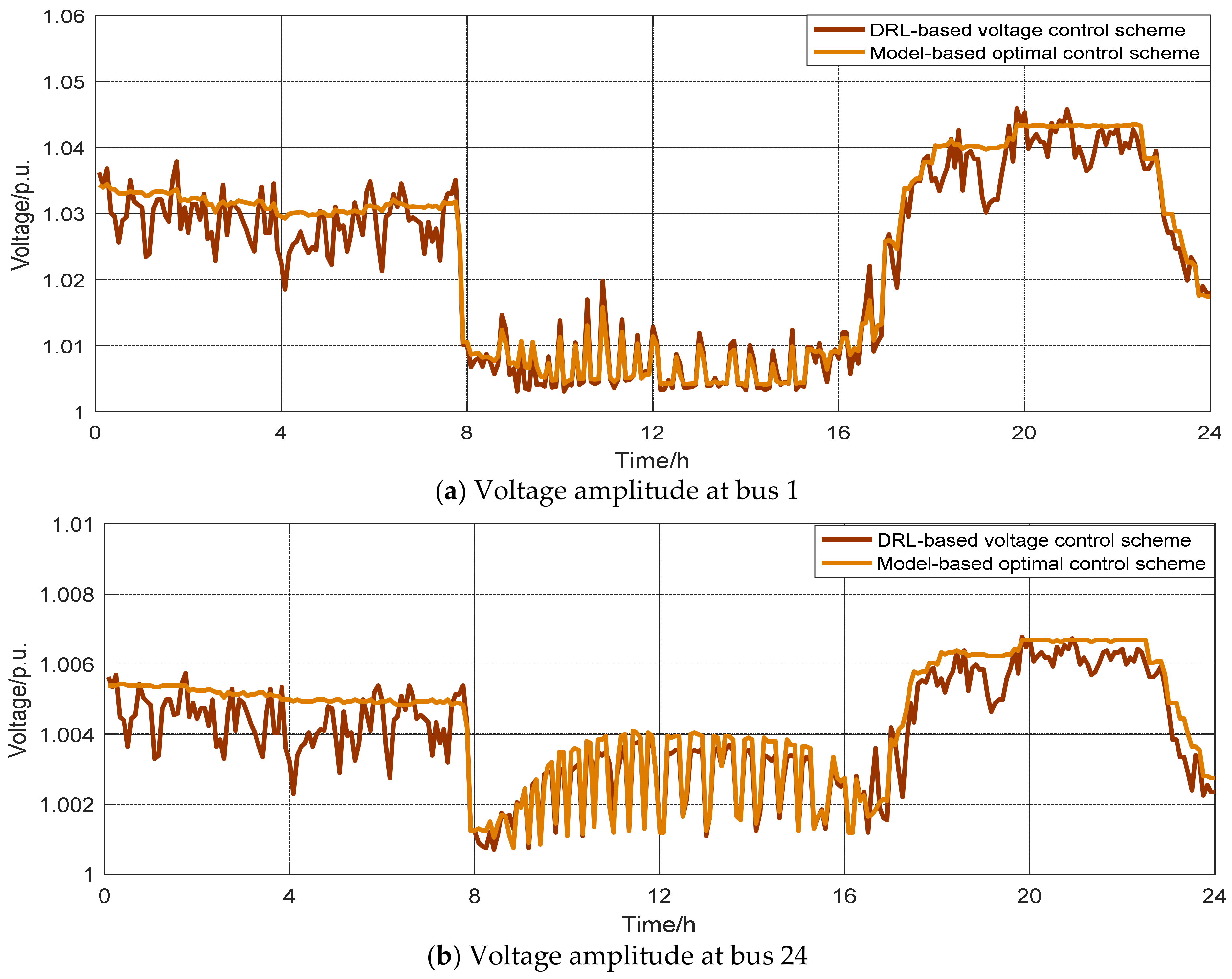
First, based on the optimal power flow, the voltage distribution of this grid without any voltage control was analyzed. In this paper, the interval T was defined as 30 min and the slot t was assumed to be 5 min. The PV outputs were based on the clear day in Figure 5. The buses experiencing voltage issues were bus 1, bus 2, bus 7, and bus 123, which violated the maximum voltage limit of 1.05. Take for example the voltage amplitudes at bus 1 and bus 24 (with PV unit installation), which are depicted by the blue curve in Figure 6.

Then, the learning performance of the proposed DRL method was investigated. Following the procedure shown in Algorithm 1, the DQN and DDPG agents were trained. During the training process, the daily PV generation and load consumption combinations were randomly chosen from the training set, as demonstrated in Figure 4, to represent different grid operation conditions. Training was performed for 300 episodes, and each episode finished after training 288 samples from one day. Figure 7 displays the episode reward values and average rewards in the training period, where the episode reward value is the sum of all the rewards obtained during a given episode and the average reward value is the average of every four episode reward values. It can be observed that in the early stages the reward value was very low because of the limited learning experiences. As the training process continued, the agents gradually evolved and the reward value increased. Later, the reward curves fluctuated due to the random control attempts of both the DQN and DDPG agents to determine the correct policy actions. After about 60 episodes, the reward curve flattened out gradually, indicating the DRL agents’ ability to realize voltage control.

During the test period, the trained DRL agents were employed to control the capacitors, batteries, and PV inverters according to the test data in Figure 5, and the PV outputs were based on the clear day. As demonstrated in Figure 6, compared with the case without voltage control, these trained DRL agents demonstrated an effective performance for voltage control and all bus amplitudes were maintained within the safety limit, especially the buses having voltage issues. Thus, we can conclude that the proposed algorithm enables the controllers to explore the relationship between their configurations and the inherent uncertainty and variability in the PV outputs and load power, and to take corresponding policies when faced with new operating conditions.

4.3. Comparison with the Model-Based Optimal Control Scheme

In order to compare the performance of the proposed DRL method, a model-based optimal control scheme called a two-stage optimal control scheme was applied. The model-based optimal control scheme aims to minimize the daily voltage deviation, and was assumed to have full knowledge of the model and parameters of the distribution network. In this method, the configurations of capacitors, batteries, and PV inverters were decided at the beginning of each interval and the outputs of batteries and PV inverters were further adjusted based on the capacitors configuration at the beginning of each slot.

As demonstrated in Figure 6, in most cases the control effect of the DRL-based method was similar to or even better than that of model-based method, since the model-based method considers the optimal control throughout a day, while the DRL-based method can realize real-time control according to the current state of the power grid.

The execution time of the model-based control method and our proposed DRL-based method targeting all of the day’s 288 samples is demonstrated in

Table 3. Execution time of model-based control method and DRL-based method.

Method	Time (s)
Model-based control method	1107.7629
Our proposed DRL-based control method	0.1964

. It can be seen that the proposed DRL-based method took only 0.1964 s, much less than the 1107.7629 s of the model-based method. Therefore, the proposed algorithm shows high computational efficiency and has competitive potential in online application.

In order to evaluate the dynamic response performance of the proposed DRL-based controller under time-varying PV outputs, the case of a cloudy day was studied. The outputs of the PV units were based on the cloudy day in Figure 5, which show a great deal of fluctuation. The results of the model-based optimal control scheme and the proposed DRL-based voltage control scheme are depicted in Figure 8. It can be seen that the proposed DRL-based controller could respond quickly to the PV fluctuations, which is very important in order to realize the demand of real-time control. Additionally, in the model-based scheme, the controller needs prior knowledge of the PV outputs over a period of time, which is often inaccurate in the case of PV fluctuations. In the proposed DRL-based scheme, the controller adjusts its action based on the current state of the power grid, and is more reliable.

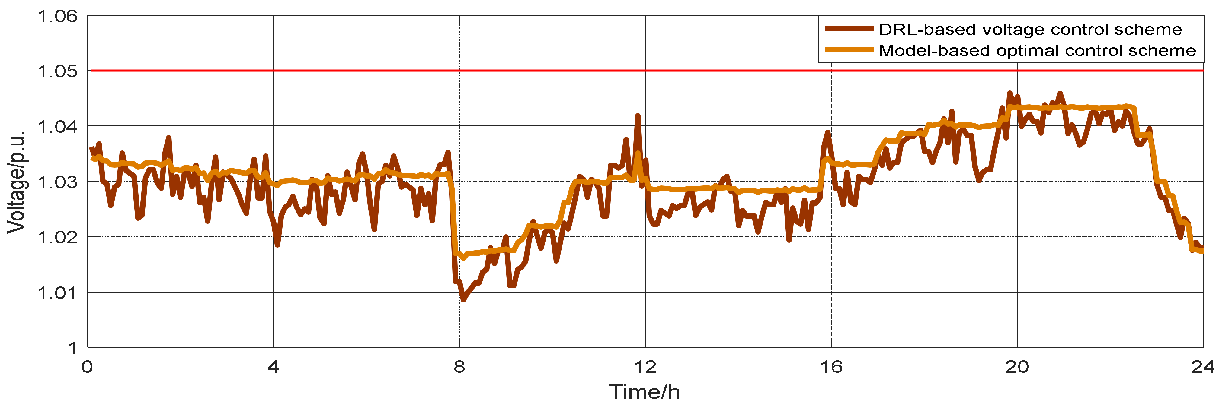
In order to evaluate the control performance of the proposed DRL-based voltage controller under extreme weather conditions, a case study was carried out for a scenario where there were no PV outputs at all. The results of the model-based optimal control scheme and the proposed DRL-based voltage control scheme are demonstrated in Figure 9. The voltage amplitudes of all buses were controlled below 1.05 and it can be seen that the proposed DRL-based controller still had better control performance without PV outputs. From the results of Figure 7, Figure 8 and Figure 9, it can be observed that the trained DRL-based controller worked very well in different scenarios, and could adapt to similar but slightly different data, which verifies the generalization ability of the proposed algorithm.

5. Conclusions

In this paper, a two-timescale voltage control scheme based on a DRL method is proposed to control multiple types of equipment, including capacitors, energy storage batteries, and PV inverters, for optimal voltage control in the distribution network. Control variables are assigned to different agents according to their properties, which share the same environment and are trained simultaneously to cooperate with each other. Specifically, the discrete variables are solved using a DQN agent and the continuous variables are solved using a DDPG agent. A specially designed reward is applied to achieve the goal of minimizing long-term average voltage deviation. Case studies showed that the proposed algorithm had similar or even better performance than the model-based optimal control scheme, and had high computational efficiency, enabling the realization of real-time control. Additionally, the proposed DRL-based controller could adjust its action based on the current state of the power grid. It had better dynamic response performance and could enact a quick response to PV fluctuations. Future work will focus on designing the reward function to achieve more control objectives and take various operating constraints into consideration.

References

- Zhang, L.; Chen, Y.; Shen, C.; Tang, W.; Liang, J. Coordinated voltage regulation of hybrid AC/DC medium voltage distribution networks. J. Mod. Power Syst. Clean Energy 2018, 6, 463–472. [Google Scholar] [CrossRef] [Green Version]
- Hu, X.; Liu, Z.-W.; Wen, G.; Yu, X.; Liu, C. Voltage Control for Distribution Networks via Coordinated Regulation of Active and Reactive Power of DGs. IEEE Trans. Smart Grid 2020, 11, 4017–4031. [Google Scholar] [CrossRef]
- Tang, Z.; Hill, D.J.; Liu, T. Fast Distributed Reactive Power Control for Voltage Regulation in Distribution Networks. IEEE Trans. Power Syst. 2019, 34, 802–805. [Google Scholar] [CrossRef]
- Xie, Y.; Liu, L.; Wu, Q.; Zhou, Q. Robust model predictive control based voltage regulation method for a distribution sys-tem with renewable energy sources and energy storage systems. Int. J. Electr. Power Energy Syst. 2020, 118, 105749. [Google Scholar] [CrossRef]
- Chen, S.; Hu, W.; Chen, Z. Comprehensive Cost Minimization in Distribution Networks Using Segmented-Time Feeder Reconfiguration and Reactive Power Control of Distributed Generators. IEEE Trans. Power Syst. 2016, 31, 983–993. [Google Scholar] [CrossRef]
- Sun, K.M.; Chen, Q.; Zhao, P. Genetic algorithm with mesh check for distribution network topology reconfiguration. Autom. Electr. Power Syst. 2018, 42, 64–71. (In Chinese) [Google Scholar]
- Zhao, H.; Zhao, J.; Qiu, J.; Liang, G.; Dong, Z.Y. Cooperative Wind Farm Control with Deep Reinforcement Learning and Knowledge-Assisted Learning. IEEE Trans. Ind. Inform. 2020, 16, 6912–6921. [Google Scholar] [CrossRef]
- Ye, Y.; Qiu, D.; Li, J.; Strbac, G. Multi-Period and Multi-Spatial Equilibrium Analysis in Imperfect Electricity Markets: A Novel Multi-Agent Deep Reinforcement Learning Approach. IEEE Access 2019, 7, 130515–130529. [Google Scholar] [CrossRef]
- Li, H.Z.; Wang, L.; Lin, D.; Zhang, X.Y. A nash game model of multi-agent participation in renewable energy consumption and the solving method via transfer reinforcement learning. Proc. CSEE 2019, 39, 4135–4149. (In Chinese) [Google Scholar]
- Cao, J.; Harrold, D.; Fan, Z.; Morstyn, T.; Healey, D.; Li, K. Deep Reinforcement Learning-Based Energy Storage Arbitrage with Accurate Lithium-Ion Battery Degradation Model. IEEE Trans. Smart Grid 2020, 11, 4513–4521. [Google Scholar] [CrossRef]
- Li, H.; Wan, Z.; He, H. Constrained EV Charging Scheduling Based on Safe Deep Reinforcement Learning. IEEE Trans. Smart Grid 2019, 11, 2427–2439. [Google Scholar] [CrossRef]
- Hojabri, M.; Dersch, U.; Papaemmanouil, A.; Bosshart, P. A Comprehensive Survey on Phasor Measurement Unit Applications in Distribution Systems. Energies 2019, 12, 4552. [Google Scholar] [CrossRef] [Green Version]
- Shang, X.Y.; Li, M.S.; Ji, T.Y.; Zhang, L.L.; Wu, Q.H. Discrete reactive power optimization considering safety margin by dimensional Q-learning. In Proceedings of the 2015 IEEE Innovative Smart Grid Technologies—Asia (ISGT ASIA), Bangkok, Thailand, 3–6 November 2015; pp. 1–5. [Google Scholar]
- Yang, Q.; Wang, G.; Sadeghi, A.; Giannakis, G.B.; Sun, J. Two-Timescale Voltage Control in Distribution Grids Using Deep Reinforcement Learning. IEEE Trans. Smart Grid 2020, 11, 2313–2323. [Google Scholar] [CrossRef] [Green Version]
- Lukianykhin, O.; Bogodorova, T. Voltage Control-Based Ancillary Service Using Deep Reinforcement Learning. Energies 2021, 14, 2274. [Google Scholar] [CrossRef]
- Zhang, Y.; Wang, X.; Wang, J.; Zhang, Y. Deep Reinforcement Learning Based Volt-VAR Optimization in Smart Distribution Systems. IEEE Trans. Smart Grid 2020, 12, 361–371. [Google Scholar] [CrossRef]
- Duan, J.; Shi, D.; Diao, R.; Li, H.; Wang, Z.; Zhang, B.; Bian, D.; Yi, Z. Deep-Reinforcement-Learning-Based Autonomous Voltage Control for Power Grid Operations. IEEE Trans. Power Syst. 2020, 35, 814–817. [Google Scholar] [CrossRef]
- Sun, X.; Qiu, J. Two-Stage Volt/Var Control in Active Distribution Networks with Multi-Agent Deep Reinforcement Learning Method. IEEE Trans. Smart Grid 2021, 1. [Google Scholar] [CrossRef]
- Beyer, K.; Beckmann, R.; Geißendörfer, S.; von Maydell, K.; Agert, C. Adaptive Online-Learning Volt-Var Control for Smart Inverters Using Deep Reinforcement Learning. Energies 2021, 14, 1991. [Google Scholar] [CrossRef]
- Al-Saffar, M.; Musilek, P. Reinforcement Learning-Based Distributed BESS Management for Mitigating Overvoltage Issues in Systems with High PV Penetration. IEEE Trans. Smart Grid 2020, 11, 2980–2994. [Google Scholar] [CrossRef]
- Kersting, W.H. Radial distribution test feeders. In Proceedings of the IEEE Power Engineering Society Winter Meeting, Columbus, OH, USA, 28 January—1 February 2001; Volume 2, pp. 908–912. [Google Scholar] [CrossRef]
- Heaton, J. Heaton Research the Number of Hidden Layers. 2017. Available online: https://www.heatonresearch.com/2017/06/01/hidden-layers.html (accessed on 9 June 2021).
Figure 1.
The control of capacitors based on the DQN agent.