
Identification of the Determinants of the Effectiveness of On-Road Chicanes in the Village Transition Zones Subject to a 50 km/h Speed Limit


Road and Bridge Department, Faculty of Civil and Environmental Engineering, West Pomeranian University of Technology Szczecin, 71-311 Szczecin, Poland
*
Author to whom correspondence should be addressed.
Energies 2021, 14(13), 4002; https://doi.org/10.3390/en14134002
Submission received: 26 May 2021
/
Revised: 15 June 2021
/
Accepted: 29 June 2021
/
Published: 2 July 2021
(This article belongs to the Special Issue New Perspectives and Challenges in Traffic and Transportation Engineering Supporting Energy Saving in Smart Cities)
Abstract
:In recent years, in which a considerable increase in the road traffic volumes has been witnessed, traffic calming has become one the key issues in the area of road engineering. This concerns, in particular, trunk roads passing through small villages with a population of up to 500 and the road section length within the village limits of ca. 1400–1700 m. A successful traffic calming scheme must involve primarily effective reduction in inbound traffic speed. A review of the data from various countries revealed that chicanes installed in the transition zones may have a determining effect on the success of the traffic calming project. The effectiveness of such chicanes depends mainly on the type of chicane, its location on the carriageway, its shape and the size of the lateral deflection imposed by the chicane on the inbound lane. The purpose of this study was to identify the speed reduction determinants in traffic calming schemes in village transition zones, based on a central island horizontally deflecting one lane of a two-lane two-way road with 50 km/h speed restriction. As part of the study, vehicle speeds were measured just before and after the chicanes under analysis. Furthermore, the inbound lane traffic volumes were measured in field and a number of factors were identified, including the applied traffic management scheme, road parameters, view of the road ahead and of the village skyline, isolated buildings, road infrastructure and adjacent roadside developments. The obtained data were analysed with a method employing tautologies of the selected 32 factors affecting the drivers’ perception. A single aggregate parameter was proposed for assessing the coincidence of the influence of selected factors on speed reduction. The analysis of the existing schemes and the results of statistical analyses carried out in this study confirmed the authors’ hypothesis that the combined selected factors produce a desirable effect and that they should be additionally enhanced by the application of solar powered devices.
Keywords:
traffic calming; transition zone; chicane; speed restriction; speed reduction; solar cells
1. Introduction
An increase in the traffic volumes observed in the recent decades exacerbates transport-related problems in small towns and villages lying on busy through roads. Taking the above into account, in various countries, traffic calming schemes have started to be introduced in design guidelines for both transition zones and for the entire sections of the through roads within the village limits [1,2,3,4]. The ever-increasing volumes of traffic lead, in many cases, to an increase in the number of road traffic incidents [4,5,6,7], higher noise levels [8,9,10,11] and increased concentrations of exhaust fumes and pollutants [4,11,12] along the entire section of the road’s passage through the village. In numerous instances, private plots of the villagers and a high density of buildings do not allow unrestricted expansion of the existing road system [13,14]. All these factors have an adverse effect on the acceptance and perception of the road section passing through the village and on the local residents’ living conditions [15,16,17,18,19]. Rapid accumulation of these factors can be encountered, especially on the relatively short sections of roads carrying traffic through villages (according to data given in the Danish [1], British [2,19,20,21] and Polish design guidelines [22] and in the article on the design requirements for the arterial roads in Iran [23]). In the literature, this problem has been discussed for many years; however, the focus has mainly been on design requirements for roads carrying through traffic in built-up areas [1,2,3,4,13,24] while less attention has been paid, so far, to village transition zones [25,26,27]. The first traffic safety analyses on through roads crossing rural areas were conducted in the 1990s in Denmark [1] and the United Kingdom [2,19,20,23,28] and, later on, also in Canada [18], Germany [3], Sweden [26], Spain [29,30] and in the USA [19,31]. To prevent similar incidents from occurring on many through roads of lesser importance, the introduction of traffic calming schemes has been recommended in many countries, for application both in the transition zones and over the whole length of the road within the built-up area, e.g., in Austria [32], Denmark [1,33], France [34], the United Kingdom [2,35], Germany [3], Italy [36], Iran [37], Poland [13,22], Sweden [26], Spain [29,30], Switzerland [38] and in the USA [31,39,40,41]. These recommendations are confirmed in numerous publications (e.g., Danish [1,10], British [2,4,8,11], Belgian [9], American [12], and Italian [14] ones), in which the authors argue that it is a stochastic process, making the adverse impact of the road on the surrounding environment dependent on the actual traffic speeds. However, considering the regional road classes one should differentiate the impacts of traffic-calming measures on the reduction in speed depending on the speed limit applied on the approach to and within the village limits [42,43,44]. Based on the analyses of available data and the described results of experimental research projects conducted on the completed traffic calming schemes, it has been concluded that the implementation of traffic calming measures and various speed control schemes resulted in reducing the number of road traffic accidents by ca. 40–50% on average (according to [4]—40%, [20]—10–15%, [28]—54%, [32]—45%, [41]—40–50%, [45]—8–71%, [46]—40–50%).
The most frequently used traffic calming measures are based on horizontal or vertical deflection, depending on the speed limit applicable on the road and the main design parameters of the road in question [1,2,4]. Although horizontal deflections (due to use of chicanes) may bring speed reduction without causing discomfort of passing through vertical traffic calming measures, the design guidelines [1,2,3] recommend consideration of many additional aspects in the design process, such as the applied traffic control measures, lighting system, location along the approach section, etc. An important—in the authors’ opinion—problem regarding the location of the chicane in the transition zone to the village has been more extensively described, for example in [42,43,44]. In [3,19,26], it is also stressed that the fundamental problem with using horizontal traffic calming measures, especially in rural areas, is the need to ensure the means of passage for oversized agricultural vehicles. However, the analysis of the above problems presented in German [3,27], Swedish [26], and American [19,21,28,47] publications showed that the suggested resultant speed reduction data obtained mainly from research conducted on test tracks or from simulation research fail to take into account a number of parameters related directly to the adjacent features in the transition zone and that have an unquestionable influence on the drivers’ perception. These problems were addressed in [42,44] in reference to roads with 70 km/h speed limit or in publication [43], analysing the synergy of various traffic calming measures on the passage through a village lying on regional roads with 70 km/h, 50 km/h and 40 km/h speed limit zones. The current state of knowledge on the scale of speed reduction in the transition zones into villages is discussed in various road engineering circles, but it is still advisable to search for methods to describe the synergy of the numerous factors of the road surroundings that have an effect on the drivers’ perception and to obtain more efficient scores of the expected speed reduction. This research area still has a great analytical potential and could be mandatorily implemented in many countries in village transition zones on regional roads.
This article deals with the evaluation of the effectiveness of a specific traffic calming measure, namely a chicane deflecting one lane, installed in the village transition zones on two-lane single carriageway regional roads with the speed limit of 50 km/h posted on the B-33 sign. In this article, the authors implemented the methods and conclusions from article [44] based on the data obtained on roads with 70 km/h speed limit, elaborating on them considerably and supplementing them with new factors observed on roads with a 50 km/h speed limit. The state of knowledge on the scale of speed reduction due to on-road chicanes, against the existing body of scientific research, is presented in Section 2. The relevant test sections and the assumptions adopted in the research conducted on roads with a 50 km/h speed limit are characterised in great detail in Section 3. In Section 4, the authors managed to demonstrate a high consistency between the analysed variables, i.e., between the chosen parameters of speed distribution and the proposed aggregate parameter representing the transition zone surroundings. This allowed them to state in the final conclusions that the proposed method of selecting the type of chicane and its placement in the transition zone to the village should be further developed and researched on other roads, or with other design options of horizontal traffic calming measures.
2. Background
The recommended distances on which speed restriction should be implemented vary between the currently applicable design guidelines and various scientific publications [1,2,3,27]. The lengths of the speed limit zones depend primarily on the hierarchy of the road and on the total length of the road’s passage through the village. The process of designing a traffic calming scheme over the length of the passage of a road through a village is a complex task, involving experimental testing and analytical studies. Different options tend to be chosen in different countries based on the local empirical studies on the drivers’ behaviour and habits, and on the resultant speed restrictions applied in the village approach zones. These options take into account the data on the achieved speed reductions, obtained from studies conducted in test track conditions [19,21,28,47] or speed reductions achieved during research conducted with the use of traffic simulators [12,24], and the results of research projects employing speed radar devices installed on existing roads [14,19,46], but also the results of research on the impact of the existing road lighting systems on drivers’ perception, and on the use of solar technologies in road infrastructure components, conducted in the natural environment [48,49,50,51,52] or in an “artificial” environment with traffic simulators [53,54].
Still, most of the above-mentioned experimental research results refer to “artificial” environments lacking the natural surroundings of the road, with the only variables being class of the road, speed restriction, width of the traffic lane, size of horizontal deflection [1,2,3], and also the location and size of lateral obstructions installed directly on the chicane or on the edge of the bending lane [21,28,47]. The shape of the chicane, its physical length and the length of its influence on drivers, as well as the resultant speed reduction were additionally taken into account in [27,32]. However, a majority of scientific studies refer to horizontal or vertical traffic calming measures situated on a through roads in the central parts of the villages or on suburban streets in larger towns and cities. Studies addressing directly the issue of speed reduction in the village transition zones were carried out in several countries, including Germany [3,27], Austria [32], Italy [14] and the USA [19,55,56,57].
Summing up the above review of the results of the existing research, it can be stated that the variation in the amount of speed reduction is stochastic in nature and the basic qualitative and quantitative description thereof depends on many very diverse factors, as described above. A comparison of the data from the above-mentioned studies demonstrates the presence of fundamental differences between the respective results and numerous deficiencies in repeatability of ∆v results obtained in the respective countries. Considering the above, it is advisable to search for the ways in which many other additional factors acting in combination impact the speed reduction process, to understand it better and thus make it more effective. In the authors’ opinion, the above-mentioned studies lack an analysis of:
- existing traffic control devices (i.e., location of the upright signs related to the built-up area and the view of the village skyline or individual buildings;
- various road parameters and road infrastructure components related to the built-up area, visible or not visible from the driver’s seat on the approach to the village;
- visibility of the road ahead and the village skyline or single buildings situated in the vicinity of the road;
- adjacent roadside development (open rural area, rural area including a tree row or small groves of trees or forest).
The analysis of the conclusions given in [42,44] showed that the design process should also include the aspects associated with the actual features adjacent to the road in the transition zone under analysis, i.e., the existing traffic management scheme, road design parameters, adjacent roadside development and visibility conditions. The research conclusions, due to demonstrated high consistency of the speed reduction data and the speed change index with the aggregated parameter of the combined effect of various factors characterising the road surroundings, as proposed by the authors have, in the author’s opinion, a significant research potential, which can be utilised in subsequent studies. However, publications [42,44] refer to transition zones with a 70 km/h speed limit, in which chicanes horizontally deflecting one lane by 2 m were implemented. Still, no research results are available for road sections with a 50 km/h speed limit and various types of chicanes resulting in different amounts of horizontal deflection. These aspects were considered in the current study.
Figure 1 illustrates the state of knowledge contained in previous publications.
3. Materials and Methods
3.1. Assumption of the Homogeneity of Parameters of the Road Sections under Comparison Adopted in the Research
The main condition for obtaining robust relationships is the homogeneity of most of the factors describing the studied stochastic object. To this end, purposeful sampling [58,59] should be used, which allows to ensure obtaining a homogenous set of data, that is a set of variables of one kind (i.e., binary and qualitative). This approach to statistical analyses allows the researchers to determine the influence of the selected independent variables on one dependent variable. In the studies described above, the factors characterising the independent variables were the factors defining the surroundings of the road in the transition zone, and the dependent variables were the speed distribution parameters. To assess the influence of the road surroundings on the reduction in speed, from nearly 100 analysed transition zones, the authors chose only regional road sections with 50 km/h speed limits (posted on the B-33 sign placed before the transition zone or just before the chicane). All the test sections were lit by lighting systems conventionally used in built-up areas, covering also the surroundings of the chicane or the area behind it.
All the chosen test sections were situated on renewed regional roads with the pavement in a very good condition, with drainage system in proper working order and traffic control devices clearly visible to the motorists. The traffic controls included raised pavement markers (RPM) or light emitting diode systems and solar powered upright signs. The width of the traffic lane on most of the test sections was 3.5 m. Only on two test sections with 2 m horizontal deflection, were the traffic lanes 3 m wide. Hard shoulders were present only on four sections including, a semi-circular island chicane imposing 6 m horizontal deflection.
On most of the test sections, comparable hourly traffic volumes ranging between 200 and 500 veh/h, and similar proportions of heavy vehicle traffic of 3.5–6% were recorded. Only four test sections carried higher traffic volumes in the region of 850 veh/h. The correlation coefficient of speed reduction for the noted hourly traffic volume level in both directions was R = −0.29, and R = −0.18 for the traffic volume level on the inbound lane alone. Taking this into account, the effect of traffic volumes on the extent of the speed reduction noted was ignored in further analyses.
All speed surveys were conducted in summer (June, July and August), on working days from 10:00 a.m. till 4:00 p.m. in sunny weather with dry road surfaces and under good natural lighting conditions.
3.2. Description of the Test Sections
For the purpose of the survey of the actual vehicle speeds on two-lane two-way through roads with a speed limit of 50 km/h posted on the B-33 traffic sign, the authors identified twelve test sections located in village transition zones. The test sections were situated in open rural areas or in rural areas including a row of trees lining the road or small groves in the roadside area. The chicanes affecting one lane only installed on the test sections differ considerably in terms of shape, length and width (Figure 2). On four sections horizontal deflection a = 6 m was applied, on one section a = 2.5 m, on three sections a = 2.15 m, and on two sections a = 2 m. On two sections, selected for comparison purposes, no chicanes were installed. Conventional traffic signs U-5, U-6 and C-9 (Figure 2a) were placed on the chicanes. Tapers on road markings before and after the chicane differed depending on the size of horizontal deflection and on local conditions associated with the presence of road structures or access points to agricultural fields. The taper ratios applied before and after the chicane are represented in Figure 2a. To show the taking of the lane and horizontal deflection of the vehicle paths, HGV envelopes a are presented in Figure 2b, parallel to the chicane layout plans. An in-depth analysis of the HGV envelope (drawn assuming that passage by the chicane kerb will be avoided) demonstrated that with “more aggressive” taper ratios of 1:7 and 1:5, on curved sections of the traffic lane, the vehicle envelope extended beyond the traffic lane, and the path of the outer wheels went beyond the roadway edge into the dirt shoulder. Only with the 1:10 taper and 2.5 m horizontal deflection did the envelope fit completely within the traffic lane width. When the lane was deflected by 6 m and on roads with paved shoulders, both the outer wheels of the tractor-trailer unit and the vehicle body envelope went beyond the traffic lane area into the paved shoulder. An analysis of the vehicle envelopes demonstrated their dependence the configuration of the following factors: shape of the chicane, traffic lane width, amount of horizontal deflection and the applied taper ratio.
Layout of the vertical traffic signs E-17 “entry sign” and D-42 “built-up area” was another important characteristic of the sections under analysis. In accordance with the vertical traffic signs design trends given in the design guidelines [1,2,13] and in publications [25,42], chicanes should be located after the upright sign E-17 placed at the administrative boundary and the built-up area sign D-42. However, in reality, chicanes were located both past these signs and also between them, and on approach to them. Furthermore, in a few cases of villages sprawling over very large areas with dispersed settlement patterns, they were not accompanied by these signs at all.
All the test sections were located in rural areas. Seven of them were situated in an open area, five of them run through an area overgrown with small groves of trees or tree rows lining the road. The test sections differed significantly in terms of: chicane parameters and factors related to traffic management scheme, road design parameters, adjacent roadside development in the transition zone and visibility conditions.
3.3. Adopted Measurement Methodology
The process of assessment of the effectiveness of chicanes located in the village transition zones with a 50 km/h speed limit, the same as on regional road sections with 70 km/h speed limit, started with an analysis of the vehicle speeds measured before and after the chicane. The measurement apparatus for simultaneous measurement of the traffic volume and vehicle speeds in both directions of traffic [60] was used, as was the case in the study reported in [44]. The measurements covered both traffic lanes in all cases. Using the prescribed measuring procedures that make it possible to immediately assess the number of free-flow vehicles, the surveys were stopped when the number of free-flow vehicles on the inbound lane exceeded 100. The speed survey duration was 2–3 h on average. Speed measurements were correlated one with another and they were conducted simultaneously at points located before and after the chicane, thus making it possible to determine the actual speed reductions achieved for the respective vehicles. The test stations were always located at the same distance from the taper end to avoiding measuring vehicle speeds on curves. As the apparatus can distinguish free-flow situations in either direction of traffic, values needed for the purpose of the performed analysis could be selected on completion of the survey. As mentioned before (in Section 3.1), only small differences in hourly traffic volumes were found on the sections under analysis, and the differences in the speed distribution parameters between free-flow and stable-flow situations were also small as a consequence. Taking this into account, only free-flow values were analysed in the further part hereof.
3.4. Selection of Appropriate Statistical Tests
Analysing the effect of various factors on the traffic speed and the extent of the reduction in the speed, the authors performed a number of statistical tests and adopted the conventional statistical inference methodology. In addition to the significance test, goodness-of-fit test and the test for homogeneity, i.e., the standard tests, the measured speeds were subjected also to nonparametric tests, i.e., the test of independence and the median test. Standard statistical tests used for speed results served, in the first instance, to verify whether the speed populations had normal distributions. The Kolmogorov and Pearson goodness-of-fit tests were used for this purpose. Considering that the speed populations have, as a rule, a continuous probability distribution, more reliable results were obtained in the Kolmogorov goodness-of-fit test. The Pearson goodness-of-fit test depends on variance tests results and, in the cases under analysis, the results of the tests of variance varied, hence the use of the Pearson goodness-of-fit test was considered questionable. Based on the test results, it was assumed that all the populations with a continuous distribution had a normal distribution.
Another Kolmogorov–Smirnov goodness-of-fit test was carried out in relation to the “before” and “after” speed populations to examine whether these populations vary in any way.
Since on a number of test sections a small difference in speeds ∆v = vbefore − vafter was noted and the results of Kolmogorov–Smirnov goodness-of-fit tests varied, nonparametric tests were considered in further analyses. Similarly to the statistical inference methodology described in articles [42,44], the nonparametric tests allowed the authors to determine whether two analysed features (not necessarily measurable ones) were independent, i.e., whether the speed distributions depended on the test station location. The nonparametric tests (of independence and median) were also carried out for the successive sections ordered by the amount of reduction in the speed measured after the chicane. In both tests, positive results were obtained on most of the test sections, confirming the relevance of the test station location, meaning that a change in speed took place across the treatment.
3.5. Main Assumptions Taken in the Qualitative Analysis Concerning Determination of the Speed Reduction Determinants
The estimated speed range data for all the test sections are given in Figure 3. On two sections, No. 11 and No. 12, with no chicanes in place, test stations were located before and after the road sign communicating the boundary of the village (E-17) and the built-up area (D-42). Taking into consideration the fact that traffic calming schemes are implemented in the transition zones primarily to achieve reduction in the village entry speed, Figure 3 shows also the value of v85after (85th percentile speed after the chicane).
Since different types of the chicanes were analysed, Figure 3 also shows symbolic representations of the chicanes, the amount of horizontal deflection a and the l/2a ratio, taking into account the relationships given in the Austrian guidelines [32]. The shape of the chicane is related directly to its length and the length-to-width ratio, since, according to the conclusions from the research results published in [27,32], these parameters were critical to the extent of speed reduction ∆v85. However, the data in Figure 3 show that, in the analysed case, neither the lateral deflection of the traffic lane a, nor the l/2a above-mentioned ratio was a factor critical to the extent of speed reduction and, what is more, no relationship of these factors with the vehicle speed was confirmed. The analysis of the estimated speed ranges data (Figure 3) showed a considerable variation in the speed values, which is independent of the shape of the chicanes, amount of lateral shift and speed reduction. Therefore, the coefficients of correlation of ∆v85 and ∆vav speed reductions related to the amount of the horizontal shift of traffic lane a and the l/2a ratio were compared in Table 1.
The speed variations were particularly scattered on sections No. 2, No. 5 and No. 11. What is more, this dispersion is distinctive both before and after the chicane. When analysing the results of similar studies described in articles [42,44], the authors examined the conditions on the approach and through the treatment to find the cause of the demonstrated changes in the dispersion of speeds. Given the conclusions concerning the effect the adjacent roadside development and the visibility conditions have on traffic speed reduction and inbound speed to the village, visualisations of the relevant conditions on the approach and across the treatment on section No. 2 are presented in Figure 4. The visualisations presented below were developed on the basis of the resultant drivers’ field of focal attention and based on the conclusions from earlier studies on drivers’ central and peripheral vision field, as described in publications [16,18,61].
An analysis of the conditions on the approach and through the treatment shown in Figure 4a demonstrates that the adjacent roadside development on the approach to the chicane with various speeds fails to communicate the built-up area to drivers. They can see only the B-33 signs posting the 40 km/h speed limit and the E-17 sign placed directly before the chicane. A long straight section on the approach to the chicane also contributes to large speed dispersion before the chicane (Figure 4a). On the other hand, visibility conditions across the treatment, which are depicted in Figure 4b, indicate that the visible road infrastructure components (bridge, pedestrian pavements, bridge parapet) and a visible D-42 sign placed on approach impact drivers’ perception and result in vehicle speed reduction. However, it needs to be stressed that although the speed reduction ∆v85 = 14.3 km/h is achieved on this section, the village entry speed, despite the 40 km/h speed limit indicated on the traffic sign placed before the chicane (Figure 3), still significantly exceeds even the 50 km/h country-wide built-up area speed limit.
A similar analysis can be made for the two other sections, No. 5 and No. 11. The visibility conditions of transition zone surroundings and of the road ahead on these sections are presented in Figure 5 below.
Both on test section No. 5 and on test section No. 11, vehicles approach the village through a straight road section running through an open agricultural land. It is probably these very factors that are responsible for this large speed dispersion. Still, it needs to be stressed that it is probably the presence of the chicane and the road infrastructure components in view (pedestrian pavements, junctions, road curve further ahead) that contributed to the smaller speed dispersion after the chicane.
The smallest dispersions of speeds measured after the chicane were recorded on sections No. 1 and No. 3 (Figure 3), and the lowest speed values v85after and vavaftter were noted on section No. 6. Therefore, similar visualisations of the central and peripheral vision areas on sections No. 1 and No. 6 are presented in Figure 6 and Figure 7. A comparative analysis of the speed dispersion and the resultant drivers’ field of vision indicates an existence of some determinants that impact drivers’ perception resulting in different village entry speeds. An analysis of drivers’ field of vision shown in Figure 6 and Figure 7 indicates that the driver approaching the village centre area can focus his/her attention on various elements of the road and its surroundings. In two sections, these are buildings, bridge parapets, pedestrian pavements, road curvature, etc. It is probably these elements present in the central vision field that, in combination, had an effect on the extent of the reduction in the speed. The two additional cases analysed, i.e., test sections No. 11 and No. 12 also had divergent inbound speed values (Figure 3), yet another piece of evidence supporting the thesis of the probable existence of additional roadside determinants, which influence the drivers’ perception and the vehicle speeds as a consequence.
A thorough analysis of the speed dispersion data represented in Figure 3 indicates that the large variation in changes in the 85th percentile speed can be associated with various factors influencing the approach and departure speeds. These determinants, acting in combination, can influence, to a varying degree, the vehicle speeds and the extent of speed reduction.
Furthermore, it needs to be stressed that the 85th percentile speed data compiled in Figure 3 do not corroborate the thesis put forward in publication [27] that chicanes at the road centreline imposing horizontal deflection of one lane by:
- up to 3 m have in every case the same effect on the speed v85after ≈ 60 km/h and its reduction ∆v85 ≈ 10 km/h;
- more than 3 m have in every case the same effect on the speed v85after ≈ 50 km/h and its reduction ∆v85 ≈ 20 km/h.
In all the sections under analysis, the shape of the chicanes and the amount of horizontal deflection varied to a large extent, with the latter ranging from 2 to 6 m, and yet neither the village entry speeds nor the extent of the reduction in speed were proportional to the amount of deflection or to the shape of the chicane, as it was suggested in publications [27,32,47]. Based on these observations, the authors proposed to analyse various factors noted in the transition zones with a 50 km/h speed limit “specified in three criteria concerning: traffic management scheme, road design parameters and adjacent roadside development and visibility conditions”, as they did on 70 km/h roads [44].
3.6. Genesis of the Aggregate Parameter z and Its Combined Effect on the Traffic Parameters
The analysis of the diversity and variation in the factors noted on the analysed test sections in relation to the above-mentioned criteria indicated a need for detailed analyses of the effect of the respective factors both on the vehicle speeds and the extent of the reduction in speed. To this end, the authors implemented the “innovative analytical approach” and introduced an “independent variable z to consider the criteria adopted in the analyses” (Equation (1)) [44]. The proposed independent variable z is, in essence, “an aggregate parameter, to quantify the overall impact of the adjacent roadside development on the drivers’ perception, leading as a result to a reduction in the village entry speeds”, introduced initially by the authors of article [44].
where: zo I is the total score for the traffic management scheme, zd I is the total score for the road design parameters, zzw I is the total score for the adjacent roadside development and visibility conditions, zo i,j is the score of factor j for the traffic management scheme, zd i,j is the score of factor j for road design parameters, and zzw i,j is the score of factor j for the surrounding landscape and visibility conditions [44].
zi = Σ(zo i, zd i, zzw i) = Σzo i,j + Σzd i,j + Σzzw i,j
As in article [44], the authors assumed in further analyses that the assumed factors will be characterised by binary “quantitative measures”, which simultaneously testify to the presence of a given factor by logical tautology. For instance, as is the case in article [44], if a given factor was confirmed in field, it received the value 1. If, on the other hand, a given factor was not observed, then it received the value 0. Furthermore, the value of 0.5 was used in some specific cases. If, for example, “the village skyline was visible on the way through the treatment at a distance smaller than 100 m, then logical tautology was confirmed and when it was not visible the logical tautology was not confirmed. There was a need for an intermediate measure for the cases when the village skyline was visible from some other distance, for example 300–500 m” [44].
In a consistent manner, in the case of intermediate traffic management-related factors, the authors chose the factors mentioned in article [44] (Figure 8). An analysis of the existing traffic management scheme on the test sections located on roads with a 50 km/h speed limit demonstrated that two further auxiliary factors related to the additional B-33 signs posting speed limits of 40 km/h and 70 km/h, respectively, should be considered in the analyses. These two factors were not applied on roads subject to a 70 km/h speed limit, as there was no need to do so due to lack of speed limit zoning there [44]. Taking the above into consideration, the factors were supplemented with another factor related to the locations of an additional B-33 sign (imposing a 70 km/h speed limit) on the approach to the chicane and another B-33 sign after the chicane (denoting a 40 km/h or 50 km/h speed limit). Thus, the traffic management scheme criterion on roads with a 50 km/h speed limit covered ultimately a total of eleven factors.
As mentioned before (in Section 3.1), due to the statistically insignificant effect of the hourly traffic volumes on the reduction in speed on the sections under analysis, this factor was ignored in the criterion referring to road design parameters. One of the major factors in the criterion relating to the road design parameters, in accordance with the conclusions formulated in studies [1,2,3,27,32,47], was the highly variable amount of the lateral deflection of the inbound lane (2–6 m). However, taking into consideration the varied amount of horizontal deflection of the inbound lane, in relation to the sections considered in article [44], (with a uniform 2 m deflection), the quantitative measure records were changed accordingly. On the basis of site visits and Google Earth imagery [62], the qualitative and quantitative factors, as in article [44], were expanded with “elementary road data relative to the curved road sections, road infrastructure, accesses and junctions”. The selected road design factors and their associated quantitative measures are presented in Figure 9. However, an analysis of the village transition zones on the road sections under analysis demonstrated the need to include additional factors related to: combining the chicane with a pedestrian crossing; visible buildings or road structures present on the inbound lane side, located on the horizontal curve after the chicane; and the presence of safety barriers along the drainage ditches installed on both sides of the road along the approach to the chicane, which had a significant effect on the approaching speeds. An analysis of the road geometry in the transition zones on roads subject to a 50 km/h speed limit made it possible to combine the two previously defined factors related to the curved road section into a single factor with confirmed logical tautology of the curved section and to the applied horizontal curvature radius. Summing up the above criterion relating to road design parameters, 9 parameters were finally distinguished (including one parameter combining the confirmation of the horizontal curvature and the size of its radius.
The last criterion concerning the adjacent roadside development and visibility conditions includes, as independent variables, various qualitative-quantitative factors defining the space in the close vicinity of the chicanes and various elements determining the visibility conditions (Figure 10), implemented based on the findings of article [44]. In the selection and description of the visibility conditions, the authors used the results of visual fixation points analysis in different driving conditions, as presented in publications [18,61]. In this case, it was appropriate to include five new factors related to the roadside development on the sections with large speed reductions, which probably also contributed to the obtained effect. These included, for instance, the factors related to various additional traffic calming measures visible after the chicane (such as safety barriers, additional traffic signs, traversable medians) or visible roadside obstructions having an impact on the perception of drivers. Thus, a total of 5 new factors were added to the 7 factors previously implemented from article [44], which means the initial assumption encompassed 12 factors from which the relevant quantitative measures were obtained, and logical tautology continued to be applied (Figure 10).
Summing up the above considerations, the authors—as was the case in article [44], in relation to the above-described three criteria—chose to perform statistical inference to determine the strength of correlation between the analysed variables describing the adjacent roadside development of the area and the speed-related parameters (v, ∆v, w). The numerical value of the aggregate parameter z was determined using Equation (1). Next, the speed reduction indices w (v85) (Equation (2)) and w (vav) (Equation (3)), calculated with the following standard traffic engineering equations [44], were also analysed:
w (v85) = (v85 before − v85 after) / v85 before
w (vav) = (vav before − vav after)/vav before
4. Results
4.1. Outcomes of the Assessment of the Factors Associated with the Traffic Management Criterion
Similarly to article [44], quantitative measures were adopted in this study for the sake of clarity, using the logical tautology (Figure 7). Figure 11 shows the evaluated results recorded in a binary form, changing the colour of the quantitative measure equal to 1, i.e., confirmation of the presence of a given factor or of a corresponding small distance, to dark blue. The light blue colour was used to denote the quantification measure equal to 0, i.e., lack of a given factor, or a large distance to it. In the case of the additional test sections, No. 11 and No. 12 “which did not include chicanes, no weights were assigned to the traffic management related factors conditioned by the presence of a chicane (and hence they displayed no colours in the chart)” [44].
An analysis of the data in Figure 11 demonstrates the consistency of some factors with the achieved speed reduction ∆v85, just as it was the case on 70 km/h roads [44]. To be specific, such consistency was obtained between speed reduction and “the factor describing the location of the B-33 sign in relation to the chicane axis, confirmation of the presence of buildings after the sign and confirmation of the presence of buildings in close proximity to the road edge after the D-42 sign”. A comparison of the assessment of the traffic management related factors on 70 km/h roads [44] and a 50 km/h speed limit reveals large discrepancies in logical tautologies. As far as the selected factors are concerned, two or three logical tautologies were confirmed only on each of the sections with the speed reduction ∆v85 ≥ 10 km/h. As regards the factors related to the location of the E-17 and D-42 signs, their influence on the speed reduction was confirmed to be insignificant.
To sum it up, we can conclude that on 50 km/h roads, visible components of the road infrastructure, accompanied by the B-33 sign located immediately before the chicane, provide effective speed reduction in village transition zones.
4.2. Outcomes of the Assessment of the Factors Associated with the Road Design Parameters Criterion
The second criterion used for identification of speed reduction determinants is associated with the factors defining the road design parameters (Figure 12). In this criterion, various dependency relationships between the change in the 85th percentile speed ∆v85 and the road design parameters were confirmed. However, it needs to be pointed out that no significant relationship between speed reduction and the amount of horizontal deflection and chicane shape, as formulated in the conclusions of publications [27,32] was confirmed herein.
The road layout, and especially a curvature along with its parameters, an upcoming junction or exit in sight, buildings present by the inbound lane and limited visibility of the road ahead also had a diverse impact on speed reduction on the analysed test sections. However, a comparison of the assessment of the factors on the test sections under analysis with the results obtained on the 70 km/h roads [44] demonstrated that not all the factors selected in the road design parameters criterion have consistently confirmed logical tautologies, and the two new added factors were confirmed on only two test sections with different speed reductions. The adjacent roadside development on both of these sections differs significantly. On section No. 1, where the largest speed reduction was achieved (Figure 6a), there are no buildings on the approach to the chicane and it is primarily these conditions that determined the approach speed as high as vbefore ≈ 76 km/h. When approaching the chicane, the driver can see a built-up area and a large horizontal deflection of the lane ahead, which considerably influences the village entry speed (vafter ≈ 53 km/h). On section No. 6, on the other hand, on the approach section, the driver sees roadside barriers along roadside ditches on both sides of the road over the length of 400 m and ending 150 m before the chicane, which has a significant effect on the reduction in the approach speed (v85before = 58 km/h). At the chicane itself, the authors noted a few factors relevant to the village entry speed v85after = 49 km/h (Figure 7).
An analysis of the consistency of changes in the sums of the quantitative measures representing the road design parameters zd and the specific values of ∆v85 represented in Figure 12 confirmed the earlier hypotheses that the identified factors jointly contribute to reduction in village entry speeds, in line with the conclusions of the study reported in the article [44].
4.3. Outcomes of the Assessment of the Factors Associated with the Adjacent Roadside Development and Visibility Criterion
The last transition zone criterion, transferred from article [44] and related to visibility and adjacent roadside development, was supplemented with a few factors, represented in Figure 10. Additionally, in this case, significant dependency relationships of the analysed variables were confirmed on nearly all the test sections (Figure 13). The above observations are also consistent with the assessment results presented in article [44].
Nevertheless, it needs to be pointed out that confirmation of logical tautologies was not obtained for all the factors on all test sections. The obtained scores showed that if more than five logical tautologies were confirmed, a speed reduction by more than 5 km/h was also noted. It is also characteristic that with ca. six logical tautologies noted, speed reductions in the range of 10 to 14 km/h could be achieved. Moreover, it needs to be stressed that the four additional factors related to the additional traffic calming measures or road infrastructure proved to be of little significance. The above outcomes of the assessment in the criterion concerning the adjacent roadside development and visibility demonstrate consistency with an analogical assessment carried out on the 70 km/h roads [44].
4.4. Relationship between the Aggregated Parameter Z and the Speed Parameters
Summing up the above analyses, as in the case of the dependencies presented in article [44], Figure 14 below represents the probable consistency between the analysed parameters. The arrow used symbolically in Figure 14 indicates the direction of consistency between the analysed parameters. An analysis of variations in the analysed values demonstrates the greatest consistency between the speed reduction ∆v85 and the speed reduction index w (v85) on the one hand, and the proposed aggregate parameter z on the other.
4.5. Regression Analysis of the Outcomes of Assessment of the Combined Effect of the Selected Factors and Speed Distribution Parameters
As a result of the revealed dependencies, as shown in Figure 14, the authors carried out appropriate regression analyses, shown in Figure 15 and Figure 16.
The detailed correlation coefficient data are given in Table 2 and Table 3. In Table 2 and Table 3, bold numerals denote cases when the correlation coefficient R was greater than 0.9, indicating a statistically significant relationship between the analysed variables [58,59].
The regression analyses represented in Figure 15 and Figure 16 corroborate the hypotheses previously put forward by the authors that the reduction in speed in the village transition zones depends on a combination of several factors characterising the adjacent roadside development. Referring to Danish [1], British [2,4,8,35], German [3,27], Austrian [32], Italian [14], American [19,31] and Polish publications [13,22,25] on the subject, which, depending on the country, give various data regarding the percentage reduction in speed across chicanes, the authors confirm the validity of the statements contained therein. However, there are also external factors related to the roadside development, which have a bearing on the extent of speed reduction ∆v and the percentage values of the speed reduction index w on the analysed 50 km/h roads. The first studies identifying these factors were carried out by the authors, and are reported in this article and in article [44].
5. Discussion
This article analyses 10 sections of roads passing through villages that include chicanes installed in the transition zones. The analysis of the obtained dispersion of speed data presented in Figure 3 showed that the obtained speed reductions are highly varied, and this variation does not depend solely on the amount of horizontal deflection or the shape of the chicane. A comparison of the speed reductions obtained in the sections including chicanes with the data obtained on the sections No. 11 and No. 12 with no chicanes demonstrates that also on the latter two, the speed reduction values did vary. Therefore, it is clear that some other determinants must have been involved.
In the course of the analyses, the authors formulated the total number of thirty two such determinants (Figure 11, Figure 12 and Figure 13). Now, based on a detailed analysis of the variation in the values of aggregate parameter z on the test sections, in recapitulation, we can identify the main determinants, in a similar way to article [44]. For instance, in the traffic management criterion, the speed reduction was influenced predominantly by the roadside development past the D-42 sign (Figure 11), and in the road design criterion, the predominant influence was the parameters of the horizontal curvature at the transition zone (Figure 11). However, the greatest number of factors with confirmed logical tautology in the spatial surroundings and visibility criterion were related to the physical surroundings along the approach to the village and in the transition zone (Figure 12). On the test sections with the greatest speed reductions measured, the authors confirmed numerous logical tautologies, relating particularly to visibility conditions on the approach to and through the chicane, such as: village skyline, nearby single buildings or clearly visible road infrastructure associated with the built-up area (Figure 13). To recapitulate the above, we can say that the coincidence of the proposed factors in three criteria combined does have an impact on the anticipated speed reductions in the transition zone, and does corroborate the hypotheses regarding the aggregate parameter z put forward by the authors, that the higher the value of this parameter, the greater the reduction in village entry speed that can be expected (Table 2 and Table 3, and Figure 15 and Figure 16).
An analysis of the speed reductions and assessments of the factors related to the road design parameters criterion and the roadside development/visibility criterion demonstrates that the greatest speed reductions were obtained on the test sections running through open agricultural land. On these sections, logical tautologies were confirmed, which were related to a large extent to the view of: the village skyline on the approach to the transition zone, nearby buildings and road infrastructure elements such as pedestrian pavements, exits or private entries, junctions, visual obstructions such as bridge parapets, and also horizontal curvature located near the chicane, limiting the view of the road ahead and its immediate vicinity. Taking the above into consideration, in choosing the location for a chicane to be provided as part of a traffic calming scheme, road planners and designers should, in the first instance, consider the logical tautologies of the above given factors, along with their coincidence to the expected speed reductions. This confirms that the design process proposed in article [44] (Figure 21, p. 22) for chicanes located at the transition zones to villages is also valid for 50 km/h roads. Therefore, whenever logical tautologies are confirmed for several (more than eight) factors, the designers should position the chicane near the D-42 sign. With these conditions met, it can be expected that the desired speed reduction of ca. 10 km/h or more will be achieved within the transition zone on roads with a 50 km/h speed limit.
However, in the opinion of the authors, the process of designing chicanes in village transition zones involving mainly choosing the appropriate chicane location and shape should also include the selection of the most adequate from among the technological options which are currently gaining widespread application in the field of traffic engineering [49,51]. These new technologies relate primarily to traffic control elements (i.e., traffic signs and road markings) and to the improvement of their visibility by application of photovoltaic cells, which bring considerable energy savings. In recent years, we have witnessed an increasing use of various reflective elements and traffic signs powered by photovoltaic cells and solar batteries (Figure 17), as well as other technologies, such as LED lighting [51,52,53,54]. An analysis of the visibility conditions of chicanes on the existing roads (at night and in bad weather), revealed inadequacy of the conventional reflective elements based on omnidirectional reflectors (Figure 17a–c). Solar powered LED lighting systems—highly-efficient light sources, self-charging at daytime, even under low sunlight conditions—perform much better and are a much safer option in road applications (Figure 17d,e). LED elements offer long service life and reliability, do not require external power supply and contribute to energy conservation. Last but not least, they are not toxic or harmful to living organisms.
Taking into account the effect of the location of road edge marker posts installed 0.5 m beyond the road edge on the reduction in speed, as described in publication [47], it can be stated that they should be applied on road curves, both before and after the chicane where there are no village buildings in sight or there is no road lighting system in the village. Road edge marker posts or bollards should also be used when elements of the existing road infrastructure (e.g., pedestrian refuges, cycle paths, etc.) can be seen, yet with no buildings in view (Figure 18). Obligatory amounts of speed reduction recorded in the above-mentioned cases were not given in publication [47], since the test sections differed in terms of terrain and adjacent roadside development and speed data collection method. These elements of terrain and roadside development characteristics were taken into account by the authors in this study, in which a uniform speed data collection method was used.
Furthermore, in compliance with the conclusions of articles [48,49,50,51,53], the road edge marker posts should be fitted with reflective elements to enhance their visibility. If there is a need to use an additional lighting system due to specific local road design parameters associated with the surroundings of the road, then placement of edge marker posts equipped with solar-powered lighting elements (Figure 17e), widely used in numerous countries on roads running through agricultural land [50,51] should be considered. This option brings considerable conservation of energy and cost savings, as these devices can do without extension of the existing village road lighting system beyond the built-up area limits. Depending on the local conditions, either road edge marker posts (Figure 18a) or bollards separating shared pedestrian and cycle paths from the road (Figure 18b) can be used.
The last problem refers to the application of cold plastic materials including retroreflective glass beads for road surface markings to ensure good visibility at night time and in bad weather [63]. Depending on the availability of land adjacent to the road and planned horizontal deflection, the road markings can be designed over the chicane length in two ways (Figure 19). As per the conclusions given in [47] regarding the application of road edge marker posts, the more “aggressive” the taper on the hatched markings (e.g., 1:5 taper ratio) with a solid line painted along the chicane and along the outer edge of the carriageway (Figure 19a), the greater the speed reduction that may be expected. In the opposite case, when only the markings along the road edge are used and the taper ratio is smaller (e.g., 1:7 or 1:10), considerably smaller speed reductions in the transition zone should be expected, even with the road edge marker posts in place (Figure 19b).
Summing up the discussion, the authors would like to state that there is a need for further analyses of data obtained on other roads or of the application of different chicane designs used in village transition zones.
6. Conclusions
Summing up the analyses, it can be concluded that the authors have obtained a confirmation of the influence of the identified factors characterising the adjacent roadside development on the effective speed reduction in the transition zones to villages on roads with a 50 km/h speed limit posted on the B-33 sign, which is consistent with the conclusions presented in article [44]. The important determinants that have a considerable effect on speed reduction are associated primarily with the view of the road surroundings on the approach section to the village and directly in the transition zone, i.e., the view of the village skyline or buildings or the elements of road infrastructure typical of built-up areas.
The amount of horizontal deflection and the shape of the chicane are other relevant factors, particularly important in the case of chicanes affecting one travel lane only, installed on the inbound lanes of roads passing through villages. The research results also indicate that it is more than one or two factors that have a bearing on the practicable speed reduction. The greatest speed reductions were achieved on test sections with a coincidence of many factors influencing drivers’ perception of the surrounding environment (i.e., many confirmed logical tautologies of the identified determinants).
Author Contributions
Conceptualization, A.B.S. and D.K.; methodology, A.B.S.; formal analysis, A.B.S. and D.K.; data curation, D.K.; writing—original draft preparation, A.B.S.; writing—review and editing, A.B.S.; visualization, A.B.S.; supervision, A.B.S.; funding acquisition, D.K. All authors have read and agreed to the published version of the manuscript.
Funding
The researches included in the paper were partly financed by grants of WBiA ZUT: DKD Decision No. 517-02-033-6728/17.
Conflicts of Interest
The authors declare no conflict of interest.
References
- Urban Traffic Areas—Part 7—Speed Reducers; Vejdirektoratet-Vejregeludvalget: Copenhagen, Denmark, 1991.
- Traffic Calming Guidelines; Devon County Council Engineering & Planning Department: Devon, UK, 1992.
- Directives for the Design of Urban Roads. RASt 06; Road and Transportation Research Association, Working Group Highway Design, FGSV: Kӧln, Germany, 2006.
- Harvey, T. A Review of Current Traffic Calming Techniques; University of Leeds: Leeds, UK, 2013. [Google Scholar]
- World Health Organization (WHO). Global Status Report on Road Safety 2010; World Health Organization: Geneva, Switzerland, 2010. [Google Scholar]
- World Health Organization (WHO). Global Status Report on Road Safety 2015; World Health Organization: Geneva, Switzerland, 2015. [Google Scholar]
- World Health Organization (WHO). Global Status Report on Road Safety 2018; World Health Organization: Geneva, Switzerland, 2018. [Google Scholar]
- Paige, M. Speed and Road Traffic Noise; UK Noise Association: Chatham, UK, 2009; Available online: http://www.ukna.org.uk/uploads/4/1/4/5/41458009/speed_and_road_traffic_noise.pdf (accessed on 1 July 2019).
- Ellebjerg, L. Noise Reduction in Urban Areas from Traffic and Driver Management—A Toolkit for City Authorities; Silence: Brussels, Belgium, 2008. [Google Scholar]
- Ellebjerg, L. Noise Control through Traffic Flow Measures—Effect and Benefits; Report 151; Danish Road Institute: Hedehusene, Denmark, 2007. [Google Scholar]
- King, R. Noise and Speed—A Guest Blog from UK Noise Association. 2019. Available online: http://www.20splenty.org/noise_and_speed (accessed on 18 May 2020).
- Ghafghazi, G.; Hatzopoulou, M. Simulating the air quality impacts of traffic calming schemes in a dense urban neighbourhood. Transp. Res. Part D Transp. Environ. 2015, 35, 11–22. [Google Scholar] [CrossRef]
- Krystek, R. Principles of Traffic Calming on the Roads of the Pomorskie Region in Poland, Part 1: Street Layouts in Towns and Cities; GAMBIT Pomorski: Gdańsk, Poland, 2008. [Google Scholar]
- Lantieri, C.; Lamperti, R.; Simone, A.; Costa, M.; Vignali, V.; Sangiorgi, C.; Dondi, G. Gateway design assessment in the transition from high to low speed areas. Transp. Res. Part F Traffic Psychol. Behav. 2015, 34, 41–53. [Google Scholar] [CrossRef]
- Babkov, V.F. Road Design Parameters and the Safety of Traffic; WKŁ: Warszawa, Poland, 1975. [Google Scholar]
- Hobbs, F.D.; Richardson, B.D. Traffic Engineering; WKŁ: Warszawa, Poland, 1971. [Google Scholar]
- Lunenfeld, H. Evaluation of Traffic Operations, Safety, and Positive Guidance Project; Federal Highway Administration, Office of Traffic Operations: Michigan, MI, USA, 1980. [Google Scholar]
- Crevier, C. Les Aménagements En Modération De La Circulation, Étude Et Applications; École De Technologie Supérieure Université Du Québec: Montréal, QC, Canada, 2007. [Google Scholar]
- Dixon, K.; Zhu, H.; Ogle, J.; Brooks, J.; Hein, C.; Aklluir, P.; Crisler, M. Determining Effective Roadway Design Treatments for Transitioning from Rural Areas to Urban Areas on State Highways; Final Report SPR 631; Federal Highway Administration: Washington, DC, USA, 2008. [Google Scholar]
- Roads Development Guide; South Ayrshire Council, Strathclyde Roads: Ayrshire, UK, 1995.
- Mackie, A.M.; Ward, H.A.; Walker, R.T. Urban Safety Project, Part 3: Overall Evaluation of Area Wide Schemes; TRRL Report 263; Transport and Road Research Laboratory: Crowthorne, UK, 1990. [Google Scholar]
- Krystek, R. Principles of Traffic Calming on the Roads of the Pomorskie Region in Poland, Part 2: Sections of Major Roads Through Towns and Villages; GAMBIT Pomorski: Gdańsk, Poland, 2008. [Google Scholar]
- Abdi, A.; Rad, H.B.; Azimi, E. Simulation and Analysis of Traffic Flow for Traffic Calming; Proceedings of the Institution of Civil Engineers-Municipal Engineer: London, UK, 2017; Volume 170, pp. 16–28. Available online: https://www.icevirtuallibrary.com/doi/abs/10.1680/jmuen.16.00005 (accessed on 17 May 2020).
- Akgol, K.; Gunay, B.; Aydin, M.M. Geometric optimisation of chicanes using driving simulator trajectory data. In Institution of Civil Engineers—Transport; Transport ICE Publishing: London, UK, 2019. [Google Scholar]
- Zalewski, A. Traffic Calming as a Transport Engineering Problem; Publishing House of the Technical University of Łódź: Łódź, Poland, 2011; Scholary Papers, issue No. 1104 habilitation monograph 414. [Google Scholar]
- Safe Road Design Manual; Amendments to the WB Manual, Transport Rehabilitation Project ID PO75207; Consulting Services for Safe Road Design: Loan, Sweden, 2011.
- Wirksamkeit Geschwindigkeitsdämpfender Maßnahmen Außerorts; Dezernat Verkehrssicherheit und Verkehrstechnik, Hessisches Landesamt für Straßen—und Verkehrswesen: Hessen, Germany, 1997.
- Sayer, I.A.; Parry, D.I. Speed Control Using Chicanes—A Trial at TRL; TRL Project Report PR 102; Transport Research Laboratory: Crowthorne, UK, 1994. [Google Scholar]
- González, D.D. Evaluación de las Zonas 30 en Europa y definición de una Zona 30 revisada. Ph.D. Dissertation, Infraestructura del Transporte y del Territorio (ITT), Universitat Politècnica de Catalunya, Barcelona, Spain, 2012. [Google Scholar]
- Hernández, E.; Abadía, X.; París, A.C. Criterios de Movilidad ZONAS 30; Fundación RACC: Barcelona, Spain, 2007. [Google Scholar]
- Guidelines for Traffic Calming; City of Sparks, Public Works, Traffic Division: Reno, NV, USA, 2007.
- Berger, W.J.; Linauer, M. Speed Reduction at City Limits by Using Raised Traffic Islands; Institut fuer Verkehrswesen (Institute for Transport Studies), Universitaet fuer Bodenkultur A-1190: Vienna, Austria, 1998. [Google Scholar]
- Prato, C.G.; Rasmussen, T.K.; Kaplan, S. Risk Factors Associated with Crash Severity on Low-Volume Rural Roads in Denmark. J. Transp. Saf. Secur. 2014, 6, 1–20. [Google Scholar] [CrossRef]
- Vahl, H.G.; Giskes, J. Traffic Calming through Integrated Urban Planning; Amarcande: Paris, France, 1990. [Google Scholar]
- Local Transport Note 01/07; Traffic Calming, Department for Transport, Department for Regional Development (Northern Ireland), Scottish Executive, Welsh Assembly Government: Scottish, UK, 2007.
- Seneci, F.; Avesani, F.; Bonomi, I. Piani Particolareggiati Per Mobilita’ CICLABILE e pedonale e Sicurezza Stradale; Comune di Bassano del Grappa: Verona, Italy, 2012. [Google Scholar]
- Sadeghi-Bazargani, H.; Saadati, M. Speed Management Strategies; A Systematic Review. Beat 2016, 4, 126–133. [Google Scholar] [PubMed]
- Le Temps des Rues; IREC, Federal Technical University of Lausanne: Lausanne, Switzerland, 1990.
- Bahar, G.B. Guidelines for the Design and Application of Speed Humps; Institute of Transportation Engineers: Washington, DC, USA, 2007. [Google Scholar]
- Hallmark, S.L.; Peterson, E.; Fitzsimmons, E.; Hawkins, N.; Resler, J.; Welch, T. Evaluation of Gateway and Low-Cost Traffic-Calming Treatments for Major Routes in Small Rural Communities; Institute for Transportation, Iowa State University: Iowa, IA, USA, 2007. [Google Scholar]
- City of Seattle Staff Directory, Streetscape Design Guidelines, Chapter 6; City of Seattle Staff Directory: Seatle, DC, USA, 2020. Available online: http://www.seattle.gov/rowmanual/manual/pdf/08/chapter6.pdf (accessed on 18 July 2020).
- Kacprzak, D.; Sołowczuk, A. Effectiveness of road chicanes in access zones to a village at 70 km/h speed limit. In Proceedings of the World Multidisciplinary Civil Engineering—Architecture—Urban Planning Symposium, WMCAUS 2018, Prague, Czech Republic, 18–22 June 2018; Volume 471, p. 062010. [Google Scholar] [CrossRef]
- Kacprzak, D.; Sołowczuk, A. Synergy Effect of Speed Management and Development of Road Vicinity in Wrzosowo. In Proceedings of the World Multidisciplinary Civil Engineering—Architecture—Urban Planning Symposium, WMCAUS 2019, Prague, Czech Republic, 17–21 June 2019. [Google Scholar] [CrossRef]
- Kacprzak, D.; Sołowczuk, A. Identification of the Determinants of the Effectiveness of On-Road Chicanes in Transition Zones to Villages Subject to a 70 km/h Speed Limit. Energies 2020, 13, 5244. [Google Scholar]
- Department of the Environment, Transport and the Regions, Traffic Advisory Leaflet 5/01; Traffic Calming Bibliography, DETR: London, UK, 2001.
- Jateikienė, L.; Andriejauskas, T.; Lingytė, I.; Jasiūnienė, V. Impact Assessment of Speed Calming Measures on Road Safety. Transp. Res. Procedia 2016, 14, 4228–4236. [Google Scholar] [CrossRef] [Green Version]
- Sayer, I.A.; Parry, D.I.; Barker, J.K. Traffic Calming—An Assessment of Selected On-Road Chicane Schemes; TRL Report 313; Transport Research Laboratory: Crowthorne, UK, 1998. [Google Scholar]
- Jägerbrand, A.K.; Sjöbergh, J. Speed responses of trucks to light and weather conditions. J. Cogent Eng. 2019, 6, 1685365. [Google Scholar] [CrossRef]
- Jun, W.; Ha, J.; Jeon, B.; Lee, J.; Jeong, H. LED traffic sign detection with the fast radial symmetric transform and symmetric shape detection. In Proceedings of the IEEE Intelligent Vehicles Symposium (IV), Seoul, Korea, 28 June–1 July 2015. [Google Scholar] [CrossRef]
- De Bellis, E.; Schulte-Mecklenbeck, M.; Brucks, W.; Herrmann, A.; Hertwig, R. Blind haste: As light decreases, speeding increases. PLoS ONE 2018, 13, e0188951. [Google Scholar] [CrossRef] [PubMed] [Green Version]
- Shahar, A.; Brémond, R.; Villa, C. Can light emitting diode-based road studs improve vehicle control in curves at night? A driving simulator study. Sage J. 2016, 50, 266–281. [Google Scholar] [CrossRef]
- Jägerbrand, A.K.; Sjöbergh, J. Route familiarity in road safety: A literature review and an identification proposal. Transp. Res. Part F Traffic Psychol. Behav. 2019, 62, 651–671. [Google Scholar] [CrossRef]
- Nygardhs, S.; Lundkvist, S.O.; Andersson, J.; Dahlback, N. The effect of different delineator post configurations on driver speed in night-time traffic: A driving simulator study. Accid. Anal. Prev. 2014, 72, 341–350. [Google Scholar] [CrossRef] [PubMed] [Green Version]
- Yang, Q.; Overton, R.; Han, L.D.; Yan, X.; Richards, S.H. Driver behaviours on rural highways with and without curbs—A driving simulator based study. Int. J. Injury Control. Saf. Promot. 2013, 21, 115–126. [Google Scholar] [CrossRef] [PubMed]
- Afghari, A.P.; Haque, M.M.; Washington, S. Applying fractional split model to examine the effects of roadway geometric and traffic characteristics on speeding behawior. Bus. Med. Eng. Traffic Inj. Prev. 2018, 19, 860–866. [Google Scholar] [CrossRef] [PubMed] [Green Version]
- Ariën, C.; Brijs, K.; Brijs, T.; Ceulemans, W.; Vanroelen, G.; Jongen, E.; Daniels, S.; Wets, G. Does the effect of traffic calming measures endure over time? A simulator study on the influence of gates. Geogr. Psychol. Transp. Res. Part Ftraffic Psychol. Behav. 2013, 22, 63–75. [Google Scholar] [CrossRef]
- Theeuwes, J.; Horst, A.V.D.; Kuiken, M. Designing Safe Road Systems: A Human Factors Perspective; CRC Press: London, UK, 2017. [Google Scholar] [CrossRef]
- Greń, J. Mathematical Statistics; Models and Problems; PWN: Warszawa, Poland, 1982. [Google Scholar]
- Taylor, J.R. An Introduction to Error Analysis, The Study of Uncertainties in Physical Measurements, 2nd ed.; University Science Books Sausalito: California, CA, USA, 1997. [Google Scholar]
- Technical Documentation of a Device for Measurement of Speed and Vehicle Composition of Traffic—Manufactured by MART; (Funded as Part of the Instrumentation Purchasing Program of the Polish State Committee for Scientific Research (KBN), Decision No. 1829/IA/108/96, Application No. IA/926/96); MART: Szczecin, Poland, 1998.
- Qu’est-ce que l’angle mort ? Ornikar 2014. Available online: https://www.ornikar.com/permis/conseils-conduite/controle-visuel/angle-mort (accessed on 3 September 2018).
- Google Earth. Available online: http://www.earth.google.com.
- Burghardt, T. High Durability-High Retroreflectivity Solution for a Structured Road Marking System. In Proceedings of the International Conference on Traffic and Transport Engineering (ICTTE 2018), Belgrade, Serbia, 27–28 September 2018; Available online: https://www.researchgate.net/publication/328065486_HIGH_DURABILITY-HIGH_RETROREFLECTIVITY_SOLUTION_FOR_A_STRUCTURED_ROAD_MARKING_SYSTEM (accessed on 18 November 2020).
Figure 1.
Visualisation of the state of knowledge on the effect of various factors on the reduction in speed based on the literature review.
Figure 1.
Visualisation of the state of knowledge on the effect of various factors on the reduction in speed based on the literature review.

Figure 2.
The shape and the main dimensions of chicanes affecting one lane only, installed on the analysed test sections imposing deflections of 6 m, 2.5 m, 2.15 m and 2 m: (a) basic layout and traffic control signs used; (b) HGV driving envelope and path.
Figure 2.
The shape and the main dimensions of chicanes affecting one lane only, installed on the analysed test sections imposing deflections of 6 m, 2.5 m, 2.15 m and 2 m: (a) basic layout and traffic control signs used; (b) HGV driving envelope and path.

Figure 3.
Distribution of free-flow speed ranges on the test sections according to the speed reduction value ∆v85.
Figure 3.
Distribution of free-flow speed ranges on the test sections according to the speed reduction value ∆v85.

Figure 4.
A visualisation of the central and peripheral vision areas on section No. 2, speed reduction ∆v85 = 14.3 km/h: (a) 100 m before chicane at v of: 40, 50, 70 and 100 km/h; (b) in the axis of the chicane at v of: 40, 50, 70 and 100 km/h. (Background photographs source: Google Earth [62]).
Figure 4.
A visualisation of the central and peripheral vision areas on section No. 2, speed reduction ∆v85 = 14.3 km/h: (a) 100 m before chicane at v of: 40, 50, 70 and 100 km/h; (b) in the axis of the chicane at v of: 40, 50, 70 and 100 km/h. (Background photographs source: Google Earth [62]).

Figure 5.
Visibility conditions on the approach to the village ca. 150 m before the chicane or E-17 sign and just at the chicane or the E-17 sign: (a) on test section No. 5 with a speed reduction ∆v85 = 11.1 km/h; (b) on a comparative test section No. 11 with a speed reduction ∆v85 = 6.7 km/h without a chicane in place (Source: Google Earth Street View [62]).

Figure 6.
A visualisation of the drivers’ central and peripheral vision areas on section No. 1 with the greatest speed reduction ∆v85 = 22.5 km/h. (a) 100 m before chicane at v: 50, 70 and 100 km/h; (b) in the axis of the chicane at v: 50, 70 and 100 km/h. (Background photographs source: Google Earth [62]).

Figure 7.
A visualisation of the central and peripheral vision areas on section No. 6 with a speed reduction of ∆v85 = 9.4 km/h: (a) 100 m before chicane at v: 50, 70 and 100 km/h; (b) in the axis of the chicane at v: 50, 70 and 100 km/h. (Background photographs source: Google Earth [62]).
Figure 7.
A visualisation of the central and peripheral vision areas on section No. 6 with a speed reduction of ∆v85 = 9.4 km/h: (a) 100 m before chicane at v: 50, 70 and 100 km/h; (b) in the axis of the chicane at v: 50, 70 and 100 km/h. (Background photographs source: Google Earth [62]).


Figure 8.
Factors selected for the analyses, along with the assigned quantitative measures related to traffic management scheme, against the background image of test section No. 2. Green font designates qualitative factors and black font designates the adopted interpretation of the quantitative measure.

Figure 9.
Factors selected for analyses, along with the assigned quantitative measures related to road design parameters. against the background image of test section No. 7. Green font designates qualitative factors and black font designates the adopted interpretation of the quantitative measure.
Figure 9.
Factors selected for analyses, along with the assigned quantitative measures related to road design parameters. against the background image of test section No. 7. Green font designates qualitative factors and black font designates the adopted interpretation of the quantitative measure.

Figure 10.
Factors selected for analyses, along with the assigned quantitative measures, related to the adjacent roadside development and visibility conditions, against the background image of test section No. 1. Green font designates qualitative factors and black font designates the adopted interpretation of the quantitative measure in question.

Figure 11.
Outcomes of the assessment of the factors associated with the traffic management criterion. Where: oj is a subsequent factor under consideration, Σoj is the sum of confirmed logical tautologies on the test sections in relation to the considered j-th factor, and zo i is the sum of quantitative measures in all factors on the i-th test section.

Figure 12.
Outcomes of the assessment of the factors associated with the road design parameters criterion. Where: oj is a subsequent factor under consideration, Σoj is the sum of confirmed logical tautologies on the test sections in relation to the considered j-th factor, and zd i is the sum of quantitative measures in all factors on the i-th test section.

Figure 13.
Outcomes of the assessment of the factors associated with the adjacent roadside development and visibility criterion. Where: oj is a subsequent factor in consideration, Σoj is the sum of confirmed logical tautologies on the test sections in relation to the considered j-th factor, and zzw i is the sum of quantitative measures in all factors on the i-th test section.

Figure 14.
Compilation of changes in the analysed variables: (a) consistency of variations in speed reduction ∆v85 and ∆vav, and the aggregate parameter z (R = 0.94 and R = 0.96, respectively); (b) consistency of variations in speed reduction index w (v85) and w (vav) and aggregate parameter z (R = 0.92 and R = 0.93, respectively).

Figure 15.
Linear regression function defining the relationship between: (a) free-flow speed reduction ∆v85 and the aggregate parameter z, (R = 0.94); (b) free-flow speed reduction index w (v85) and the aggregate parameter z (R = 0.96).
Figure 15.
Linear regression function defining the relationship between: (a) free-flow speed reduction ∆v85 and the aggregate parameter z, (R = 0.94); (b) free-flow speed reduction index w (v85) and the aggregate parameter z (R = 0.96).

Figure 16.
Linear regression function defining the relationship between: (a) the free-flow speed reduction ∆vav and the aggregate parameter z, (R = 0.92); (b) the free-flow speed reduction index w (vav) and the aggregate parameter z (R = 0.93).
Figure 16.
Linear regression function defining the relationship between: (a) the free-flow speed reduction ∆vav and the aggregate parameter z, (R = 0.92); (b) the free-flow speed reduction index w (vav) and the aggregate parameter z (R = 0.93).

Figure 17.
Example applications of auxiliary lighting elements: (a) conventional reflective PEO curb markers on the verge of the island; (b) conventional reflective elements placed on various elements of the chicane; (c) conventional surface mounted reflective road studs PEO; (d) SolarCAP Road LED lights mounted in the outer edge of the carriageway; (e) road edge marker posts including LED elements.

Figure 18.
A visualisation of improved chicane surroundings due to the use of: the B-33 sign (50 km/h speed limit) placed close to the chicane, reflective road edge marker posts or chain fences, solar-powered vertical signs, additional kerb-mounted omnidirectional or LED SolarCAP type elements: (a) using the example of test section No. 7; (b) using the example of the test section No. 8.

Figure 19.
A road cross section with different scheme of road surface markings P-7b “solid white line along the edge of the carriageway”: (a) with two P-7b solid white lines (on both sides of the traffic lane) and 1:5 taper ratio; (b) with one P-7b solid white line and 1:7 or 1:10 taper ratio.
Figure 19.
A road cross section with different scheme of road surface markings P-7b “solid white line along the edge of the carriageway”: (a) with two P-7b solid white lines (on both sides of the traffic lane) and 1:5 taper ratio; (b) with one P-7b solid white line and 1:7 or 1:10 taper ratio.


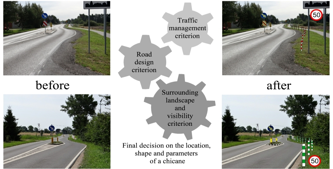
Table 1.
Coefficients of correlation between the vehicle speed after the chicane and reduction in speed ∆v and the amount of the horizontal shift of traffic lane a and the l/2a ratio in relation to the test section data.
Table 1.
Coefficients of correlation between the vehicle speed after the chicane and reduction in speed ∆v and the amount of the horizontal shift of traffic lane a and the l/2a ratio in relation to the test section data.
| Correlation Coefficients in Relation to Conclusions Given in [27] | Correlation Coefficients in Relation to Conclusions Given in [32] | ||||||
|---|---|---|---|---|---|---|---|
| v85 = f (a) | ∆v85 = f (a) | vav = f (a) | ∆vav = f (a) | v85 = f (l/2a) | ∆v85 = f (l/2a) | vav = f (l/2a) | ∆vav = f (l/2a) |
| 0.18 | −0.36 | 0.17 | −0.27 | 0.5 | −0.33 | −0.07 | −0.29 |
Table 2.
Coefficients of correlation R between the quantitative measures and the chosen speed distribution parameters (including the additional sections No. 11 and No. 12).
Table 2.
Coefficients of correlation R between the quantitative measures and the chosen speed distribution parameters (including the additional sections No. 11 and No. 12).
| v85before | vavbefore | vav pp before | v85after | vavafter | vav pp after | ∆v85 | ∆vav | ∆vav pp | w (v85) | w (vav) | |
|---|---|---|---|---|---|---|---|---|---|---|---|
| zzw | −0.35 | −0.27 | −0.33 | −0.78 | −0.78 | −0.80 | 0.81 | 0.92 | 0.89 | 0.84 | 0.92 |
| zd | −0.31 | −0.29 | −0.35 | −0.72 | −0.74 | −0.79 | 0.77 | 0.83 | 0.85 | 0.81 | 0.85 |
| zo | −0.23 | −0.20 | −0.33 | −0.56 | 0.66 | 0.71 | 0.61 | 0.66 | 0.71 | 0.63 | 0.67 |
| z | −0.35 | −0.29 | −0.37 | −0.79 | −0.80 | −0.86 | 0.84 | 0.93 | 0.93 | 0.87 | 0.94 |
Table 3.
Coefficients of correlation R between the quantitative measures and the chosen speed distribution parameters (excluding the additional sections No. 11 and No. 12, which had no chicanes installed).
Table 3.
Coefficients of correlation R between the quantitative measures and the chosen speed distribution parameters (excluding the additional sections No. 11 and No. 12, which had no chicanes installed).
| v85before | vavbefore | vav pp before | v85after | vavafter | vav pp after | ∆v85 | ∆vav | ∆vav pp | w (v85) | w (vav) | |
|---|---|---|---|---|---|---|---|---|---|---|---|
| zzw | −0.10 | −0.12 | −0.10 | −0.67 | −0.67 | −0.67 | 0.86 | 0.89 | 0.83 | 0.88 | 0.89 |
| zd | −0.06 | −0.17 | −0.16 | −0.59 | −0.62 | −0.67 | 0.78 | 0.77 | 0.77 | 0.80 | 0.77 |
| zo | 0.05 | −0.05 | −0.13 | −0.35 | −0.37 | −0.49 | 0.56 | 0.60 | 0.55 | 0.56 | 0.50 |
| z | −0.07 | −0.15 | −0.16 | −0.70 | −0.72 | −0.77 | 0.94 | 0.92 | 0.92 | 0.96 | 0.93 |
Publisher’s Note: MDPI stays neutral with regard to jurisdictional claims in published maps and institutional affiliations. |
© 2021 by the authors. Licensee MDPI, Basel, Switzerland. This article is an open access article distributed under the terms and conditions of the Creative Commons Attribution (CC BY) license (https://creativecommons.org/licenses/by/4.0/).
Share and Cite
MDPI and ACS Style
Sołowczuk, A.B.; Kacprzak, D. Identification of the Determinants of the Effectiveness of On-Road Chicanes in the Village Transition Zones Subject to a 50 km/h Speed Limit. Energies 2021, 14, 4002. https://doi.org/10.3390/en14134002
AMA Style
Sołowczuk AB, Kacprzak D. Identification of the Determinants of the Effectiveness of On-Road Chicanes in the Village Transition Zones Subject to a 50 km/h Speed Limit. Energies. 2021; 14(13):4002. https://doi.org/10.3390/en14134002
Chicago/Turabian StyleSołowczuk, Alicja Barbara, and Dominik Kacprzak. 2021. "Identification of the Determinants of the Effectiveness of On-Road Chicanes in the Village Transition Zones Subject to a 50 km/h Speed Limit" Energies 14, no. 13: 4002. https://doi.org/10.3390/en14134002
Note that from the first issue of 2016, this journal uses article numbers instead of page numbers. See further details here.