
Optimal Air Conditioner Placement Using a Simple Thermal Environment Analysis Method for Continuous Large Spaces with Predominant Advection


1
Kurume Institute of Technology, 2228-66 Kurume City, Kurume 830-0052, Fukuoka, Japan
2
Graduate School of Human-Environment Studies, Kyushu University, 744 Motooka, Nishi-ku 819-0395, Fukuoka, Japan
3
Department of Science and Engineering, Ritsumeikan University, 1-1-1 Noji-higashi, Kusatsu 525-8577, Shiga, Japan
*
Author to whom correspondence should be addressed.
Energies 2021, 14(15), 4663; https://doi.org/10.3390/en14154663
Submission received: 24 June 2021
/
Revised: 22 July 2021
/
Accepted: 28 July 2021
/
Published: 31 July 2021
(This article belongs to the Special Issue Advanced Environmental Controls for High-Performance Buildings and Sustainability)
Abstract
:The number of houses with large, continuous spaces has increased recently. With improvements in insulation performance, it has become possible to efficiently air condition such spaces using a single air conditioner. However, the air conditioning efficiency depends on the placement of the air conditioner. The only way to determine the optimal placement of such air conditioners is to conduct an experiment or use computational fluid dynamic analysis. However, because the analysis is performed over a limited period, it is difficult to consider non-stationarity effects without using an energy simulation. Therefore, in this study, energy simulations and computational fluid dynamics analyses were coupled to develop a thermal environment analysis method that considers non-stationarity effects, and various air conditioner arrangements were investigated to demonstrate the applicability of the proposed method. The accuracy verification results generally followed the experimental results. A case study was conducted using the calculated boundary conditions, and the results showed that the placement of two air conditioners in the target experimental house could provide sufficient air conditioning during both winter and summer. Our results suggest that this method can be used to conduct preliminary studies if the necessary data are available during design or if an experimental house is used.
1. Introduction
In recent years, the number of large, continuous spaces in both homes and offices has increased. For example, in homes, the use of atrium spaces is increasing. Convection air conditioners account for most air conditioners in residential buildings, and their use continues to increase; there are now few dwellings without air conditioning. Energy simulation (ES) and computational fluid dynamics (CFD) are two examples of thermal environment simulations that are used during design. There are many examples of CFD analysis for air conditioners with highly directional advection [1,2]. In ES, calculations can also be performed by setting an air conditioning schedule. However, the general assumption is that there are many individual rooms, rather than a continuous large space.
Large spaces such as atria have also been analyzed, but the analyses are limited to CFD [3,4]. Recent studies have applied CFD, although verification by experiment and analysis has also been conducted [5]. Studies that consider the entire building as a continuous space have also been investigated using CFD [6,7]. Additionally, CFD works well with wind tunnel experiments, and it has been confirmed that the effects of ventilation at openings can be calculated precisely [8].
On the other hand, in ES, there are many cases where building information modeling (BIM) and other methods are used for simulating the energy of an entire building [9,10]. Several studies based on the degree of influence between buildings have also been conducted [11]. These studies focus on buildings and examine the influence of shadows from neighboring buildings. Coupled with equipment such as radiant panels [12], it can be said that ES specializes in energy analysis.
Meanwhile, the meteorological data for 2030 in the near future and 2050 in the medium to long term are also being prepared [13], and the data for the input conditions necessary for both ES and CFD are being developed. In addition, urban TMY (uTMY) data that consider the climate of cities have been created recently, and the calculation results show that the annual energy demand will decrease by 24.1% compared with the conventional TMY [14]. Although the elaborate handling of meteorological data is beyond the scope of this study, it can be considered as an important research background.
Both ES and CFD are currently used for thermal environment analysis in the design field, with CFD being easier to explain to clients. However, ES has the advantage of being able to analyze the thermal environment in a nonstationary manner, and thermal environment analysis methods, such as the heat distribution method [15] and the contribution ratio of indoor climate [16], have been developed. However, these analysis methods are not suitable for practical use because of concerns regarding high analysis loads. In particular, the number of meshes required is so large that it is necessary to prepare a suitable workstation, increasing analysis costs. These thermal environment analysis methods are based on a coupled ES and CFD analysis, which was developed and systematized by Zhai et al. [17,18].
A coupled ES and CFD analysis method for residential buildings, which can track changes over time by dynamic coupling, has been recently proposed [19], and coupled ES and CFD analysis including air conditioning control (PID control) has been conducted in relation to PCM (phase change material). Thus, the range of applications has widened [20]. In addition, some studies have indicated that the microclimate is affected by the height of buildings in urban areas, using coupled ES and CFD, and the knowledge of coupled analysis including urban areas has been accumulated [21]. Such coupled analyses require a huge analytical load, and it is thought that some measures are necessary with the current machine specifications. Recently, knowledge of the prediction accuracy of power consumption by coupling with air conditioning models has been accumulated [22,23]. In particular, coupled analysis has also been conducted for the control of the relative humidity of a space [24], and because CFD analysis is used to reproduce the fine control, it can be said that further development is expected in this field.
General-purpose fluid analysis software such as SCRYU/Tetra [25], which incorporates coupled analysis of human thermal models and CFD, also exists, and the human body effects have been thoroughly evaluated. For thermal comfort, many studies based on CFD coupling with ventilation and daylighting have been conducted [26,27].
It is undeniable that the analysis load will increase if the human body is evaluated. In some cases, it may be possible to present cautious designs if the thermal environment can be understood. However, air conditioners are the main air conditioning equipment used in houses, and heat is transported by directional advection. In buildings with stairwells in particular, the thermal environment depends on the placement of the air conditioner, and, from the perspective of zone division, there is a limit to the precise calculation of heat transport by directional advection using ES. Therefore, separate measures are necessary.
Therefore, in this study, a simple method was developed to reduce the computational load of CFD while tracking actual measured values for use in the design phase. Air conditioner arrangements were then studied, and a case study of the optimal arrangement (in terms of heat and comfort) was conducted. It should be noted that this case study was based on the results of the experiment. The method proposed in this study is a simple analysis method that can be used in architectural design and product development, and it has a wide range of applications.
2. Materials and Methods
2.1. Overview of the Proposed Method
In this study, the thermal environment of residential buildings (THERB) comprising heat, air, and moisture (HAM) [28] was used for ES, and STAR-CCM+ [29] was used for CFD. THERB is a dynamic heat load simulation tool that can perform sophisticated calculations including heat and moisture transfer.
Figure 1 shows the coupled flow. In Step 1, the air conditioning load was calculated by assuming that all zones were isothermally conditioned using THERB. The ratio of the heat load of the entire building to that of each zone is defined as the air conditioning load ratio. In the CFD analysis, the boundary conditions were assumed to be the air conditioning setpoint temperature, and the heat quantity diffusion ratio was calculated considering the effect of advection with the directionality of the air conditioning unit.
It should be noted that the air conditioning load ratio needs to be calculated for each room and from time to time. To calculate the heat volume diffusion ratio, the air conditioning load ratio was multiplied by the heat volume diffusion ratio. The heat load of each zone used in THERB is multiplied by the heat distribution ratio to calculate the room temperature by distributing it to each room (Figure 2).
2.2. Coupled Procedure
As a preparatory step to calculate the heat distribution ratio, the air conditioning load ratio and heat diffusion ratio were calculated. Equation (1) shows the heat balance equation for the entire building load.
The ES introduces heat input to maintain arbitrarily divided zones at a constant temperature. The heat load for the increase in spatial temperature, relative to the reference temperature for the entire space, is expressed in Equation (1). The reference temperature is the isothermal wall temperature, which is a boundary condition for CFD, set as the temperature of the air conditioner. The temperature increase, relative to the reference temperature for each zone, is multiplied by the heat capacity; they are then added together as the heat load, considering their three-dimensionality. Equation (2) shows that the heat load, after correcting for the difference in the spatial average temperature using the temperature ratio, is equal to the heat load of the target zone. This is called the heat distribution ratio.
From Equation (2), the temperature ratio in Equation (3) can be obtained. In other words, it shows the thermal contribution for each zone by CFD.
The load calculated by the ES does not consider the effect of the directional advection of the air conditioner. Therefore, the heat load of each room is calculated precisely by applying a correction using the temperature ratio calculated from the CFD, as expressed in Equation (4).
By rearranging Equation (4), Equation (5) can be obtained. Here, is the air conditioning load ratio (-), which is expressed by dividing the heat load in zone i by the sum of the heat loads in each zone.
If Equation (5) is expressed as the ratio of each zone to the whole, the net heat distribution ratio can be obtained from Equation (5) using Equation (6).
Equation (7) indicates that the heat distribution ratios of each zone add up to one.
Lastly, the heat is distributed to each zone by multiplying the heat distribution ratio according to Equation (8).
The heat input of the air conditioner is the sum of the heat input of each zone.
The heat balance equation for the space is given by Equation (10). In addition to the heat transport of convection from the walls and the introduction of outside air, the heat inputs qi of the air conditioners in each zone are added together.
3. Verification of Accuracy during Winter and Summer
3.1. Experimental Conditions and Building Model
In this study, accuracy verification was performed using actual measurements from a residence with a continuous space constructed in an artificial weather room. As there were many measurement points in the main living room, it was used as the target room of the accuracy verification. The main rooms on the first and second floors were equipped with convection air conditioning. The measurement points are shown in Figure 3, and the wall structures are listed in Table 1.
A stairwell with a staircase was located on the first floor, adjacent to the rooms on the second floor, to simplify the spatial configuration. Each room was equipped with a convection air conditioner and radiant air conditioning panels. In addition, floor heating was installed only in the first-floor rooms, with a floor installation rate of 70%. In this study, the “living room” was the room colored in gray.
At each measurement point, the temperature in the space, surface temperature, air velocity, and the glove temperature were measured at 1 min intervals. The measuring points a1–d4 are the four points of heights FL + 100, +600, +1100, and +1700, and the measuring points LD1 and LD2 are the seven points of heights FL + 0, +100, +600, +1100, +1700, +2300, and +2400. The measurement point LDwh has nine points of heights FL + 0, +100, +600, +1100, +1700, +2800, +3800, +5000, and CL-0. The measurement points f–i are five points of heights +100, +650, +1200, +1750, and CL-100. These are all related to the height direction, and the vertical temperature distribution was measured.
The average thermal transmittance of the exterior skin of the experimental house was U_A = 0.58 W/m2·K. This satisfies the net zero energy house standard [30] of the Japanese energy conservation standards for regions 4–7 (average external thermal transmittance coefficient U_A = 0.6 W/m2·K), and it would be considered a high level of thermal insulation worldwide.
In this study, the volume-weighted average room temperatures from the simulation were compared with the bulk temperatures calculated from the actual measurements from the main rooms. Therefore, a certain degree of error is considered acceptable without preventing accuracy verification.
3.2. Analysis Details and Conditions
The experimental conditions are listed in Table 2. Only the first-floor air conditioner was operational during the winter analysis, whereas only the second-floor air conditioner was operational during the summer analysis. As for the experimental results, only the volume-weighted average temperature at the time of accuracy verification is reported in this study.
The analysis conditions for THERB are listed in Table 3. The meteorological data were analyzed using actual measurements. The air conditioning temperature was set to 20 °C in winter and 26 °C in summer. The preliminary calculations included 7 days, with 11 January as the target date (the date on which the calculations were performed) in winter and 25 August as the target date in summer. As the analysis method is classified as simple, some differences in the results are expected, depending on the temperature settings. This is because the temperature needed to be lowered during the summer months to obtain accurate verification results. However, it is unlikely that a slight difference in the setpoint temperature would result in a large error in the calculation results. Nevertheless, to elaborate the case study, the setpoint temperature was changed to that which better tracked the accuracy verification results. In other words, the accuracy verification was conducted for elaborate case studies.
Therefore, it should be noted that the proposed method cannot be used in a case study without the existence of experimental results. However, the proposed method still has a wide range of applications, and, depending on how it is used, it can lead to huge savings in experimental time and costs. For example, if a simple method such as this is applied using conservative temperature settings, it is assumed that useful data can be obtained for seasonal design. Table 4 lists the conditions of the CFD analysis. For the boundary conditions of the air vents, the experimental results were input. The input air velocity was calculated from the experimental values of the rotational speed of the outdoor unit. The turbulence model used was a low-Reynolds-number k–ε model, but the proposed method is expected to show no differences in analysis accuracy even if a standard k–ε model with wall functions is used. This is because all the boundary conditions were set to the same temperature. A more detailed turbulence model was chosen as a cautionary measure.
3.3. Overview of the Analyzed Model
Figure 4 shows the THERB and CFD analytical models. The first and second floors were modeled. The spatial configuration was modeled as consistent, and the numbering and zones correspond to each other. As this is a simple method, it is not suitable for analyzing temperature distributions because the CFD wall boundary conditions are constant. It should be noted that this is an analysis method based on nonstationary calculations. However, the proposed method can also be used in the basic design phase without any experimental data. Following the analysis of the results, there are several possible applications of the proposed method, which are summarized in the conclusion.
3.4. Analysis Results and Discussion
3.4.1. Calorific Diffusion Coefficient
Figure 5 shows the calculation results for the heat-rate diffusion coefficient. The effect of directional advection, which cannot be fully accounted for in ES, is corrected by the heat distribution ratio according to the CFD analysis. The heat diffusion coefficients are well balanced and varied, but the values for the air conditioning load and heat diffusion ratio in winter are large in Zones 4 and 6 (the main rooms). In summer, the heat diffusion ratios were large in Zones 6 and 9. The heat probably stayed in Zone 9 because the angle was set to 0° from the horizontal plane, causing a downward flow after colliding with the wall.
3.4.2. Accuracy Verification Results for the First and Second Floors
Figure 6 shows the calculation results of Step 2 in Zones 4 (first floor) and 6 (second floor), using the heat distribution ratios obtained in Step 1. These zones both contained many actual measurement points. The variation in the room temperature in winter and summer indicates that the system tracked these changes well. There was a slight deviation from the actual measurements when the outdoor air temperature was high, but this was thought to be caused by the air conditioner controlling the air volume, which fluctuates with load fluctuation. Depending on the precision of the calculations, this method is affected only slightly by the operational control of the air conditioner in response to fluctuations in outdoor air temperatures.
3.4.3. CFD Results for Temperature and Air Velocity Distribution
Figure 7 shows the results of the CFD air velocity and temperature distributions. The temperature distribution was formed under the influence of strongly directional advection. The heat was not effectively transported to the second floor during winter. Similarly, in summer, the temperature on the first floor was high, although there was an influence of downward flow. Because there was no significant difference in temperature between the first and second floors in the volume-weighted average accuracy results (Figure 6), the wind direction was considered an important factor. As our focus was the heat distribution ratio captured by each zone, we did not verify the accuracy of the airflow temperature distribution. Accuracy verification of the measurement points was also not considered meaningful.
4. Case Study: Optimal Placement of Air Conditioners
4.1. Overview of Placement Study
A building with a stairwell had a continuous spatial configuration, and the indoor thermal environment differed greatly depending on the operating status of the air conditioners on the first and second floors. The optimal placement of the air conditioners in the target building was clarified in this study by conducting a case study using the operating position of the air conditioners as a variable. This study has considerable significance as a case study for orientation during the design stage.
4.2. Analysis Details and Conditions
4.2.1. Analysis Conditions
Table 5 shows the calculation conditions for THERB, assuming that the CFD analysis conditions did not differ from those in Table 4. The total heat input of the air conditioner in this case was the total load when the entire building was air-conditioned at the same temperature. The setpoint temperature during accuracy verification was set to 20 °C in winter and 26 °C in summer, and the same values were used in the case study. The number of ventilation events with outside air was set to 0.5 times/h, and internal heat generation was not considered. The CFD was conducted by changing the arrangement of air conditioners in each case to determine the optimal arrangement. For generalization purposes, the air conditioners on the first floor were operated in winter and those on the second floor were operated in summer.
4.2.2. Details of the Case Study
Figure 8 shows the locations of the air conditioners. The height of the air conditioners was 2 m at the bottom. The cases were set up assuming that only the air conditioner on the first floor was operational in winter and only the one on the second floor was operational in summer. Case A had the same arrangement as that of the experimental house. The air conditioner in Case A was installed perpendicular to the atrium. In contrast, Case A′ was designed to operate only in summer.
It was decided that evaluation by the predicted mean vote (PMV) would be the best way to compare cases; PMV comfort evaluations of the main living room were compared. The PMV is a comfort index based on six factors (temperature, humidity, radiation, air velocity, activity, and clothing), and it is used to evaluate the comfort in a moderate temperature thermal environment that is neither hot nor cold. The PMV is specified in ISO 7730 [31]. More studies are considering approaches to air quality, acoustics, and lighting in addition to thermal comfort [32]. However, it is not ideal to use only CFD for nonstationary analysis [33].
The air velocity of the PMV was set as the volume-weighted average temperature of each zone of the CFD. The temperature and air velocity distributions of the CFD were not considered to represent real phenomena because the boundary conditions of the wall surface were isothermal. The purpose of the CFD is to understand the contribution of heat transport for unsteady calculations; thus, it is desirable to evaluate the CFD using the heat content distribution ratio. Therefore, in this section, we used the heat distribution ratio to evaluate the heat that reached each zone.
It is better for relative evaluations to compare cases using the rate of occurrence of PMV periods, rather than showing changes over time; therefore, cases were compared in this study by the rate of occurrence of PMV periods.
4.3. Analysis Results and Discussion
It was assumed that the main rooms are on 1F (Zone 4) and 2F (Zone 6) in all cases.
4.3.1. Inter-Case Comparison of Heat Distribution Ratios in Winter
Figure 9 shows a comparison of the heat distribution ratios in winter. The air conditioning load ratio had a strong impact on the heat distribution ratio throughout the entire system. In Case B, the values of the air conditioning load ratio and the heat volume diffusion ratio were large in Zones 4 and 6, the residential areas on the first floor. In Case C, the heat distribution ratio was large in Zone 7. Except for Case C, the heat distribution ratios of Zones 4 and 6 were large. This may be because the air conditioners in Case C were placed in a more orthogonal direction to the atrium space than those in the other cases.
It should be noted that the room temperature variation was preliminary, and it was not the primary comparative study. Figure 10 shows the room temperature change over time in the living area of the first-floor room and near the floor on the first day of the calculation period for the calculation results of Step 2 for each case. Because cold feet are a problem in winter, we also considered the feet only in winter. The room temperature was the highest in Case B. This is thought to be because the air from the air conditioner was sufficiently diffused on the first floor as the air did not flow into the atrium. In all cases, the temperature near the floor was low. Thus, it can be seen that low-temperature air flowed into the foot area. Figure 11 shows the room temperature changes over time in the first-floor living area and the second room at the same time. In Case B in Figure 11, the room temperature on the first floor was higher than that on the second floor, and the temperature difference was larger. On the other hand, in Case A, the temperature difference between the first and second floors was relatively small. In Case C, the room temperature of the second floor was higher than that of the first floor. It can be said that the second-floor room temperature tended to be higher in Case A and Case C because the air-conditioned air rose through the atrium, similar to the change over time in the first-floor room shown in Figure 10. In winter, the room temperature did not fluctuate significantly with respect to the outdoor air temperature.
4.3.2. Comparison of PMV between Cases under Winter Conditions
Figure 12 shows the PMV rates of the occupied areas during the 24 h calculation period, where the following conditions were used to calculate PMV: (1) the temperature and radiant temperature were calculated by THERB, (2) the relative humidity was 40%, (3) the amount of clothing was 1.1 clo, and (4) the metabolic rate was 1 MET. The air velocity is the volume-weighted average of the temperature 500 mm from the wall and within 1800 mm of the inside, and the height of the wall. The PMV is also a comfort index expressed between −3.0 and 3.0, with 0 as neutral. PPD (predicted percentage of dissatisfied) is a discomfort rate used with PMV.
The results show that Case B was the most neutral for the first floor while Case C showed a large PMV value ratio of −1.0 (-) (21%). In other words, the environment was too cool and cold. However, the PMV appearance ratio on the first floor in Case C was lower than neutral. This is thought to be because the average radiant temperature of the wall was small, as solar radiation was not considered in this study to maintain consistency with the accuracy verification.
The results of the analysis for the second floor show that the PMV values were further from neutral than those for the first floor, and the ratio for the second floor in Case B was −1.0 (-), indicating that the warm air flow did not reach the second floor. This is because the air conditioner vent was installed in the atrium space.
In conclusion, Case A was the most effective arrangement for air conditioning the second floor in a well-balanced manner by operating an air conditioner on the first floor, and Case B was the most effective for air conditioning only the first floor, although, in this case, it was necessary to take some measures on the second floor.
4.3.3. Comparison of Heat Distribution Ratios between the Cases in Summer
Figure 13 shows a comparison of the heat distribution ratios between the cases during summer. In Case B, the heat distribution ratio of Zone 6 was high, and the heat distribution ratio of Zone 9 was approximately 0.15 (-). Those of the other zones were generally approximately 0.1 (-), except for Zone 6. In Case C, the heat distribution ratio showed a large value of approximately 0.2 (-) for the first floor. In Case A′, the heat distribution ratio was approximately 0.1 (-) in all zones, which is attributed to the leveled room temperatures. Case A′ showed ideal values in terms of the heat distribution ratio and was considered to be suitable for air conditioning the entire building.
4.3.4. Comparison between Cases under Summer Conditions
In each case in Step 2, the room temperature changed over time in the living area of the first and second floors on the first day of the calculation section, as shown in Figure 14. In Case A and Case B, there was a large temperature difference between the first and second floors, and the room temperature in the second-floor room decreased further. This was because the air from the air conditioner did not flow into the atrium and was sufficiently diffused on the second floor. In Case B, the cold air diffused around the living room on the second floor. In Case C, where the air conditioner was installed in the first-floor atrium, the room temperature in the living area of the first-floor room was lower than that of the second-floor room because the temperature of the air blowing out of the atrium was lower than that of the first-floor room. Furthermore, in Case A’, where the blown air flowed into the atrium, the room temperatures of the first-floor living area (Zone 4) and the second-floor living area (Zone 6) showed a similar trend, and the temperature difference was smaller.
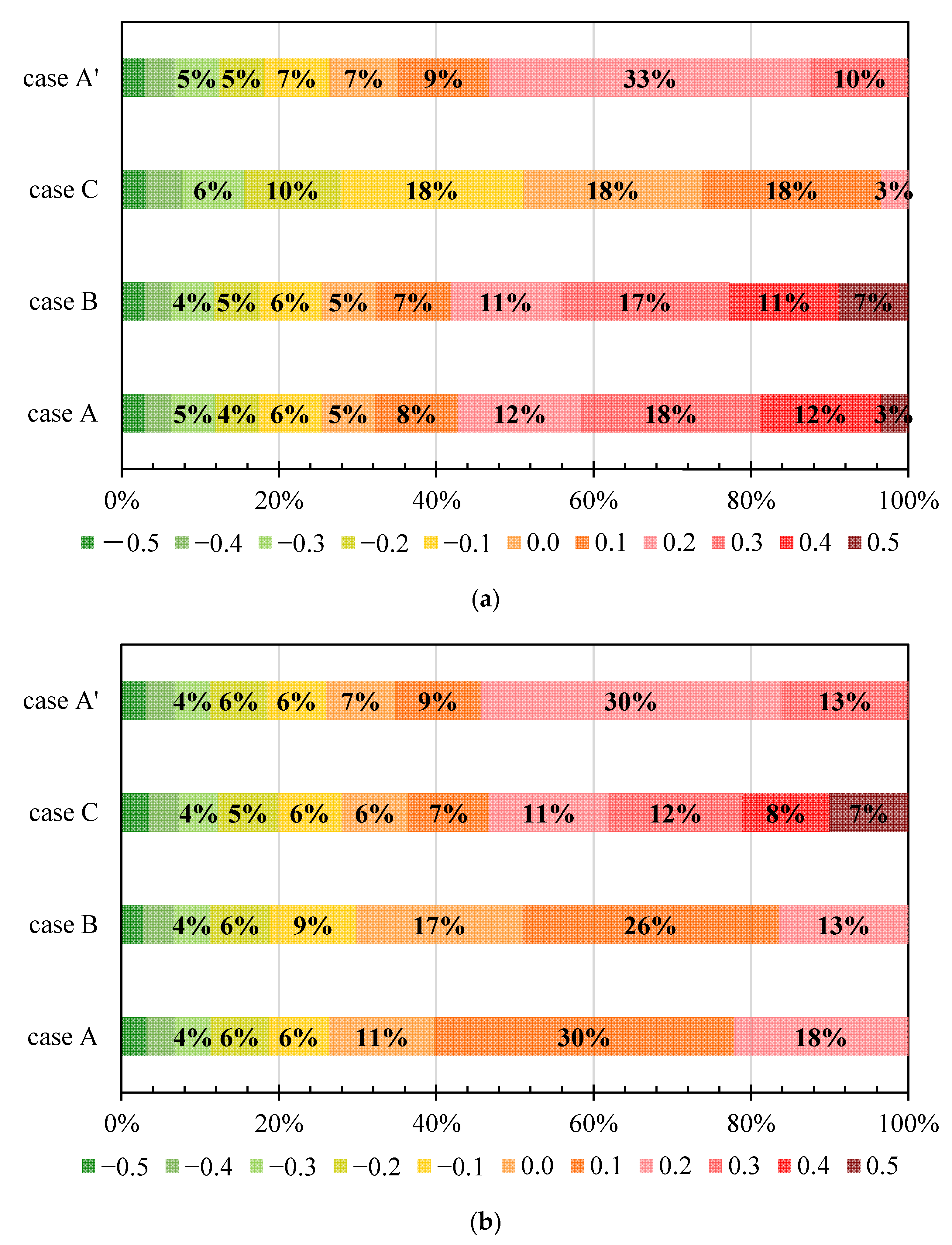
Figure 15 shows the occurrence rate of the PMV on the first and second floors for each case during the calculation period. The calculation conditions for the PMV, temperature, and mean radiant temperature were calculated using THERB. The relative humidity was 60%, the amount of clothing was 0.5 clo, and the metabolic rate was 1 MET from time to time. As in the summer, the air velocity was a volume-weighted average of the air velocity in each zone within 500 mm from the wall and 1800 mm from the inside, and the height of the wall. In Cases A and B, it was inferred that the arrangement on the first floor would not be easily affected by airflow from the air conditioner because the 0.5 (-) appearance ratio was high. In contrast, on the second floor, the values of Cases A and B were close to neutral. Thus, it could be inferred that the second floor was affected by the advection of the air conditioner. Therefore, if one wants to air condition the first and second floors at the same time, Case A′ would be the most effective arrangement. If the second floor did not need to be air-conditioned, the arrangements in Cases A and B would be the most effective because the advection did not affect the atrium space.
5. Discussion
In this study, we developed a simple method to analyze the temperature of each arbitrarily divided zone in a continuous space in an unsteady manner. However, some points to be noted regarding the proposed method are summarized below. It is assumed that the proposed method can be used during the design process, even without experimental data, if conservative settings are established. In addition, the findings of this study can also be applied when accounting for solar radiation. If experimental solar radiation data are available, highly accurate case studies can be conducted. It should be noted that this technology can not only be applied to the building design process, but also to the design of air conditioners.
5.1. Limitations of the Proposed Method
The accuracy of the method was verified during winter and summer. Strictly speaking, it is necessary to add that this is only a simple method, because it was designed for the accuracy verification of a case study. Additionally, a slight deviation from the actual measured values was observed when the outdoor air temperature was high. The air flow rate of the air conditioner was not fully addressed because the control fluctuated according to variations in heat load. However, the calculations at regular time intervals did not deviate significantly from room temperature, meeting the requirements for this study. In this study, no significant error was observed in the calculation of the air flow rate of the air conditioner. Furthermore, there was no significant error; thus, we believe that it is not necessary to perform a coupled calculation at regular time intervals.
Furthermore, the proposed simple method is not capable of reproducing the real phenomenon (temperature distribution) precisely because the boundary conditions of the CFD wall are isothermal. It should be noted that this is a simple method to calculate the contribution of heat to each zone for unsteady calculations. Although this is an ideal method to conduct a case study using settings based on accuracy verification results, it is also possible to conduct a case study alone if the settings are set conservatively. However, the setting conditions must be carefully determined.
Lastly, the results of the case study showed that the wall temperature should be close to the set temperature of the air conditioner. A possible method of setting an appropriate blowing temperature would be to estimate it from the heat load calculated by THERB, using the catalog value of the flow rate. In our case study, this did not cause major problems because relative comparisons were being made.
5.2. Conclusions and Scope for Further Studies
In the case study, the room temperature did not fluctuate significantly in winter. It was possible to evaluate the trends on the first and second floors from a thermal perspective. In the summer season, there were times when the heat input fluctuated rapidly, but it was possible to consider the trend of room temperature fluctuation corresponding to these times. This demonstrates the robustness of the proposed method.
In winter, Case A was effective in efficiently air conditioning the first and second floors, according to the PMV appearance rate. This result can be predicted to some extent by assuming the direction of the advection. However, the proposed method was effective in confirming the subtle sensitivity of areas that were considerably affected by the air conditioner functional power. In summer, it was found that Case A′ had the most balanced air conditioning effect on the first and second floors, in terms of the PMV appearance rate, because of the arrangement of the air conditioners. It is inferred that this resulted from the influence of downdrafts.
Regarding the optimal placement for summer and winter combined, two air conditioners could ideally be installed and used differently depending on the season. Case A would be used for winter and Case A′ for summer. If one wanted to use a single air conditioner to air condition the first and second floors efficiently in both winter and summer, Case A would be preferable. The reason behind this suggestion is that most of the cases were neutral in summer, giving the winter results priority. In this study, the case studies of the winter and summer seasons were conducted by focusing on the PMV. The optimal placement of air conditioners was clearly different between the winter and summer seasons. Thus, it can be inferred that it is ideal to install about two air conditioners for each of the summer and winter seasons. This study showed that it is possible to consider the optimal placement of air conditioners by clarifying the location of the air conditioners at the design stage.
The scope of application of the simple method includes case studies based on experimental data from experimental houses, as well as the use of the analysis results as an indicator of house designs. It is expected that the influence of directional air conditioners and radiant panels can be considered, whereas the possibility of application in large spaces, such as atriums, is fully considered.
In future studies, it is necessary to examine whether this method can be applied to a continuous large space with a standard floor type, such as an office. It is also necessary to confirm how the application of the simple method to a basic design can change the design plan, to demonstrate its applicability. The coupled convective heat transfer coefficient is challenging, and we proposed a simple method; therefore, the boundary conditions of the wall must be reasonable if the method is to be further refined. Because the changes in temperature and humidity control over time are important factors, a more in-depth case study based on the analysis results and consideration of these factors will be conducted in a future work.
Author Contributions
Conceptualization, T.Y. and A.O.; methodology, T.Y.; software, T.Y.; validation, T.Y.; formal analysis, T.Y.; investigation, T.Y.; resources, M.L.; data curation, T.Y.; writing—original draft preparation, T.Y.; writing—review and editing, T.Y. and M.L.; visualization, T.Y.; supervision, A.O.; project administration, M.L.; funding acquisition, A.O. and M.L. All authors read and agreed to the published version of the manuscript.
Funding
This research received no external funding.
Acknowledgments
Technical support for this work was provided by Masahiro Kawabata (former undergraduate student at Kyushu University). We express our gratitude to him.
Conflicts of Interest
The authors declare no conflict of interest.
Nomenclature
| Specific heat of air (J/kg·K) | |
| Specific gravity (kg/m3) | |
| Average space temperature (K) | |
| V | Total area (m3) |
| Zone i volume (m3) | |
| Standard temperature (K) | |
| Spatial average temperature (K) | |
| Ti | Temperature in each zone (K) |
| Ti′ | Temperature in each zone (CFD) (K) |
| Heat dispersion ratio of each chamber (-) | |
| Heat load ratio of each chamber (-) | |
| Thermal diffusivity of each room (-) | |
| Calorimetric diffusion coefficient (-) | |
| qi′ | Air conditioning load of each room (W) |
| qi | Distribution of heat in each room (W) |
| q | Air conditioner input heat (W) |
| Ti,j | Room i, temperature of target element j (K) |
| Apparent volumetric specific heat of rooms containing furniture (J/m3·K) | |
| Si,j | Area of room i, target element j (m2) |
| hi,j | Convective heat transfer coefficient of room i, target element j (W/m2·K) |
| Vo | Ventilation rate with outside air (m3/s) |
References
- Yamamoto, T.; Ozaki, A.; Lee, M. Development of a thermal environment analysis method for a dwelling containing a colonnade space through coupled energy simulation and computational fluid dynamics. Energies 2019, 12, 2560. [Google Scholar] [CrossRef] [Green Version]
- Zhang, W.; Hiyama, K.; Kato, S.; Ishida, Y. Building energy simulation considering spatial temperature distribution for nonuniform indoor environment. Build. Environ. 2013, 63, 89–96. [Google Scholar] [CrossRef]
- Aryal, P.; Leephakpreeda, T. CFD analysis on thermal comfort and energy consumption effected by partitions in air-conditioned building. Energy Procedia 2015, 79, 183–188. [Google Scholar] [CrossRef] [Green Version]
- Li, Q.; Yoshino, H.; Mochida, A.; Lei, B.; Meng, Q.; Zhao, L.; Lun, Y. CFD study of the thermal environment in an air-conditioned train station building. Build. Environ. 2009, 44, 1452–1465. [Google Scholar] [CrossRef] [Green Version]
- Gan, G.; Riffat, S.B. CFD modeling of air flow and thermal performance of an atrium integrated with photovoltaics. Build. Environ. 2004, 39, 735–748. [Google Scholar] [CrossRef]
- Ji, Y.; Cook, M.J.; Hanby, V. CFD modeling of natural displacement ventilation in an enclosure connected to an atrium. Build. Environ. 2007, 42, 1158–1172. [Google Scholar] [CrossRef]
- Ray, S.D.; Gong, N.W.; Glicksman, L.R.; Paradiso, J.A. Experimental characterization of full-scale naturally ventilation of CFD simulations. Energ. Build. 2014, 69, 285–291. [Google Scholar] [CrossRef]
- Fini, A.S.; Moosavi, A. Effects of “wall angularity of atrium” on “buildings natural ventilation and thermal performance” and CFD model. Energ. Build. 2016, 121, 265–283. [Google Scholar] [CrossRef]
- Al-Waked, R.; Nasif, M.; Groenhout, N.; Partridge, L. Natural ventilation of residential building Atrium under fire scenario. Case Stud. Therm. Eng. 2021, 26, 101041. [Google Scholar] [CrossRef]
- Lo, L.J.; Banks, D.; Novoselac, A. Combined wind tunnel and CFD analysis for indoor airflow prediction of wind-driven cross ventilation. Build Environ. 2013, 60, 12–23. [Google Scholar]
- Tushar, Q.; Bhuiyan, M.A.; Zhang, G.; Maqsood, T. An integrated approach of BIM-enabled LCA and energy simulation: The optimized solution towards sustainable development. J. Clean. Prod. 2021, 289, 125622. [Google Scholar] [CrossRef]
- Andriamamonjy, A.; Saelens, D.; Klein, R.A. A combined scientometric and conventional literature review to grasp the entire BIM knowledge and its integration with energy simulation. J. Build. Eng. 2019, 22, 513–527. [Google Scholar] [CrossRef]
- Ascione, F.; Bianco, N.; Iovane, T.; Mastellone, M.; Mauro, G.M. Is it fundamental to model the inter-building effect for reliable building energy simulations? Interaction with shading systems. Build. Environ. 2020, 183, 107161. [Google Scholar] [CrossRef]
- Yu, X.; Chen, C. Coupling spectral-dependent radiative cooling with building energy simulation. Build. Environ. 2021, 197, 107841. [Google Scholar] [CrossRef]
- Pulkkinen, J.; Louis, J.N. Near-and medium-term hourly morphed mean and extreme future temperature datasets for Jyväskylä, Finland, for building thermal energy demand simulations. Data Brief 2021, 37, 107209. [Google Scholar] [CrossRef]
- Tang, Y.; Sun, T.; Luo, Z.; Omidvar, H.; Theeuwes, N.; Xie, X.; Xiong, J.; Yao, R.; Grimmond, S. Urban meteorological forcing data for building energy simulation. Build. Environ. 2021, 204, 108088. [Google Scholar] [CrossRef]
- Zhai, Z.; Chen, Q.; Haves, P.; Klems, J.H. On approaches to couple energy simulation and computational fluid dynamics programs. Build. Environ. 2002, 37, 857–864. [Google Scholar] [CrossRef]
- Zhai, Z.; Chen, Q. Solution characters of coupling between energy simulation and CFD programs. Energy Build. 2003, 35, 493–505. [Google Scholar] [CrossRef]
- Barbason, M.; Reiter, S. Coupling building energy simulation and computational fluid dynamics: Application to a two-storey house in a temperate climate. Build. Environ. 2014, 75, 30–39. [Google Scholar] [CrossRef]
- Gowreesunker, B.L.; Tassou, S.A.; Kolokotroni, M. Coupled TRNSYS-CFD simulations evaluating the performance of PCM plate heat exchangers in an airport terminal building displacement conditioning system. Build. Environ. 2013, 65, 132–145. [Google Scholar] [CrossRef] [Green Version]
- Allegrini, J.; Carmeliet, J. Coupled CFD and building energy simulations for studying the impacts of building height topology and buoyancy on local urban microclimates. Urban. Clim. 2017, 21, 278–305. [Google Scholar] [CrossRef]
- Fan, Y.; Ito, K. Energy consumption analysis intended for real office space with energy recovery ventilator by integrating BES and CFD approaches. Build. Environ. 2012, 52, 57–67. [Google Scholar] [CrossRef]
- Fan, Y.; Ito, K. Integrated building energy computational fluid dynamics simulation for estimating the energy-saving effect of energy recovery ventilator with CO2 demand-controlled ventilation system in office space. Indoor Built Environ. 2014, 23, 785–803. [Google Scholar] [CrossRef]
- Ascione, F.; Bellia, L.; Capozzoli, A. A coupled numerical approach on museum air conditioning: Energy and fluid-dynamic analysis. Appl. Energ. 2013, 103, 416–427. [Google Scholar] [CrossRef]
- SCRY/Tetra. Available online: https://www.cradle.co.jp/product/scryutetra.html (accessed on 4 June 2021).
- Rabani, M.; Madessaa, H.B.; Nord, N.; Schild, P.; Mysen, M. Performance assessment of all-air heating in an office cubicle equipped with an active supply diffuser in a cold climate. Build. Environ. 2019, 156, 123–136. [Google Scholar] [CrossRef]
- Rabani, M.; Madessa, H.B.; Nord, N. Building retrofitting through coupling of building energy simulation-optimization tool with CFD and daylight programs. Energies 2021, 14, 2180. [Google Scholar] [CrossRef]
- Ozaki, A.; Watanabe, T.; Hayashi, T.; Ryu, Y. Systematic analysis on combined heat and water transfer through porous materials based on thermodynamic energy. Energy Build. 2001, 33, 341–350. [Google Scholar] [CrossRef]
- STAR-CCM+. Available online: https://www.plm.automation.siemens.com/global/ja/products/simcenter/STAR-CCM.html (accessed on 4 June 2021).
- Agency for Natural Resources and Energy. Available online: https://www.enecho.meti.go.jp/category/saving_and_new/saving/assets/pdf/general/housing/zeh_definition_kodate.pdf (accessed on 4 June 2021).
- ISO7730. Available online: https://www.iso.org/standard/39155.html (accessed on 4 June 2021).
- Fantozzi, F.; Rocca, M. An extensive collection of evaluation indicators to assess occupants’ health and comfort in indoor environment. Atmosphere 2020, 11, 90. [Google Scholar] [CrossRef] [Green Version]
- Morón, C.; Saiz, P.; Ferrández, D.; Felices, R. Comparative analysis of infrared thermography and CFD modelling for assessing the thermal performance of buildings. Energies 2018, 11, 638. [Google Scholar] [CrossRef] [Green Version]
Figure 1.
Coupled flow of the proposed method. ES, energy simulation; CFD, computational fluid dynamics.
Figure 1.
Coupled flow of the proposed method. ES, energy simulation; CFD, computational fluid dynamics.

Figure 2.
Conceptual diagram of coupled analysis with calorimetric correction: (a) air conditioning load of each room; (b) temperature distribution (computational fluid dynamics); (c) heat input to each room.
Figure 2.
Conceptual diagram of coupled analysis with calorimetric correction: (a) air conditioning load of each room; (b) temperature distribution (computational fluid dynamics); (c) heat input to each room.

Figure 3.
Floor plans and experimental measurement points for the first and second floors: (a) first-floor plan and measurement points; (b) second-floor plan and measurement points. FL, floor; CL, ceiling [3].
Figure 3.
Floor plans and experimental measurement points for the first and second floors: (a) first-floor plan and measurement points; (b) second-floor plan and measurement points. FL, floor; CL, ceiling [3].
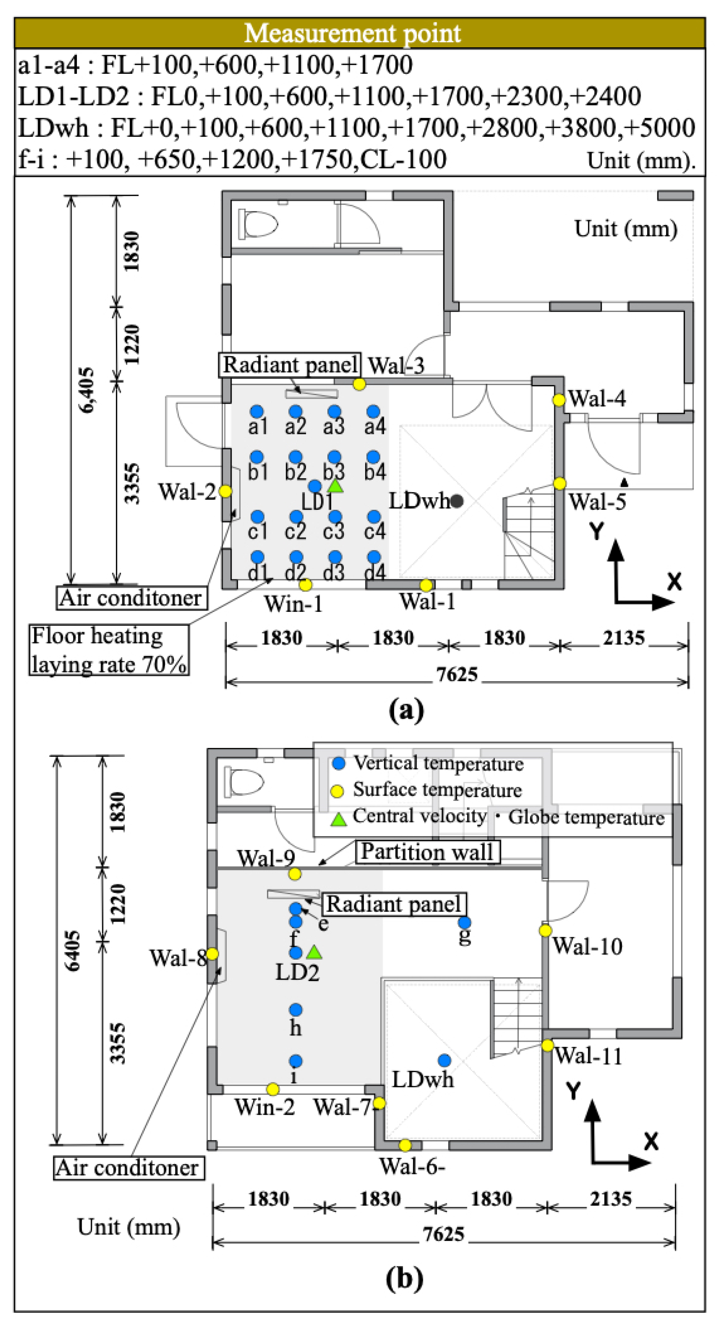
Figure 4.
ES and CFD analysis models: (a) zoning of the ES; (b) CFD analysis model [3].
Figure 4.
ES and CFD analysis models: (a) zoning of the ES; (b) CFD analysis model [3].
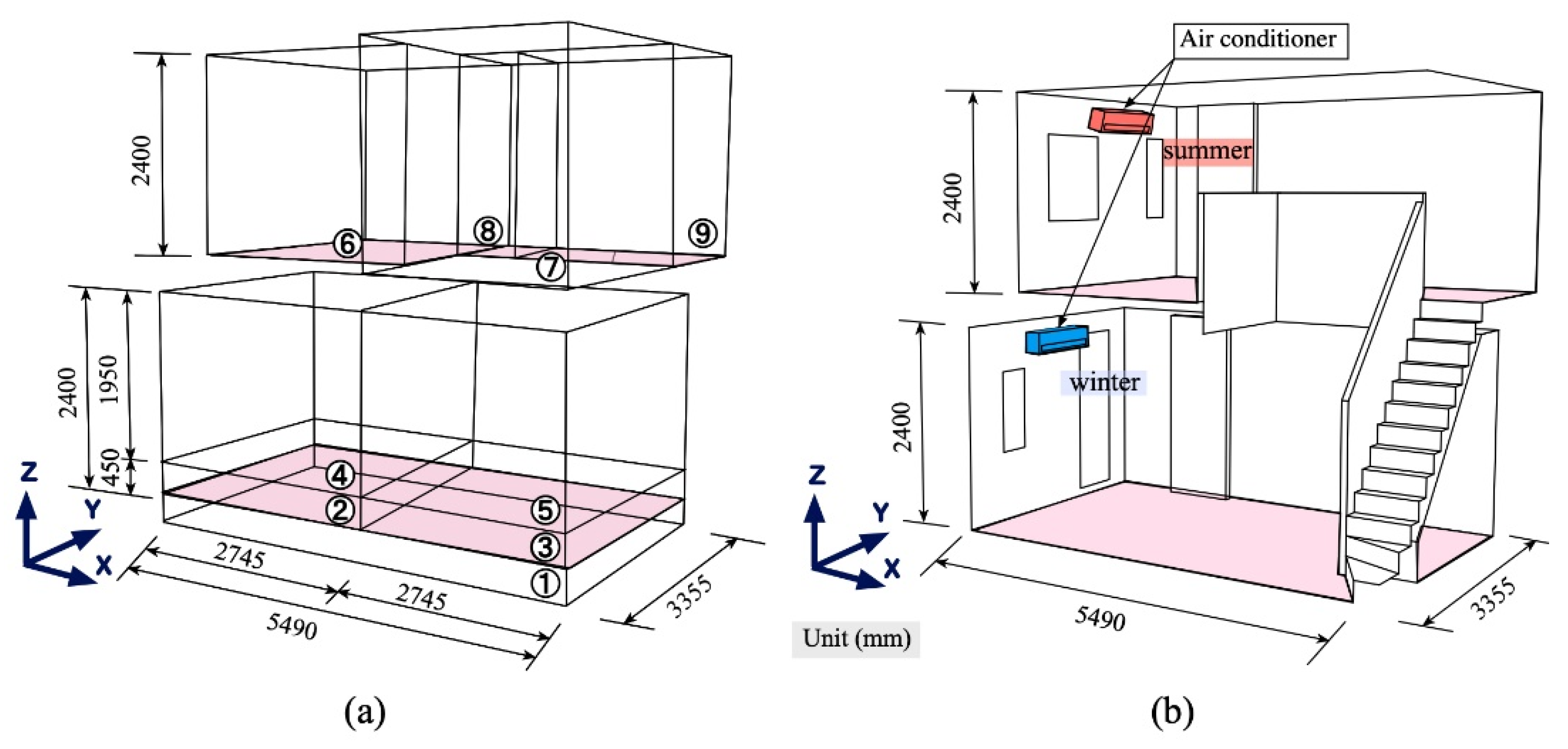
Figure 5.
Calorimetric diffusivity and ratios used in calculations. 1F, first floor; 2F, second floor.
Figure 5.
Calorimetric diffusivity and ratios used in calculations. 1F, first floor; 2F, second floor.

Figure 6.
Results of Step 2 accuracy verification (a) in winter and (b) in summer. 1F, first floor; 2F, second floor.
Figure 6.
Results of Step 2 accuracy verification (a) in winter and (b) in summer. 1F, first floor; 2F, second floor.
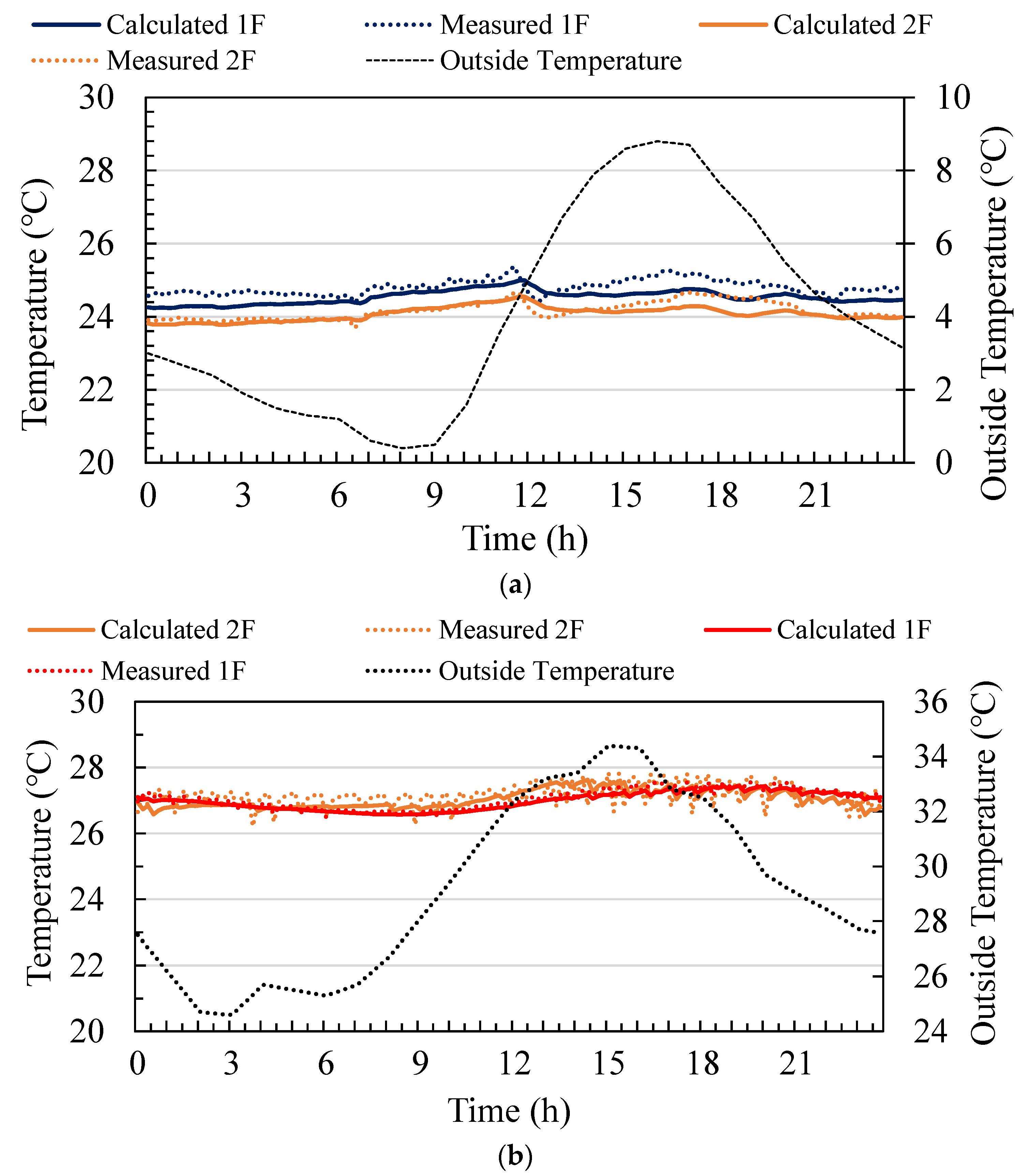
Figure 7.
CFD analysis results: (a) Y-axis 1.5 m, temperature distribution; (b) Y-axis 1.5 m, air velocity distribution; (c) Y-axis 3.27 m, temperature distribution; (d) Y-axis 3.27 m, air velocity distribution.
Figure 7.
CFD analysis results: (a) Y-axis 1.5 m, temperature distribution; (b) Y-axis 1.5 m, air velocity distribution; (c) Y-axis 3.27 m, temperature distribution; (d) Y-axis 3.27 m, air velocity distribution.
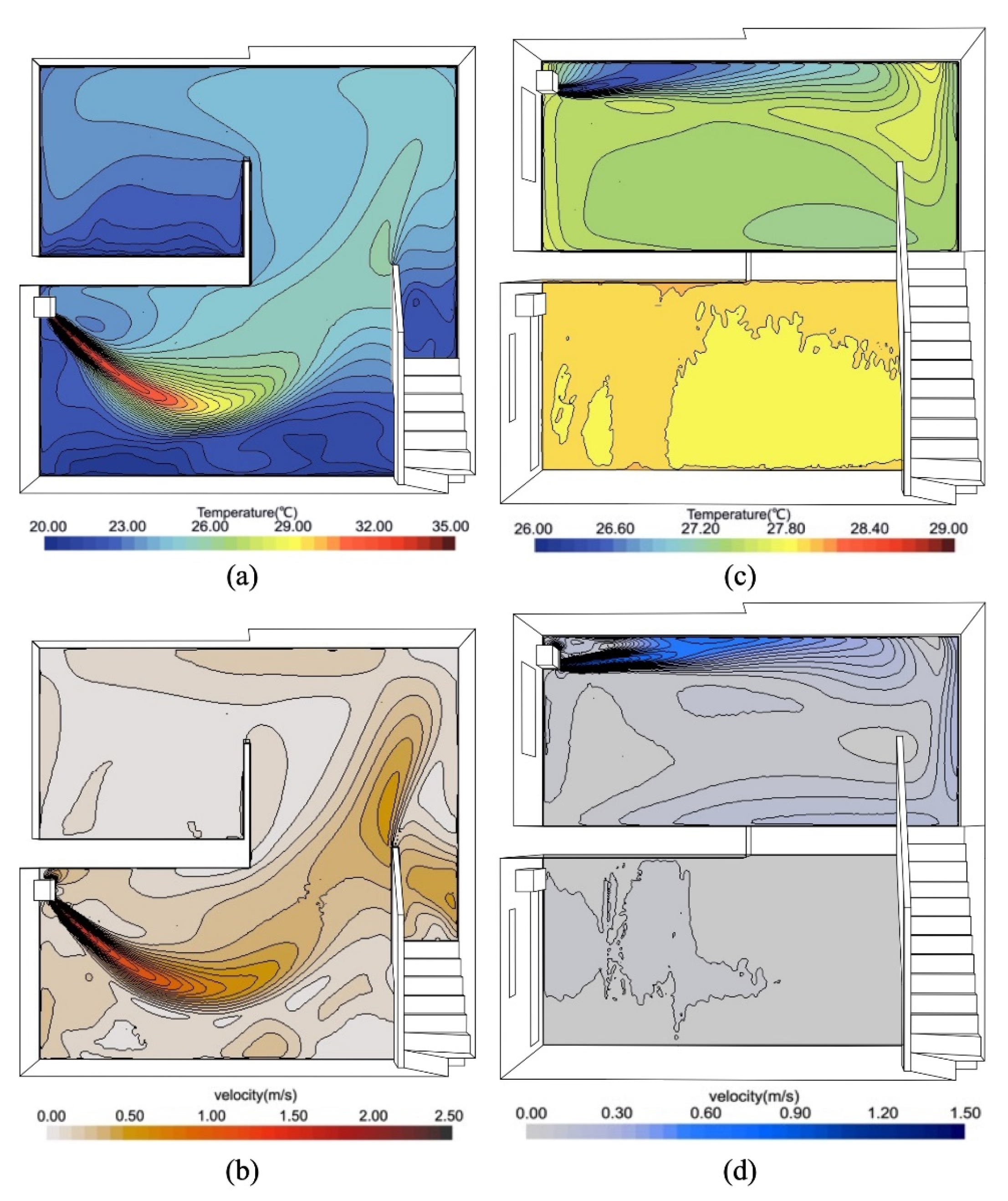
Figure 8.
Air conditioner placement in Cases A, B, C, and A′ (a,b). Shading indicates the air conditioner used in each case.
Figure 8.
Air conditioner placement in Cases A, B, C, and A′ (a,b). Shading indicates the air conditioner used in each case.
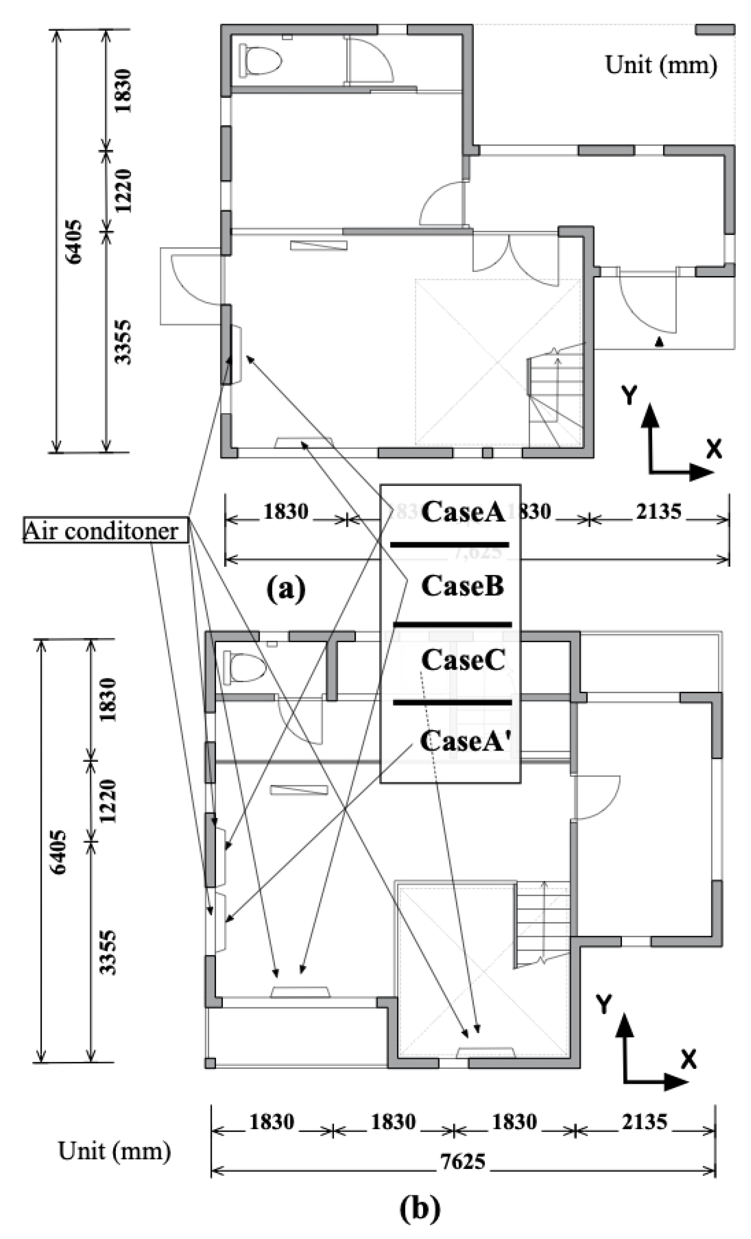
Figure 9.
Inter-case comparison of heat distribution ratios in winter.

Figure 10.
Room temperature change over time in the first-floor living area (Zone 4) and near the floor (Zone 2).
Figure 10.
Room temperature change over time in the first-floor living area (Zone 4) and near the floor (Zone 2).

Figure 11.
Change over time in first-floor living area (Zone 4) and second-floor room (Zone 6) temperature.
Figure 11.
Change over time in first-floor living area (Zone 4) and second-floor room (Zone 6) temperature.

Figure 12.
Inter-case comparison of heat distribution ratios in winter: (a) first-floor residential domain PMV presence ratio; (b) PMV occurrence rate on the second floor.
Figure 12.
Inter-case comparison of heat distribution ratios in winter: (a) first-floor residential domain PMV presence ratio; (b) PMV occurrence rate on the second floor.

Figure 13.
Comparison of heat distribution ratios between cases in summer.

Figure 14.
Room temperature change over time in the This is what happens when you set it to minus (-) in Excel. It is impossible to fix.first-floor living area (Zone 4) and second-floor room (Zone 6).
Figure 14.
Room temperature change over time in the This is what happens when you set it to minus (-) in Excel. It is impossible to fix.first-floor living area (Zone 4) and second-floor room (Zone 6).
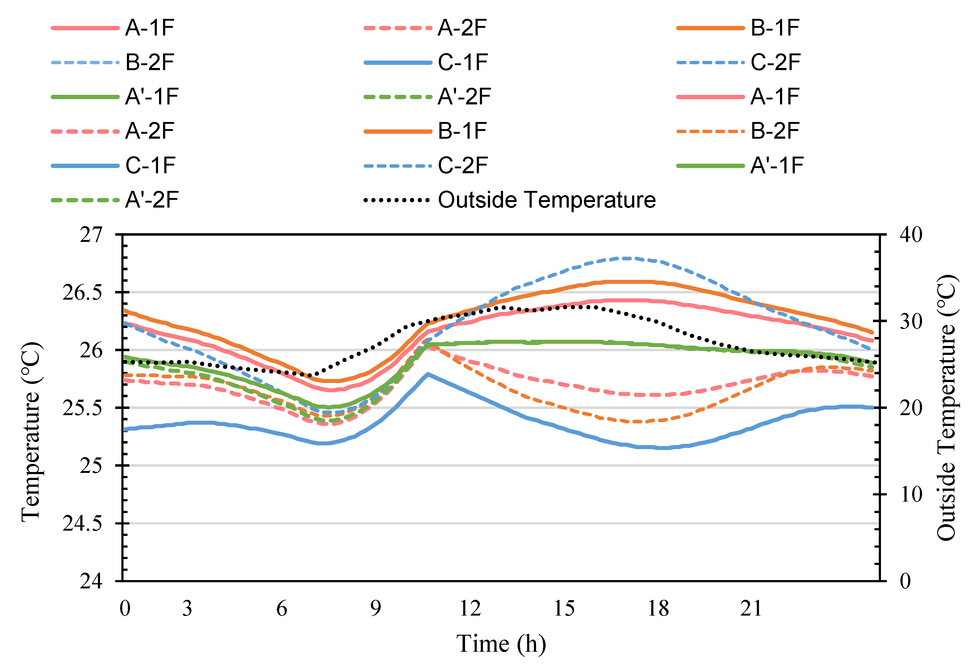
Figure 15.
PMV occurrence rate in residential areas during summer: (a) first-floor residential domain PMV presence ratio; (b) PMV occurrence rate in second-floor s living rooms.
Figure 15.
PMV occurrence rate in residential areas during summer: (a) first-floor residential domain PMV presence ratio; (b) PMV occurrence rate in second-floor s living rooms.

Table 1.
Wall structure.
| Element | Materials | Thickness (mm) | Conductivity (W/m·K) |
|---|---|---|---|
| Foundation wall | RC | 160 | 1.619 |
| Outer wall | plasterboard | 125 | 0.202 |
| phenol foam | 175 | 0.018 | |
| RC | 75 | 1.619 | |
| Inner wall | plasterboard | 12 | 0.202 |
| air layer | 100 | 0.024 | |
| plasterboard | 12 | 0.202 | |
| Window 1 | glass | 3 | 0.780 |
| low-e insulation | - | - | |
| argon gas layer | 16 | 0.0163 | |
| glass | 3 | 0.780 | |
| Window 2 | glass | 3 | 0.780 |
| low-e insulation | - | - | |
| air layer | 16 | 0.024 | |
| glass | 3 | 0.780 | |
| First floor | floor finish | 13 | 0.103 |
| plywood | 12 | 0.103 | |
| extruded polystyrene | 20 | 0.028 | |
| ALC plate | 100 | 0.444 | |
| phenol foam | 100 | 0.018 | |
| Second floor | floor finish | 13 | 0.103 |
| rigid foam | 20 | 0.023 | |
| mortar | 12 | 1.91 | |
| board | 100 | 0.150 | |
| air layer | 340 | 0.024 | |
| plasterboard | 9 | 0.202 | |
| Roof | insulation board | 12 | 0.039 |
| extruded polystyrene foam | 50 | 0.028 | |
| phenol foam | 90 | 0.018 | |
| ALC plate | 75 | 0.444 |
Table 2.
Experimental conditions.
| Item | Conditions | ||
|---|---|---|---|
| Artificial weather chamber setting | Fuchu City, Tokyo | ||
| Ventilation frequency | 0 times | ||
| Air conditioning equipment settings (first and second floors) | Winter | Temperature | 20 °C |
| Summer | 28 °C | ||
| Winter | Wind direction | 45° downward from horizontal plane | |
| Summer | Horizontal direction 0° | ||
| Winter | Air velocity | Strong | |
| Summer | |||
Table 3.
THERB analysis conditions.
| Item | Conditions |
|---|---|
| Calculation time | 10 min |
| Weather data | Measured values |
| Ventilation, number of times | 0 (there was no fresh air inflow) |
| Air conditioning temperature (Step 1) | Winter: 20 °C |
| Summer: 26 °C | |
| Air conditioner injection heat capacity (Step 1) | Calculated from measured values |
Table 4.
CFD analysis conditions.
| Item | Conditions |
|---|---|
| Turbulence model | Low-Reynolds-number k–ε model |
| Mesh | Approximately 3,200,000 |
| Wall boundary | Air conditioner setting temperature |
| Inflow/outflow border | Supply opening (Winter: only first-floor air conditioner operational) Velocity: 2.52 m/s Angle: horizontal direction 45° Ventilation temperature: 40 °C (Summer: only second-floor an air conditioner operational) Velocity: 1.42 m/s Angle: horizontal direction 0° Ventilation temperature: 25.9 °C I = 0.01 v: air velocity (m/s); : model coefficient (-); k: kinetic energy (m2/s2); I: turbulence intensity (-); : Turbulence dispersion rate (m2/s3); : vortex viscosity ratio (-) Return intake/exit flow quantity distribution Distribution ratio: 1.0 |
| CFD code | STAR-CCM+ 11.02.010 |
Table 5.
THERB calculation conditions.
| Item | Condition |
|---|---|
| Calculation time | 10 min |
| Weather data | Winter: 1 January to 31 January |
| Summer: 1 August to 31 August | |
| Ventilation number of times | 0.5 times |
| Air conditioning temperature (Step 1) | Winter: 20 °C |
| Summer: 26 °C | |
| Air conditioner input heat (Step 1) | Winter: 20 °C air conditioning load of the whole building |
| Summer: 26 °C air conditioning load of the whole building |
Publisher’s Note: MDPI stays neutral with regard to jurisdictional claims in published maps and institutional affiliations. |
© 2021 by the authors. Licensee MDPI, Basel, Switzerland. This article is an open access article distributed under the terms and conditions of the Creative Commons Attribution (CC BY) license (https://creativecommons.org/licenses/by/4.0/).
Share and Cite
MDPI and ACS Style
Yamamoto, T.; Ozaki, A.; Lee, M. Optimal Air Conditioner Placement Using a Simple Thermal Environment Analysis Method for Continuous Large Spaces with Predominant Advection. Energies 2021, 14, 4663. https://doi.org/10.3390/en14154663
AMA Style
Yamamoto T, Ozaki A, Lee M. Optimal Air Conditioner Placement Using a Simple Thermal Environment Analysis Method for Continuous Large Spaces with Predominant Advection. Energies. 2021; 14(15):4663. https://doi.org/10.3390/en14154663
Chicago/Turabian StyleYamamoto, Tatsuhiro, Akihito Ozaki, and Myonghyang Lee. 2021. "Optimal Air Conditioner Placement Using a Simple Thermal Environment Analysis Method for Continuous Large Spaces with Predominant Advection" Energies 14, no. 15: 4663. https://doi.org/10.3390/en14154663
Note that from the first issue of 2016, this journal uses article numbers instead of page numbers. See further details here.