Nonlinear Controller for the Set-Point Regulation of a Buck Converter System

Abstract

In this paper, we present a nonlinear PID controller based on saturation functions with variable parameters in order to regulate the output voltage of a buck converter in the presence of changes in the input voltage. The main feature of the proposed controller is to bound the control input with a variable parameter to avoid the windup effect generated by the combination of the integral control action and some operation conditions. The main advantages of the proposed nonlinear PID controller are its low computing cost and the simple tuning task to implement the control strategy in an embedded system. The acceptable behavior of the closed-loop system is presented through the simulation and experimental results.

1. Introduction

The control algorithms implemented in power electronic buck converters have improved the performance of this kind of system under nominal operation conditions, as explained in [1]. One of these nominal conditions is considered in the design process, namely that the input voltage remains constant during the entire operation. However, there are some systems, such as photovoltaics and wind turbines, where it is necessary to use the power electronic buck converter, but the main problem is the variable voltage produced by the temporal obstructions of the sun and wind speed variation, respectively. In some cases, the maximum power point tracking (MPPT) method has been applied to mitigate the above effect, however, this method is focused on maximizing the power output to various systems under different conditions, as described in [2].

In the literature, there are different control strategies to improve the behavior of power converters. For example, a robust optimal power management system for a micro-grid was explained in [3]. In [4], the authors described in detail how sliding mode controllers can be practically engineered to optimize the control of power converters. In [5], the fractional-order terminal sliding-mode control, which has a new fractional-order sliding surface and assures the finite time convergence of the output voltage error to the equilibrium point during the load changes, is presented. Other interesting approaches of the sliding mode control technique for the power electronic converter were explained in [6,7,8,9,10]. In [11], the stability properties and results were given for the steady-state control error offset induced by stationary high-frequency measurement disturbances while operating the control loop close to saturation. In [12], the authors presented diverse alternative methods for the control of power electronic converters applying fractional order control. The controller was carried out by the design of a linear controller for the buck converter and the fractional calculus was proposed to determine the switching surface applying a fractional sliding mode control scheme to the control of such devices. In [13], a comparison between different techniques for the design and implementation of closed-loop control systems for buck converters was carried out. Controllers used for this comparison were integral, proportional plus integral controllers and artificial intelligence was represented in the fuzzy logic controller. Optimal switching between different topologies in step-down direct current–direct current (DC-DC) voltage converters, with non-ideal inductors and capacitors is presented in [14]. A backpropagation neural network to fit the input–output relationship of the offline control laws under different operating points was proposed in [15]. In [16], a mixed-logic dynamic model and control method based on mode selection were proposed for the buck converter. A novel fast model predictive control methodology based on linear parameter varying systems was explained in [17]. In [18], the authors presented a fuzzy logic controller that performs the output voltage regulation of a DC/DC buck power converter. Other interesting approaches of the fuzzy logic control technique for power electronic converters were explained in [19,20,21].

In general, most control strategies do not take into account changes in input voltage, which in combination with a control strategy with integral action, could produce the undesired windup effect in a buck converter. In other words, the windup effect refers to the situation in a PID controller where a large change between the set-point and the output system occurs for a relatively long time; consequently, the integral term accumulates a significant value and the specific problem is the excess overshooting. In [22], the main causes of this effect are described in the control context: the author explains that if the control contains integral action, input saturation can give rise to large and poorly decaying overshoots in the transients, which must be avoided. In the literature, there are control algorithms proposed to prevent the windup effect; for example, in [23], the authors focused on the anti-windup control problem for plants with input saturation, and a delayed decoupling structure was first proposed; then, appropriate linear matrix inequalities were developed to determine a plant-order anti-windup compensator. In [24], a unified framework was presented for the study of linear time-invariant systems subject to control input nonlinearities. The framework was based on the following design paradigm: designing the linear controller ignoring control input nonlinearities, and then adding anti-windup bumpless transfer compensation to minimize the adverse effects of any control input nonlinearities on closed-loop performance. In [25], a design method of robust disturbance feedback control was proposed by a linear matrix inequality, with industrial refrigeration system applications. The important aspects of anti-windup designs, namely the parametrization of linear anti-windup compensators, and the role of artificial nonlinearity in the design of anti-windup compensators for multivariable systems, were in presented [26].

The above control strategies improved the behavior of the buck converter; however, the simplicity to implement these controllers is an important topic for industrial applications. In this context, the proportional–integral–derivative controllers were the most adopted in industrial settings because of the advantageous cost–benefit ratio they are able to provide, as explained in [27]. Furthermore, in the literature, there are different variations of the proportional–integral–derivative controllers to improve the performance of the buck converter system. For example, in [28], the nonlinearity of a saturation was taken into account in a model of DC-DC buck power converters, for which a Lyapunov function-based class of proportional–integral with anti-windup algorithms was given. In [29], an internal model control-based anti-windup compensator was designed for nonlinear systems subjected to time-varying delay and input saturation. A robust nonlinear dynamic anti-windup compensator design for nonlinear systems with parametric uncertainties and one-sided Lipschitz nonlinearities under actuator saturation was presented in [30]. In [31], we proposed a proportional–derivative controller with a saturation function where the parameters are variable, in order to improve the closed-loop system when there are time-variant disturbances; considering the previous work, we proposed a nonlinear PID controller to avoid the windup effect, which appears when the input voltage of the buck converter is time-variant. In summary, the contribution of this work focuses on:

• A novel nonlinear PID controller to avoid the windup effect;
• Simulation and experimental results to show the main advantage of the proposed controller;
• Comparative results between the behavior produced by classical PID and nonlinear PID controllers.

The paper is organized as follows. In Section 2, we describe the buck converter system and the design method to obtain its parameters. Section 3 presents the proposed nonlinear PID controller. The simulation results are given in Section 4. Finally, the conclusions and recommendations for future work are summarized in Section 5.

2. System Description

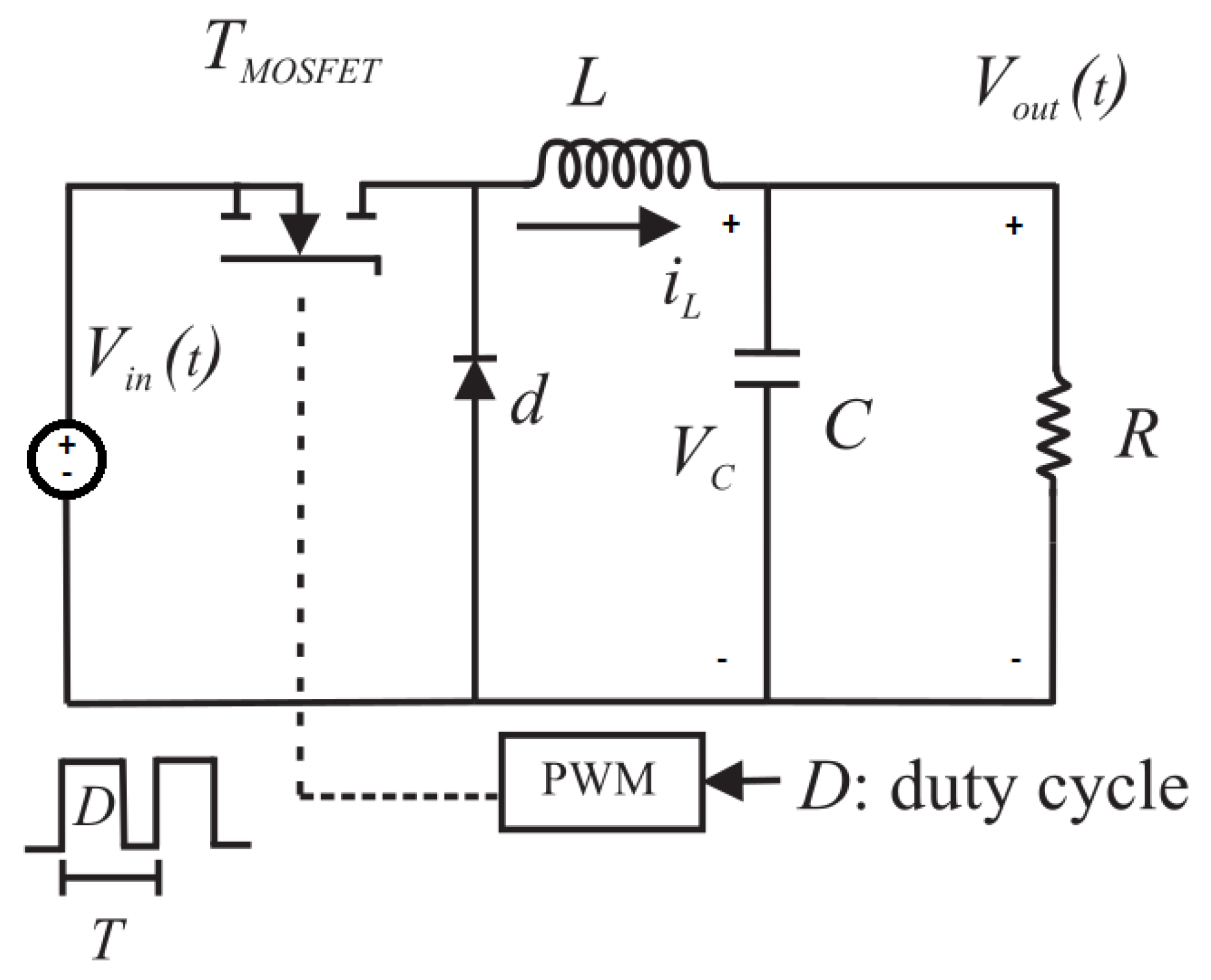
The buck converter system is a very simple type of DC-DC converter that produces an output voltage ($V_{out}\left(t\right)$) that is less than its input voltage ($V_{in}\left(t\right)$). In this section, we describe the general form of that the design process takes to obtain the parameter of the power electronic DC-DC converter and its behavior in the presence of changes in the input voltage. Figure 1 shows the topology of a buck converter, where it notices that this DC-DC converter is composed by a switch power $\left(T_{MOSFET}\right)$, an inductance $\left(L\right)$, a diode $\left(d\right)$, a capacitor $\left(C\right)$ and a load—in this case a resistance $\left(R\right)$. The main goal of the buck converter is to regulate the capacitor voltage $\left(V_c\right)$, where the load is connected, as for this the switch the power is manipulated by a pulse width modulation (PWM) signal with a constant period (T), as explained in [1].

Then, taking into account the general equations for the process design of a buck converter system, as explained in [1], we obtained the parameters that are shown in

Table 1. Buck converter parameters.

$V_{in}\left(t\right)$	=	12 V	$P_{load}$	=	$0.81$ W	$C=$	$3.6\times {10}^{-5}$ F
$V_{out}\left(t\right)$	=	9 V	D	=	$0.75$	$L=$	$3.1\times {10}^{-3}$ H
$\Delta V_{out}\left(t\right)$	=	0.1 V	f	=	5 KHz	$R=$	100 $\Omega$

, assumed that the system is operating under nominal conditions.

Now, in order to validate the obtained parameters, for a buck converter system, we performed the simulation using the Simscape libraries of Matlab-Simulink, with $V_{in}\left(t\right)=12$ V. The output voltage of the buck converter system with 75% of PWM signal duty cycle is $D=0.75$, as shown in Figure 2. Observe that the output voltage $V_{out}\left(t\right)$ converges to the desired value—which is $V_d=9$ V. Furthermore, notice that in the beginning, there is an overshoot by which we could avoid changing the resistance value by a lower one, but as a consequence, the power increases—more details can be found in [1]. Then, to retain the design power, we will keep the obtained parameters.

In general, the performance of the buck converter is acceptable from a practical point of view. Now, in order to show the buck converter behavior, with a constant PWM signal duty cycle, the input voltage ($V_{in}\left(t\right)$) changes as follows:

$$V_{in}\left(t\right)=\left\{\begin{array}{cccc}12& \mathrm{V}& if& t\le 0.02\mathrm{s}\hfill \\ \\ 11& \mathrm{V}& if& 0.02<t\le 0.05\mathrm{s}\hfill \\ \\ 6& \mathrm{V}& if& 0.05<\mathrm{t}\le 0.07\mathrm{s}\hfill \\ \\ 12& \mathrm{V}& if& 0.07<t\mathrm{s}\hfill \end{array}\right.$$

(1)

where the values were arbitrarily chosen, considering that in a time interval $V_{in}\left(t\right)$ is smaller than $V_d$. In Figure 3, we observe the obtained output voltage ($V_{out}\left(t\right)$) when $V_{in}\left(t\right)$ is an input time-varying voltage, and notice that the behavior is degraded. Therefore, we propose a control algorithm for the case of the set-point regulation of the buck converter output voltage when there is an input time-varying voltage.

Notice that, normally, the buck converter system is operated with a constant input voltage; however, when $V_{in}\left(t\right)$ is obtained from a wind turbine or a photovoltaic power system, the input voltage could be variable, then a control algorithm is needed to manipulate the duty cycle of the PWM signal to obtain the desired output voltage.

3. Control Strategy

A possible solution to improve the behavior of the buck converter, when there is an input time-varying voltage, is to manipulate the PWM signal duty cycle with a control strategy. In Figure 4, note that the diagram of the buck converter system with control action is in this case a closed-loop system.

There are a wide variety of control strategies that have been implemented in a buck converter system as we described in the Introduction section. However, proportional–integral–derivative (PID) controllers are the most adopted in industrial settings because of the advantageous cost–benefit ratio they are able to provide. The mathematical expression of a classical PID controller is given by the following equation:

$$U_{PID}=k_{1}e\left(t\right)+k_2{\int }_0^{t}e\left(\tau \right)d\tau +k_3{\displaystyle \frac{de\left(t\right)}{dt}}$$

(2)

where $k_1,k_2,k_3$ represent the proportional, integral and derivative gains, respectively, and $e\left(t\right)$ represents the error, which is defined as

$$e\left(t\right)=V_d-V_{out}\left(t\right)$$

(3)

The PID controller has the disadvantage that under some operation conditions, this controller generates the windup effect. In the case of the buck converter, this effect is produced when the input voltage ($V_{in}\left(t\right)$) is smaller than the desired voltage ($V_d$) in a interval time, as the example that we show in Equation (1), when $V_{in}\left(t\right)=6$ V in the interval time $t\in (0.05,0.07]$ s, such that the integral term increases to a relatively large value.

Consequently, we propose implementing a nonlinear PID controller based on saturation functions with variable parameters, which has the same advantage as the classical PID controller, a low computing cost and a simple tuning task to implement the control strategy in an embedded system, but in addition, the nonlinear PID controller also avoids the windup effect. Then, let ${\sigma }_{\overline{b_i}}\left(k_i{h}_i\right)$ be a saturation function for $i=1,2,3$; notice that $\overline{b_i}$ and $k_i$ are constant and also positive definite, given by the following equation:

$${\sigma }_{\overline{b_i}}\left(k_i{h}_i\right)=\left\{\begin{array}{ccc}\overline{b_i}& if& k_i{h}_i>\overline{b_i}\hfill \\ \\ k_i{h}_i& if& \mid k_i{h}_i\mid \le \overline{b_i}\hfill \\ \\ -\overline{b_i}& if& k_i{h}_i<-\overline{b_i}\hfill \end{array}\right.$$

(4)

where $k_i$ is the gain, and $\overline{b_i}$ is the parameter chosen to limit the values of any function represented by $h_i$. Observe that $h_1$, $h_2$ and $h_3$ represent the error, its integral and derivative, respectively. Then, in order to improve the behavior of the closed-loop system and to avoid the windup effect, the PID controller defined by Equation (2) can be modified by implementing the above saturation functions in each term, as follows:

$$U_{NLPID}={\sigma }_{\overline{b_1}}\left[k_{1}e\left(t\right)\right]+{\sigma }_{\overline{b_2}}[k_2{\int }_0^{t}e\left(\tau \right)d\tau ]+{\sigma }_{\overline{b_3}}[k_3{\displaystyle \frac{de\left(t\right)}{dt}}]$$

(5)

Now, Equation (5) can be rewritten in a compact form as

$$U_{NLPID}=\sum _{i=1}^3{u}_i$$

(6)

where $u_i={\sigma }_{\overline{b_i}}\left(k_i{h}_i\right)$ for $i=1,2,3;$ represents the saturation of the proportional, integral and derivative control action, respectively. Then, applying Equation (4) we can rewrite $u_i$ as follows:

$$u_i=\left\{\begin{array}{ccc}sign\left(h_i\right)\overline{b_i}& if& |k_i{h}_i|>\overline{b_i}\hfill \\ k_i{h}_i& if& |k_i{h}_i|\le \overline{b_i}\hfill \end{array}\right.$$

(7)

To introduce a modification of saturations (7), let us consider the point of $h_i$ where $|u_i|$ = $\overline{b_i}$, which is:

$$\begin{array}{ccc}|u_i|=|k_i{h}_i|=\overline{b_i}& ⟹& |h_i|=\overline{b_i}/k_i\end{array}$$

(8)

then, we define:

$$d_i:=\overline{b_i}/k_i$$

(9)

as consequence, we have that:

$$\begin{array}{ccc}{u}_i=sign\left(h_i\right)\overline{b_i}& \forall & |h_i|>d_i\end{array}$$

(10)

According to Equations (9) and (10), we can express (7) as follows:

$$u_i=\left\{\begin{array}{ccc}sign\left(h_i\right)\overline{b_i}& if& |h_i|>d_i\hfill \\ \overline{b_i}{d}_i^{-1}{h}_i& if& |h_i|\le d_i\hfill \end{array}\right.$$

(11)

where the tuning parameters of the controller are $b_i$ and $d_i$, ∀$i=1,2,3$. To express Equation (11) in terms of $h_i$, when $|h_i|>d_i$, we consider that:

$$sign\left(h_i\right)\overline{b_i}=h_{i}sign\left(h_i\right)\overline{b_i}{h}_i^{-1}$$

(12)

then:

$$sign\left(h_i\right)\overline{b_i}=|h_i|\overline{b_i}{h}_i^{-1}$$

(13)

and considering that $|h_i|h_i^{-1}$=$|h_i{|}^{-1}{h}_i$, then Equation (11) can be rewritten as

$$u_i=\left\{\begin{array}{ccc}\overline{b_i}{|h_i|}^{-1}{h}_i& if& |h_i|>d_i\hfill \\ \overline{b_i}{d}_i^{-1}{h}_i& if& |h_i|\le d_i\hfill \end{array}\right.$$

(14)

Finally, the law control given by Equation (5) can be represented as

$$U\left(t\right)=u_1+u_2+u_3=k_1(·)e\left(t\right)+k_2(·){\int }_0^{t}e\left(\tau \right)d\tau +k_3(·){\displaystyle \frac{de\left(t\right)}{dt}}$$

(15)

with:

$$k_1(·)=\left\{\begin{array}{ccc}\overline{b_1}{|e\left(t\right)|}^{-1}& if& |e\left(t\right)|>d_1\hfill \\ \overline{b_1}{d}_1^{-1}& if& |e\left(t\right)|\le d_1\hfill \end{array}\right.$$

(16)

$$k_2(·)=\left\{\begin{array}{ccc}\overline{b_2}{|{\int }_0^{t}e\left(\tau \right)d\tau |}^{-1}& if& |{\int }_0^{t}e\left(\tau \right)d\tau |>d_2\hfill \\ \overline{b_2}{d}_2^{-1}& if& |{\int }_0^{t}e\left(\tau \right)d\tau |\le d_2\hfill \end{array}\right.$$

(17)

$$k_3(·)=\left\{\begin{array}{ccc}\overline{b_3}{|{\displaystyle \frac{de\left(t\right)}{dt}}|}^{-1}& if& |{\displaystyle \frac{de\left(t\right)}{dt}}|>d_3\hfill \\ \overline{b_3}{d}_3^{-1}& if& |{\displaystyle \frac{de\left(t\right)}{dt}}|\le d_3\hfill \end{array}\right.$$

(18)

The advantage of this controller is that the gains change in function of the error, its integral and derivative action; however, in a small region defined by the parameters $\overline{b_i}$ and $d_i$, these gains are constant. Therefore, it is easy to choose the parameters $\overline{b_i}$ and $d_i$ taking into account the region where $k_i$ is a constant value. However, the maximum control input value is limited by the parameters $\overline{b_1}$, $\overline{b_2}$ and $\overline{b_3}$; thus, in order to override this limitation, we propose that the saturation parameter $\overline{b_i}$, from Equation (14), changes as follows:

$$\overline{b_i}=\left\{\begin{array}{ccc}{b}_i{|h_i|}^{{\mu }_i}& if& |h_i|>d_i\hfill \\ b_i{|d_i|}^{{\mu }_i}& if& |h_i|\le d_i\hfill \end{array}\right.$$

(19)

$$\forall i=1,2,3\mathrm{and}{\mu }_i\in [0,1].$$

Then, by introducing Equation (19) into Equation (14) we obtain:

$$u_i=\left\{\begin{array}{ccc}{b}_i|h_i{|}^{{\mu }_i}{|h_i|}^{-1}{h}_i& if& |h_i|>d_i\hfill \\ b_i{|d_i|}^{{\mu }_i}{d}_i^{-1}{h}_i& if& |h_i|\le d_i\hfill \end{array}\right.$$

(20)

$$\forall i=1,2,3\mathrm{and}{\mu }_i\in [0,1].$$

Consequently, from Equation (20), we obtain a nonlinear PID controller as follows:

$$U_{NLPID}=u_1+u_2+u_3=k_1(·)e\left(t\right)+k_2(·){\int }_0^{t}e\left(\tau \right)d\tau +k_3(·){\displaystyle \frac{de\left(t\right)}{dt}}$$

(21)

with:

$$k_1(·)=\left\{\begin{array}{ccc}{b}_1{|e\left(t\right)|}^{({\mu }_1-1)}& if& |e\left(t\right)|>d_1\hfill \\ b_1{d}_1^{({\mu }_1-1)}& if& |e\left(t\right)|\le d_1\hfill \end{array}\right.$$

(22)

$$k_2(·)=\left\{\begin{array}{ccc}{b}_2{|{\int }_0^{t}e\left(\tau \right)d\tau |}^{({\mu }_2-1)}& if& |{\int }_0^{t}e\left(\tau \right)d\tau |>d_2\hfill \\ b_2{d}_2^{({\mu }_2-1)}& if& |{\int }_0^{t}e\left(\tau \right)d\tau |\le d_2\hfill \end{array}\right.$$

(23)

$$k_3(·)=\left\{\begin{array}{ccc}{b}_3{|{\displaystyle \frac{de\left(t\right)}{dt}}|}^{({\mu }_3-1)}& if& |{\displaystyle \frac{de\left(t\right)}{dt}}|>d_3\hfill \\ b_3{d}_3^{({\mu }_3-1)}& if& |{\displaystyle \frac{de\left(t\right)}{dt}}|\le d_3\hfill \end{array}\right.$$

(24)

$$\forall {\mu }_1,{\mu }_2,{\mu }_3\in [0,1].$$

Notice that the controller obtained in Equation (21) is the proposed PID controller based on saturation functions with variable parameters, which we called the nonlinear PID controller. To show the behavior of the variable gains given by Equations (22)–(24), we plotted an example considering that the error value $\left(e\right(t\left)\right)$ is increases from $-50$ to 50 in 100 s, with ${\mu }_1={\mu }_2=0$, $d_1=5$, $b_1=100$, $d_2=100$, $b_2=150$ and the derivative error value increasing from $-25$ to 25 in 50 s, with ${\mu }_3=0$, $d_3=5$, $b_3=100$—as shown in Figure 5a–c, respectively.

4. Closed-Loop System Simulation

The control strategy described in the previous section was implemented in a power electronic buck converter to generate the PWM signal duty cycle, which manipulates the state of the switch power and consequently the output voltage ($V_{out}\left(t\right)$), as depicted in Figure 4. In order to show the main advantage of the proposed nonlinear PID controller, given by Equation (21), we also performed the simulation of the closed-loop system implemented in the classical PID controller given by Equation (2) in the following scenarios:

• SCENARIO 1: Low-input voltage for a short time.
  In this scenario, we consider that the input time-varying voltage ($V_{in}\left(t\right)$) is under the desired value for a relatively short time, in this case 0.02 s.
• SCENARIO 2: Low-input voltage for a long time.
  In this scenario, we consider that the input time-varying voltage ($V_{in}\left(t\right)$) is under the desired value for a relatively long time—for this case 10 s.

4.1. SCENARIO 1: Low-Input Voltage for a Short Time

The simulation of this scenario was performed considering the input voltage ($V_{in}\left(t\right)$) defined by Equation (1). In [32], the author explained different methods to tuning a PID controller; however, the gains for both controllers were adjusted, taking into account the root-mean-square error of the output voltage ($RMS{E}_{V_{out}\left(t\right)}$), the steady state error ($SSE$) and settling time ($ST$), in order to improve the performance of the closed-loop system. In order to compare the behavior of the closed-loop system implementing the proposed nonlinear PID controller with respect to the classical PID controller, in this scenario, we performed three simulations for the case of the set-point regulation of the output voltage: the first and second show the performance obtained by implementing a classical PID controller for different gains’ values, while the third simulation shows the closed-loop system’s performance using the proposed nonlinear PID controller. The gains for the classical PID and the nonlinear PID controllers are shown in

Table 2. Gains for a classical PID controller.

Simulation 1	$k_1=6$	$k_2=12$	$k_3=0.0009$
Simulation 2	$k_1=1000$	$k_2=1500$	$k_3=0.1$

and

Table 3. Gains for a nonlinear PID controller.

For $k_1$	$b_1=200$	$d_1=0.1$	${\mu }_1=0.01$
For $k_2$	$b_2=170$	$d_2=0.1$	${\mu }_2=0.005$
For $k_3$	$b_3=0.1$	$d_3=0.1$	${\mu }_3=0.9$

, respectively.

For the case of the classical PID controller, we performed two simulations: in the first simulation, we used relatively small gains obtained during the tuning task. In the second simulation, we increased the gains in order to improve the obtained steady state error value.

In Figure 6, we observe the output voltage produced by the buck converter system when a classical PID controller is implemented: the gains used in this simulation are shown in Table 2 as simulation 1. The obtained results of this simulation are: $RMS{E}_{V_{out}\left(t\right)}=1.4722$ V, $SSE=0.1383$ V and $ST=0.0013$ s; from a practical point of view, the obtained SSE value is acceptable. However, to improve this result, we performed a second simulation, adjusting the classical PID controller gains.

The PWM signal duty cycle generated by the classical PID controller ($U_{PID}$) is shown in Figure 7. Notice that the magnitude of the PWM signal duty cycle is bigger than acceptable values of D: it is $D\in [0,1]$. Consequently, the PWM block, depicted in Figure 4, has the following constraints: $D=0$ if $U_{PID}$ ≤ 0, $D=1$ if 1 ≤ $U_{PID}$ and $D=0.5$ if $V_{in}\left(t\right)<V_d$.

Now, for the second simulation, the used gains of the classical PID controller are shown in Table 2 as simulation 2. In Figure 8, we observe the behavior of the output voltage with the following results: $RMS{E}_{V_{out}\left(t\right)}=1.5314$ V, $SSE=0.0881$ V and $ST=0.0019$ s. We note that the $SSE$ value is improved; nevertheless, the obtained $RMS{E}_{V_{out}\left(t\right)}$ and $ST$ are bigger than the previous results given the overshoot produced by the increase in the input control, as shown in Figure 9.

In Figure 10, we observe that the output voltage ($V_{out}\left(t\right)$), produced by implementing the proposed nonlinear PID controller, converges to desired value ($V_d$) when $V_{in}\left(t\right)$≥$V_d$ with the following results: $RMS{E}_{V_{out}\left(t\right)}=2.3313$ V, $SSE=0.0533$ V and $ST=0.0018$ s. We note that, in this case, the obtained $SSE$ value is improved, however, the $RMS{E}_{V_{out}\left(t\right)}$ is bigger than the previous obtained values given the implementation of the saturation functions with variable parameters in the proposed controller.

The value of the PWM signal duty cycle (D), generated by Equation (21), is shown in Figure 11. Notice that the magnitude of the PWM signal duty cycle is bigger than any acceptable values of D, as it is $D\in [0,1]$. However, the PWM block, depicted in Figure 4, has the following constraints: $D=0$ if $U_{NLPID}$ ≤ 0, $D=1$ if 1 ≤ $U_{NLPID}$ and $D=0.5$ if $V_{in}\left(t\right)<V_d$. Even though D is bounded, the behavior of the PWM signal duty cycle, generated by the proposed controller, has influenced the dynamics of the system.

In summary, the obtained $RMS{E}_{V_{out}\left(t\right)}$, $SSE$ and $ST$ values of each simulation are shown in

Table 4. System performance for scenario 1.

Controller	${\mathit{R}\mathit{M}\mathit{S}\mathit{E}}_{{\mathit{V}}_{\mathit{o}\mathit{u}\mathit{t}}\left(\mathit{t}\right)}$ (Volts)	SSE (Volts)	ST (s)
Classical PID (Simulation 1)	$1.4722$	$0.1383$	$0.0013$
Classical PID (Simulation 2)	$1.5314$	$0.0881$	$0.0019$
Nonlinear PID	$2.3313$	$0.0533$	$0.0018$

, where we observe that the proposed nonlinear PID controller has the smallest $SSE$ value. In this scenario, there are no significant advantages of using the proposed nonlinear PID controller; however, in the following scenario, the windup effect in the output voltage is considered to evaluate the performance of the closed-loop system implementing both controllers.

4.2. SCENARIO 2: Low-Input Voltage for a Long Time

In this scenario, we tested both the controller with exactly the same gains that we implemented in the previous scenario, but with the input voltage defined by the follow equation:

$$V_{in}\left(t\right)=\left\{\begin{array}{ccc}12\mathrm{V}& if& t\le 10\mathrm{s}\hfill \\ 6\mathrm{V}& if& 10<t\le 20\mathrm{s}\hfill \\ 12\mathrm{V}& if& 20<t\mathrm{s}\hfill \end{array}\right.$$

(25)

where we note that the input voltage, in the interval time from 10 to 20 s, is smaller than the desired voltage. This operation condition was chosen in order to test the robustness of the proposed nonlinear PID controller. Consequently, in order to evaluate the performance of the closed-loop system, implementing both controllers, we obtained the $RMS{E}_{V_{out}\left(t\right)}$, $SSE$ and $ST$ values after the input voltage disturbance, which is for 20 < t seconds.

For practical reasons, we first present the results obtained by implementing the classical PID controller with the gains used in simulation 1 of scenario 1, which were significantly less than the gains used in simulation 2; then, we performed a new simulation implementing the classical PID controller with $k_1=6$, $k_2=12$ and $k_3=0.009$ under the conditions of input voltage defined in Equation (25). In Figure 12, notice that the windup effect is presented even though we used the relative small gains; in this case, the obtained results are: $RMS{E}_{V_{out}\left(t\right)}=1.5726$ V, $SSE=0.0499$ V and $ST=15$ s. In Figure 13, we observe the increase in the input controller with respect to the obtained result shown in Figure 7.

Now, implementing the gains used in simulation 2 of scenario 1, these being $k_1=1000$, $k_2=1500$, and $k_3=0.1$, we obtained results similar to those of the previous simulation. In Figure 14, we observe that the buck converter output voltage ($V_{out}\left(t\right)$) presents the windup effect, given that the PWM signal duty cycle, generated by the classical PID controller, is increasing by the integral term, as shown in Figure 15. Consequently, after $t=20$, the output voltage converges towards the desired value in approximately $ST=13$ seconds and the $RMS{E}_{V_{out}\left(t\right)}$ value has increased to 1.6126 V and we obtain a similar value for $SSE$—which is 0.432. Notice that the $ST$ value was degraded with respect to the obtained result of the scenario 1.

Finally, we implemented the proposed nonlinear PID controller using the same gains as those in scenario 1, as can be seen in Table 3. In Figure 16, we observe that the output voltage ($V_{out}\left(t\right)$) after $t=20$ converges to the desired value without the windup effect, which appears when a classical PID controller is implemented, as depicted in Figure 14. The obtained results are: $RMS{E}_{V_{out}\left(t\right)}=0.1169$ V, $SSE=0.0628$ V and $ST=0.0018$ s. In Figure 17, notice that the PWM signal duty cycle, generated by $U_{NLPID}$, has the same bound as the previous scenario. In general, the best performance of the closed-loop system is obtained by implementing the nonlinear PID controller.

In summary, the obtained $RMS{E}_{V_{out}\left(t\right)}$, $SSE$ and $ST$ values implementing the classical PID and nonlinear PID controller, given by Equations (2) and (21), respectively, in the buck converter system for scenario 2, are shown in

Table 5. System performance for $20<t$ in scenario 2.

Controller	${\mathit{R}\mathit{M}\mathit{S}\mathit{E}}_{{\mathit{V}}_{\mathit{o}\mathit{u}\mathit{t}}\left(\mathit{t}\right)}$ (Volts)	SSE (Volts)	ST (s)
Classical PID (simulation 1)	$1.5726$	$0.0499$	15
Classical PID (simulation 2)	$1.6126$	$0.0432$	13
Nonlinear PID	$0.1169$	$0.0628$	$0.0018$

. The main idea behind using the PID controller with different gains is to show that the windup effect appears even when the gains are relatively small. In this scenario, there are significant advantages of the proposed nonlinear PID controller, especially to avoid the windup effect in the output voltage.

5. Experimental Results

For practicality reasons, we used an Arduino UNO target, as depicted in Figure 18, to implement the classical PID and the proposed nonlinear PID controllers; the pseudocode of the embedded algorithm for the experiments is presented in Algorithm 1. The components’ values were computing as explained in Section 2; however, the values of L and C were adjusted to standard values of $L=4.3\times {10}^{-3}$ H and $C=2.2\times {10}^{-5}$ F, respectively.

Algorithm 1: Embedded algorithm to implement the control strategy.

Initiation:

1.- Define the frequency of PWM signal (5000 Hz)

2.- Define the gains $k_p$, $k_i$ and $k_d$.

3.- Define the gains parameters $b_1$, $b_2$, $b_3$, $d_1$, $d_2$, $d_3$, ${\mu }_1$, ${\mu }_2$ and ${\mu }_3$.

4.- Measure the input analogue voltage $\left(V_{in}\right)$ and compute error value:    $e=V_d-V_{in}$

5.- Alfa-Beta filter to reduce the noise of e and estimate its derivative ($\dot{e}$).

6.- Estimate the integral value using the Sampling Period ($SP$):    $Inte=\sum (e\ast SP)$

7.- Choose the controller (1 or 2) to obtain the PWM value:    CASE 1: Classical PID controller, this is:       $PW{M}_{out}$ = $k_{p}e+k_{i}Inte+k_d\dot{e}$    CASE 2: Nonlinear PID controller, this is:       Compute the variable gains $k_1(·)$, $k_2(·)$ and $k_2(·)$ with:          $k_1(·)=\left\{\begin{array}{ccc}{b}_1{|e|}^{({\mu }_1-1)}& if& |e|>d_1\hfill \\ b_1{d}_1^{({\mu }_1-1)}& if& |e|\le d_1\hfill \end{array}\right.$          $k_2(·)=\left\{\begin{array}{ccc}{b}_2{|Inte|}^{({\mu }_2-1)}& if& |Inte|>d_2\hfill \\ b_2{d}_2^{({\mu }_2-1)}& if& |Inte|\le d_2\hfill \end{array}\right.$          $k_3(·)=\left\{\begin{array}{ccc}{b}_3{|\dot{e}|}^{({\mu }_3-1)}& if& |\dot{e}|>d_3\hfill \\ b_3{d}_3^{({\mu }_3-1)}& if& |\dot{e}|\le d_3\hfill \end{array}\right.$       $PW{M}_{out}$ = $k_1(·)e+k_2(·)Inte+k_3(·)\dot{e}$

8.- Send $PW{M}_{out}$ signal to MOSFET

9.- Acquire and save data responses in a text file

10.- If time < 3600 s then return to step 4

11.-END

From the simulation results, notice that the main advantage of the proposed nonlinear PID controller is that in the case of scenario 2—therefore, for the experimental results, we only show this case. The gains for the classical PID and the nonlinear PID controllers were tuned again for the experimental implementation, as shown in

Table 6. Gains for a classical PID controller.

$k_1=700$

$k_2=900$

$k_3=0.07$

and

Table 7. Gains for a nonlinear PID controller.

For $k_1$	$b_1=250$	$d_1=0.2$	${\mu }_1=0.1$
For $k_2$	$b_2=170$	$d_2=0.1$	${\mu }_2=0.1$
For $k_3$	$b_3=0.1$	$d_3=0.1$	${\mu }_3=0.9$

, respectively.

For the experiments, the input voltage was changed twice, first from 12 to 6 volts during approximately 10 s and after from 6 to 12 volts, as depicted in Figure 19. Then, the obtained output voltage implementing a classical PID controller was shown in Figure 20. Notice that the windup effect was presented as we obtained in the simulation results. The control input to generate the duty cycle of a PWM signal using a classical PID controller was shown in Figure 21. Notice that the duty cycle for the Arduino target was operated from 0 to 255.

The input variable voltages for the second experiment are shown in Figure 22, where we observe that the change in input voltage was manually performed in the mode moving the rotary switch knob. The obtained output voltage implementing the proposed nonlinear PID controller is shown in Figure 23, in which we note that the output voltage ($V_{out}\left(t\right)$) converges to the desired value without the windup effect; consequently, the proposed nonlinear controller does not allow wasting the energy in the buck converter system. The control input to generate the duty cycle of a PWM signal using the proposed nonlinear PID controller is shown in Figure 24.

Now, to observe the main advantage of the proposed controller, we compute the $RMS{E}_{V_{out}\left(t\right)}$, $SSE$ and $ST$ values before and during the disturbance. In

Table 8. System performance before the voltage disturbance.

Controller	${\mathit{R}\mathit{M}\mathit{S}\mathit{E}}_{{\mathit{V}}_{\mathit{o}\mathit{u}\mathit{t}}\left(\mathit{t}\right)}$ (Volts)	SSE (Volts)	ST (s)
Classical PID	$1.004$	$0.0194$	$0.6$
Nonlinear PID	$1.065$	$0.0315$	$0.4$

, we show the obtained results for the classical PID and nonlinear PID controllers from 0 to 10 s, when the buck converter system is operating under nominal conditions. We note that, in this case, the obtained results are close for both controllers.

Finally, the obtained $RMS{E}_{V_{out}\left(t\right)}$, $SSE$ and $ST$ values computed during the disturbance, from 20 to 60, for the both controller, are shown in

Table 9. System performance during the disturbance.

Controller	${\mathit{R}\mathit{M}\mathit{S}\mathit{E}}_{{\mathit{V}}_{\mathit{o}\mathit{u}\mathit{t}}\left(\mathit{t}\right)}$ (Volts)	SSE (Volts)	ST (s)	Windup Effect
Classical PID	$1.1543$	$0.0179$	22	YES
Nonlinear PID	$0.0270$	$0.0257$	2	NO

. With the obtained results, we can conclude that the proposed nonlinear PID controller improved the performance of the closed-loop system.

6. Conclusions

The experiments and simulation results elucidated the robustness of the proposed nonlinear PID controller in the presence of a changing input voltage produced by renewable energy systems where the main energy source is not constant during the operation, as is the case in the photovoltaic and wind turbine low-power systems. In general, based on the obtained results, we can conclude that the performance of the nonlinear PID controller is acceptable from a practical point of view.

The main advantage of the proposed control strategy is to avoid the windup effect, which is normally produced by the integral term under some operation conditions, in this case, when the input voltage is less than the desired voltage for a relatively long time. Notice that, in the obtained results, when implementing a classical PID controller, the windup effect appears even if we use relative small gains.

The main characteristic of the proposed nonlinear PID controller is the mathematical representation given by Equations (21)–(24). Observe that the proposed controller is relatively easy to implement in any embedded systems, given that the variable gains are computed with basic arithmetic operations.

References

1. Erickson, R.W.; Maksimović, D. Fundamentals of Power Electronics; Springer: New York, NY, USA, 2001. [Google Scholar]
2. Seyedmahmoudian, M.; Horan, B.; Kok Soon, T.; Rahmani, R.; Muang Than Oo, A.; Mekhilef, S.; Stojcevski, A. State of the art artificial intelligence-based MPPT techniques for mitigating partial shading effects on PV systems—A review. Renew. Sustain. Energy Rev. 2016, 64, 435–455. [Google Scholar] [CrossRef]
3. Hosseinzadeh, M.; Salmasi, F.R. Robust Optimal Power Management System for a Hybrid AC/DC Micro-Grid. IEEE Trans. Sustain. Energy 2015, 6, 675–687. [Google Scholar] [CrossRef]
4. Tan, S.C.; Lai, Y.M.; Tse, C.K. Sliding Mode Control of Switching Power Converters: Techniques and Implementation; CRC Press: Boca Raton, FL, USA, 2011. [Google Scholar]
5. Yang, N.; Wu, C.; Jia, R.; Liu, C. Fractional-Order Terminal Sliding-Mode Control for Buck DC/DC Converter. Math. Probl. Eng. 2016, 7, 1–7. [Google Scholar] [CrossRef] [Green Version]
6. Jafarian, M.J.; Nazarzadeh, J. Time-optimal sliding-mode control for multi-quadrant buck converters. IET Power Electron. 2011, 4, 143–150. [Google Scholar] [CrossRef]
7. Huangfu, Y.; Ma, R.; Miraoui, A. Avoidance High-Frequency Chattering Second-Order Sliding Mode Controller Design: Buck Converter in Wind Power System. Math. Probl. Eng. 2012, 5, 1–5. [Google Scholar] [CrossRef] [Green Version]
8. Medhaffar, H.; Derbel, N. Fuzzy Second-Order Sliding Mode Control Design for a Two-Cell DC-DC Converter. Math. Probl. Eng. 2020, 9, 1–9. [Google Scholar] [CrossRef]
9. Mobayen, S.; Bayat, F.; Lai, C.-C.; Taheri, A.; Fekih, A. Adaptive Global Sliding Mode Controller Design for Perturbed DC-DC Buck Converters. Energies 2021, 14, 1249. [Google Scholar] [CrossRef]
10. Ahmed, M.; Kuisma, M.; Tolsa, K.; Silventoinen, P. Implementing sliding mode control for buck converter. In Proceedings of the IEEE 34th Annual Conference on Power Electronics Specialist, Acapulco, Mexico, 15–19 June 2003; Volume 2, pp. 634–637. [Google Scholar]
11. Glattfelder, A.H.; Todtli, J.; Schaufelberge, W. Stability properties and effects of measurement disturbances on antiwindup PI and PID control. Eur. J. Control 2000, 6, 435–448. [Google Scholar] [CrossRef]
12. Calderón, A.J.; Vinagre, B.M.; Feliu, V. Fractional order control strategies for power electronic buck converters. Signal Process. 2006, 86, 2803–2819. [Google Scholar] [CrossRef]
13. Saoudi, M.; El-Sayed, A.; Metwally, H. Design and implementation of closed-loop control system for buck converter using different techniques. IEEE Aerosp. Electron. Syst. Mag. 2017, 32, 30–39. [Google Scholar]
14. Heydari, A. Optimal Switching of DC-DC Power Converters Using Approximate Dynamic Programming. IEEE Trans. Neural Netw. Learn. Syst. 2018, 29, 586–596. [Google Scholar] [CrossRef]
15. Chen, J.; Chen, Y.; Tong, L.; Peng, L.; Kang, Y. A Backpropagation Neural Network-Based Explicit Model Predictive Control for DC-DC Converters With High Switching Frequency. IEEE J. Emerg. Sel. Top. Power Electron. 2020, 8, 2124–2142. [Google Scholar] [CrossRef]
16. Jiang, L.; Liu, E.; Liu, D. A Mode Selected Mixed Logic Dynamic Model and Model Predictive Control of Buck Converter. Complexity 2020, 11, 1–11. [Google Scholar] [CrossRef]
17. Liu, Z.; Xie, L.; Bemporad, A.; Lu, S. Fast Linear Parameter Varying Model Predictive Control of Buck DC-DC Converters Based on FPGA. IEEE Access 2018, 6, 52434–52446. [Google Scholar] [CrossRef]
18. Martinez, J.S.; Hissel, D.; Péra, M.C. Type-2 fuzzy logic control of a DC/DC buck converter. IFAC Proc. 2012, 45, 103–108. [Google Scholar] [CrossRef]
19. Chang, C.; Yuan, Y.; Jiang, T.; Zhou, Z. Field programmable gate array implementation of a single-input fuzzy proportional-integral-derivative controller for DC-DC buck converters. IET Power Electron. 2016, 9, 1259–1266. [Google Scholar] [CrossRef]
20. Saleem, O.; Shami, U.T.; Mahmood-ul-Hasan, K.; Abbas, F.; Mahmood, S. Robust-Optimal Output-Voltage Control of Buck Converter using Fuzzy Adaptive Weighted Combination of Linear Feedback Controllers. J. Control Eng. Appl. Inform. 2019, 21, 43–53. [Google Scholar]
21. Nasri, M.; Saifia, D.; Chadli, M.; Labiod, S. H∞ switching fuzzy control of solar power generation systems with asymmetric input constraint. Asia J. Control 2012, 21, 1869–1880. [Google Scholar] [CrossRef]
22. Hippe, P. Windup in Control: Its Effects and Their Prevention; Springer: Berlin/Heidelberg, Germany, 2006. [Google Scholar]
23. Zhu, H.; Qin, G.; Yan, Y.; Jiang, Z.; Duan, Z. Delayed Antiwindup Control Using a Decoupling Structure. Math. Probl. Eng. 2013, 7, 1–7. [Google Scholar] [CrossRef] [Green Version]
24. Kothare, M.V.; Campo, P.J.; Morari, M.; Nett, C.N. A unified framework for the study of anti-windup designs. Automatica 1994, 30, 1869–1883. [Google Scholar] [CrossRef] [Green Version]
25. Kawai, F.; Vintherc, K.; Andersena, P. Anti-windup disturbance feedback control: Practical design with robustness. J. Process. Control 2018, 69, 30–43. [Google Scholar] [CrossRef]
26. Peng, Y.; Vrancic, D.; Hanus, R.; Weller, S. Antiwindup Designs for multivariable controllers. Automatica 1998, 34, 1559–1565. [Google Scholar] [CrossRef]
27. Visioli, A. Practical PID Control; Springer: Berlin/Heidelberg, Germany, 2006. [Google Scholar]
28. Moreno-Valenzuela, J. A Class of Proportional-Integral with Anti-Windup Controllers for DC-DC Buck Power Converters with Saturating Input. IEEE Trans. Circuits Syst. II Express Briefs 2019, 2, 157–161. [Google Scholar] [CrossRef]
29. Pal, V.C.; Negi, R.; Mudgal, I. Design of nonlinear anti-windup compensator for time-delayed systems based on triple Lyapunov Functional. Trans. Inst. Meas. Control 2019, 42, 997–1007. [Google Scholar] [CrossRef]
30. Muntazir, H.; Muhammad, R.; Choon, K.A.; Muhammad, T. Robust Antiwindup for One-Sided Lipschitz Systems Subject to Input Saturation and Applications. IEEE Trans. Ind. Electron. 2018, 65, 9706–9716. [Google Scholar]
31. Campos, E.; Chemori, A.; Creuze, V.; Torres, J.; Lozano, R. Saturation Based Nonlinear Depth and Yaw Control of Underwater Vehicles with Stability Analysis and Real-time Experiments. Mechatronics 2017, 45, 49–59. [Google Scholar] [CrossRef] [Green Version]
32. Visioli, A. Optimal tuning of pid controllers for integral and unstable processes. IEE Proc. Control Theory Appl. 2001, 148, 180–184. [Google Scholar] [CrossRef]
Figure 1. Topology of a buck converter system.
Energies 14 05760 g001
Figure 2. Output voltage ( V o u t ( t ) ) of the buck converter system with a constant input voltage ( V i n ( t ) ).
Energies 14 05760 g002
Figure 3. Output voltage ( V o u t ( t ) ) of the buck converter system with input time-varying voltage ( V i n ( t ) ).
Energies 14 05760 g003
Figure 4. Buck converter with an control action (closed-loop system).
Energies 14 05760 g004
Figure 5. Plot of a variable gain obtained by Equations (22)–(24).
Energies 14 05760 g005
Figure 6. Scenario 1: Output voltage ( V o u t ( t ) ) implementing a classical PID controller (simulation 1).
Energies 14 05760 g006
Figure 7. Scenario 1: Control input to generate the duty cycle of a PWM signal using a classical PID controller (simulation 1).
Energies 14 05760 g007
Figure 8. Scenario 1: Output voltage ( V o u t ( t ) ) implementing a classical PID controller (simulation 2).
Energies 14 05760 g008
Figure 9. Scenario 1: Control input to generate the duty cycle of a PWM signal using a classical PID controller (simulation 2).
Energies 14 05760 g009
Figure 10. Scenario 1: Output voltage ( V o u t ( t ) ) implementing the proposed nonlinear PID controller.
Energies 14 05760 g010
Figure 11. Scenario 1: Control input to generate the duty cycle of a PWM signal using the proposed nonlinear PID controller.
Energies 14 05760 g011
Figure 12. Scenario 2: Output voltage ( V o u t ( t ) ) implementing a classical PID controller (simulation 1).
Energies 14 05760 g012
Figure 13. Scenario 2: Control input to generate the duty cycle of a PWM signal using a classical PID controller (simulation 1).
Energies 14 05760 g013
Figure 14. Scenario 2: Output voltage ( V o u t ( t ) ) implementing a classical PID controller (simulation 2).
Energies 14 05760 g014
Figure 15. Scenario 2: Control input to generate the duty cycle of a PWM signal using a classical PID controller (simulation 2).
Energies 14 05760 g015
Figure 16. Scenario 2: Output voltage ( V o u t ( t ) ) implementing the proposed nonlinear PID controller.
Energies 14 05760 g016
Figure 17. Scenario 2: Control input to generate the duty cycle of a PWM signal using the proposed nonlinear PID controller.
Energies 14 05760 g017
Figure 18. Buck converter experimental platform.
Energies 14 05760 g018
Figure 19. Input voltage V i n ( t ) to test the closed-loop system implementing a classical PID controller.
Energies 14 05760 g019
Figure 20. Desired voltage value ( V d ) and performance of the output voltage ( V o u t ( t ) ) implementing a classical PID controller.
Energies 14 05760 g020
Figure 21. Control input produced by the classical PID controller to manipulate the duty cycle of a PWM signal.
Energies 14 05760 g021
Figure 22. Input voltage V i n ( t ) to test the closed-loop system implementing the proposed nonlinear PID controller.
Energies 14 05760 g022
Figure 23. Desired voltage value ( V d ) and performance of the output voltage ( V o u t ( t ) ) implementing the proposed nonlinear PID controller.
Energies 14 05760 g023
Figure 24. Control input produced by the proposed nonlinear PID controller to manipulate the duty cycle of a PWM signal.
Energies 14 05760 g024