
RANS CFD Analysis of Hump Formation Mechanism in Double-Suction Centrifugal Pump under Part Load Condition

School of Mechanical Engineering, Shanghai Jiaotong University, Shanghai 200240, China
*
Author to whom correspondence should be addressed.
Energies 2021, 14(20), 6815; https://doi.org/10.3390/en14206815
Submission received: 7 September 2021
/
Revised: 11 October 2021
/
Accepted: 15 October 2021
/
Published: 18 October 2021
(This article belongs to the Topic Nuclear Energy Systems)
Abstract
:The RANS (Reynolds-averaged Navier–Stokes equations) with CFD (Computational Fluid Dynamics) simulation method is used to analyze the head hump formation mechanism in the double-suction centrifugal pump under a part load condition. The purpose is to establish a clear connection between the head hump and the microcosmic flow field structure, and reveal the influence mechanism between them. It is found that the diffuser stall causes a change in the impeller capacity for work, and this is the most critical reason for hump formation. The change in the hydraulic loss of volute is also a reason for hump, and it is analyzed using the energy balance equation. The hump formation mechanism has not been fully revealed so far. This paper found the most critical flow structure inducing hump and revealed its inducing mechanism, and greatly promoted the understanding of hump formation. The impeller capacity for work is analyzed using torque and rotational speed directly, avoiding large error caused by the Euler head formula, greatly enhancing the accuracy of establishing the connection between the impeller capacity for work and the coherent structure in the flow field under a part load condition. When a pump is running in the hump area, a strong vibration and noise are prone to occur, endangering the pump safety and reliability, and even the pump start and the transition of different working conditions may be interrupted. Revealing the hump formation mechanism provides a key theoretical basis for suppressing hump. Hump problems are widespread in many kinds of pumps, causing a series of troubles and hazards. The analysis method in this paper also provides a reference for other pumps.
1. Introduction
The double-suction centrifugal pump studied here is one of the important pumps used in the pressurized water nuclear reactor (PWR), also known as the main feed water pump. Its main function is to pump out the water in the deaerator, boost water pressure, and send it to the steam generator after passing through the high-pressure heater. The reactor system requires the main feedwater pump to respond to variable speed requirements and supply different flowrates within the entire thermal load range of the reactor. Once the main feedwater pump fails, the nuclear power plant will trip or even shut down. It is found that the main feedwater pump often vibrates severely when running under a part load condition, and even if it is shut down for maintenance, the problem could not be solved fundamentally, leaving a large safety hazard to the system [1]. Besides, severe unsteady characteristics under a part load condition may interrupt the pump start, the pump stop, and condition transformation [2,3]. The head curve hump under a part load condition is always an important cause of the above problems.
Hump has always been a research hotspot, but its formation mechanism is not fully revealed yet. The positive slope part in the head curve is an important inducement for unstable characteristics’ formation, and is often referred to as “hump” according to its shape. Its formation is related to flow pattern changes in the pump [4,5,6], and is mainly related to the change in flow separation intensity [7]. There may be more than one hump in the head curve, just as Yang [8] found in a centrifugal pump with a German standard specific speed of 35. Some scholars attributed hump to vortex formation in the impeller [9,10,11], while Zhou [5] found that stall in a centrifugal pump impeller did not cause hump. Many other scholars deemed that the guide vane is the root cause of hump. Sun [12] indicated that the flow separation in the impeller was not the necessary and sufficient condition for hump, and attributed hump to stall in the guide vane. Sun [12] found a numerical model to describe the relationship between stall rotation speed and the guide vane geometric parameters, which was verified with test results and proved to be accurate in some degree. Yang [8] conducted an experiment on a centrifugal pump, and concluded that hump was mainly caused by the backflow zone in the guide vane, leading to an increase in hydraulic loss. Ran [13,14] validated this point. In order to study the relationship between flow regime, hydraulic loss, and hump formation further, an entropy generation analysis method was introduced and adopted [15,16,17]. Besides, Wihelm [18] proposed the method based on the energy balance equation to establish a direct connection between hydraulic loss and the flow field. However, a hydraulic loss analysis is not enough to reveal the hump formation mechanism thoroughly. Lu [19,20] researched a pump turbine and found that the hydraulic loss in every flow component did not increase sharply after hump occurred, and after further research, it was found that input work was an important reason for hump formation. Besides, based on the first derivative of the head and flowrate, Lu [20] proposed a numerical model for predicting whether hump occurred and what the most important reason for hump formation was. Li [21] studied double humps in a pump-turbine and found that the hump close to the design point was mainly caused by a hydraulic loss increase, but the hump at a smaller flowrate is caused by both an input work reduction and a hydraulic loss increase. Thus, it is necessary to study the cause of the input power change fully in order to reveal the hump formation mechanism. Li [21] used the Euler head formula for analysis and pointed out that the flow angle change at the impeller inlet or outlet led to the Euler head change. However, the Euler head is only an approximation of the input power, and the Euler head formula is derived using the moment of momentum theorem and is based on a variety of assumptions [22]. These assumptions are approximately satisfied near the design point, but the farther away from the design point, the greater the difference between the actual situation and the assumed conditions, and the greater the error produced by this method. A similar problem exists in the field of the compressor, and a large number of researchers studied this for a long time but have not completely solved this problem [23,24].
In sum, there are still some unsolved problems about hump formation, such as which of the hydraulic loss and impeller input work changes are the key cause(s) of hump, and how they induce hump. Especially, how to avoid the error caused by the Euler head formula and how to analyze the input power change more accurately are urgent problems to be solved. Besides, the main feedwater pump has the characteristics of high rotation speed, high head, and double-suction impeller, making hump analysis more difficult.
This paper analyzes the changes in hydraulic loss and the impeller input power in detail to find out the most critical factor causing hump, and reveals the hump formation mechanism from the microscopic flow field. A cloud diagram of the blade capacity for work is adopted to analyze directly the reasons for the impeller input power change, avoiding the disadvantages of the Euler head formula as far as possible. This article reveals the hump formation mechanism of the main feed water pump in a nuclear power station under a part load condition, providing an important theoretical basis for weakening hump and improving the pump safety, reliability, and economy greatly.
2. Pump Model and Numerical Schemes
The main feedwater water pump is a kind of double-suction centrifugal pump composed of the annular suction chamber, impeller, diffuser, and volute. The pump shape is as shown in Figure 1 and Figure 2, and its basic parameters are shown in Table 1.
The flow simulation in this paper is completed by commercial software ANSYS CFX 19.0, and unstructured grids generated by ICEM 19.0 are adopted in all components, with a boundary layer refinement near the impeller and diffuser wall. The grid independence can be tested by comparing the head change with the continuous grid densification. When the head fluctuation does not exceed 3% as the grids are continuously refined, it is considered that the influence of the grid number on the calculation results can be ignored. Considering both accuracy and economy, the final grid scheme with 9,913,203 grid units is selected as shown in Figure 1, containing 1,978,621; 3,367,070; 2,471,540; and 2,095,972 units in the suction chamber, impeller, diffuser, and volute, respectively.
In the CFX 19.0 settings, the annular suction chamber inlet is set as the flowrate condition, and the volute outlet is set at a static pressure of 11.01 atm. All walls are set to be smooth and non-slip. The SST k-ω turbulence model is selected to predict pump hump accurately. According to the needs of the SST, the Y+ value of the impeller and diffuser is controlled within 10 in calculation. The SST model uses the k-ω model in the boundary layer region through the mixing function, and adopts the adaptable high Reynolds number k-ε model in the free shear layer to capture flow separation under the pressure gradient accurately. The rotor stator interfaces between the impeller, suction chamber, and the diffuser, which are coupled by a frozen rotor, fully taking into account the uneven distribution of flow parameters in the circumferential direction. The None method is selected for static interfaces between adjacent fixed components [21]. The high-resolution scheme is set for the advection scheme and turbulence numeric. The solution convergence criterion is set as the residual value ≤ 10−6, with a maximum iteration number of 600 steps. During the calculation process, the external characteristic values obtained in each iteration are monitored and recorded, and the value in the last 300 iterations are averaged as the final result. Steady calculation results under the above settings are used as the initial file for the unsteady calculation, which is assumed to be discrete in the time domain using a second-order implicit format. The total time for the unsteady calculation is 0.3 s, during which the impeller rotates about 20 cycles. The timestep is set as 1.0113 × 10⁻⁴ s, during which the impeller rotates through 3°. The solution convergence standard for each timestep is set to be ≤10−5 with a maximum iteration of 10 steps.
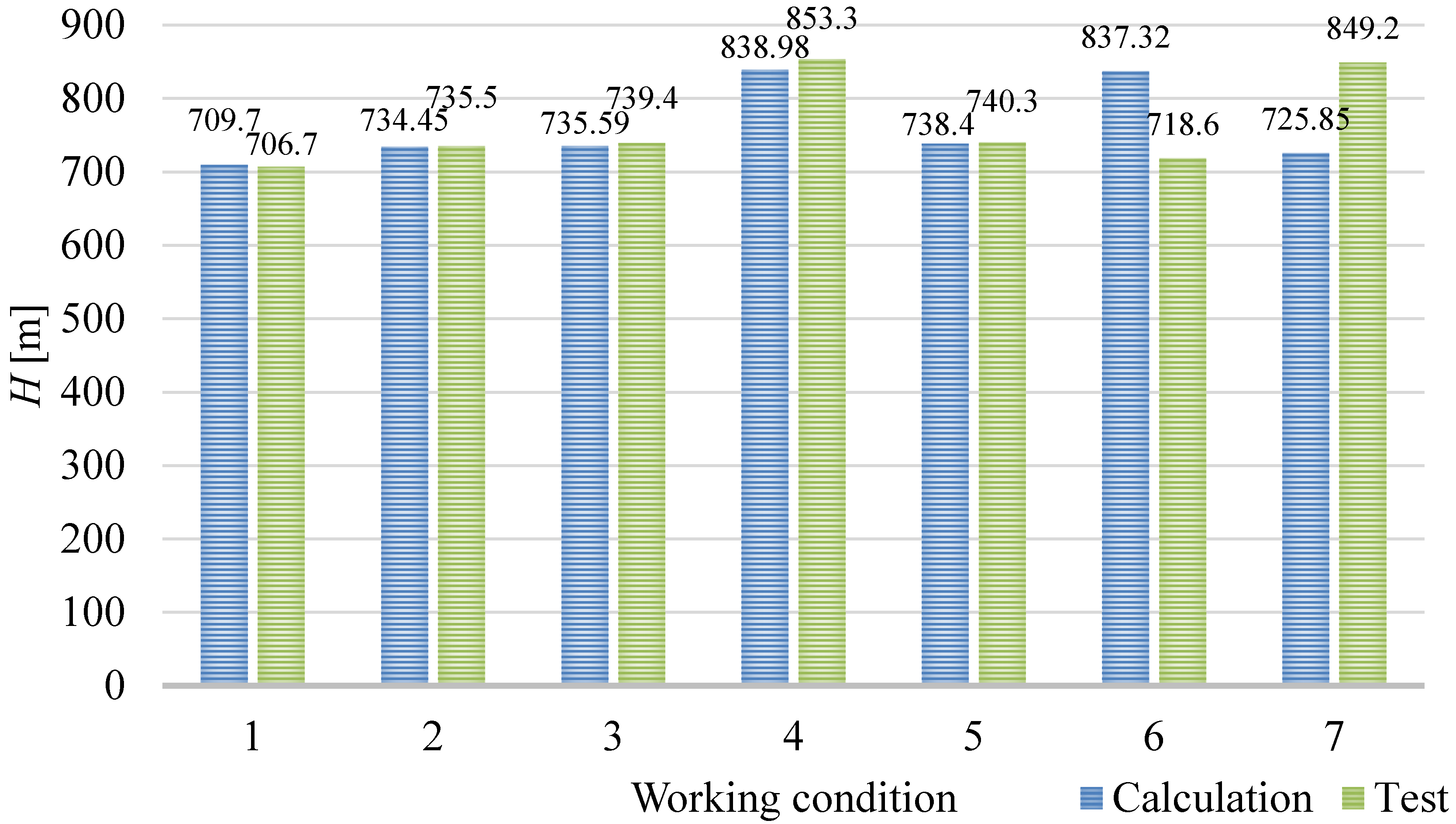
Under all 7 working conditions shown in Table 2, the calculation and test results are compared in Figure 3 in order to verify the settings’ feasibility. The test was carried out on the pump manufacturer’s test bench, and its comprehensive efficiency uncertainty was 0.2%. It can be seen that the calculated head is close to the test value with an error less than 10%, proving the calculation results credible.
3. Results and Discussion
3.1. Analysis of External Characteristics
The calculated external characteristic curve is shown in Figure 4, where Q, H, η, and M represent the flowrate, head, efficiency, and torque, respectively. The design point with the highest efficiency is at Q = 4500 m3/h, and the hump occurs at Q = 3600 m³/h which is 0.8 times the design flowrate. The top and bottom of the positive slope curve are called the peak and valley condition as shown in Figure 4.
The energy conversion relationship in the pump is shown in Figure 5, where P, M, ω, Qt, Ht, q, Q, h, and H represent the shaft power, shaft torque, rotational speed, theoretical flowrate, theoretical head, flowrate loss, actual flowrate, hydraulic loss, and actual head.
After the shaft power P compensates for the disc friction loss Pf, volume loss Pv, and hydraulic loss Ploss, the remaining part is just Pe, namely the effective output power of the pump.
Since the Pf and Pv are always much smaller than the Ploss, the following relationship can be obtained, approximately:
In this paper, the theoretical head Ht calculated by the impeller torque and rotational speed is used to represent the impeller input power. This calculation method bypasses the Euler head formula and thus has higher accuracy. The H is equal to the sum of the Ht and the total hydraulic loss h. If the hydraulic loss in the impeller, diffuser, and volute are recorded as h1, h2, h3, and it is agreed that the hydraulic loss is negative, the following relationship exists:
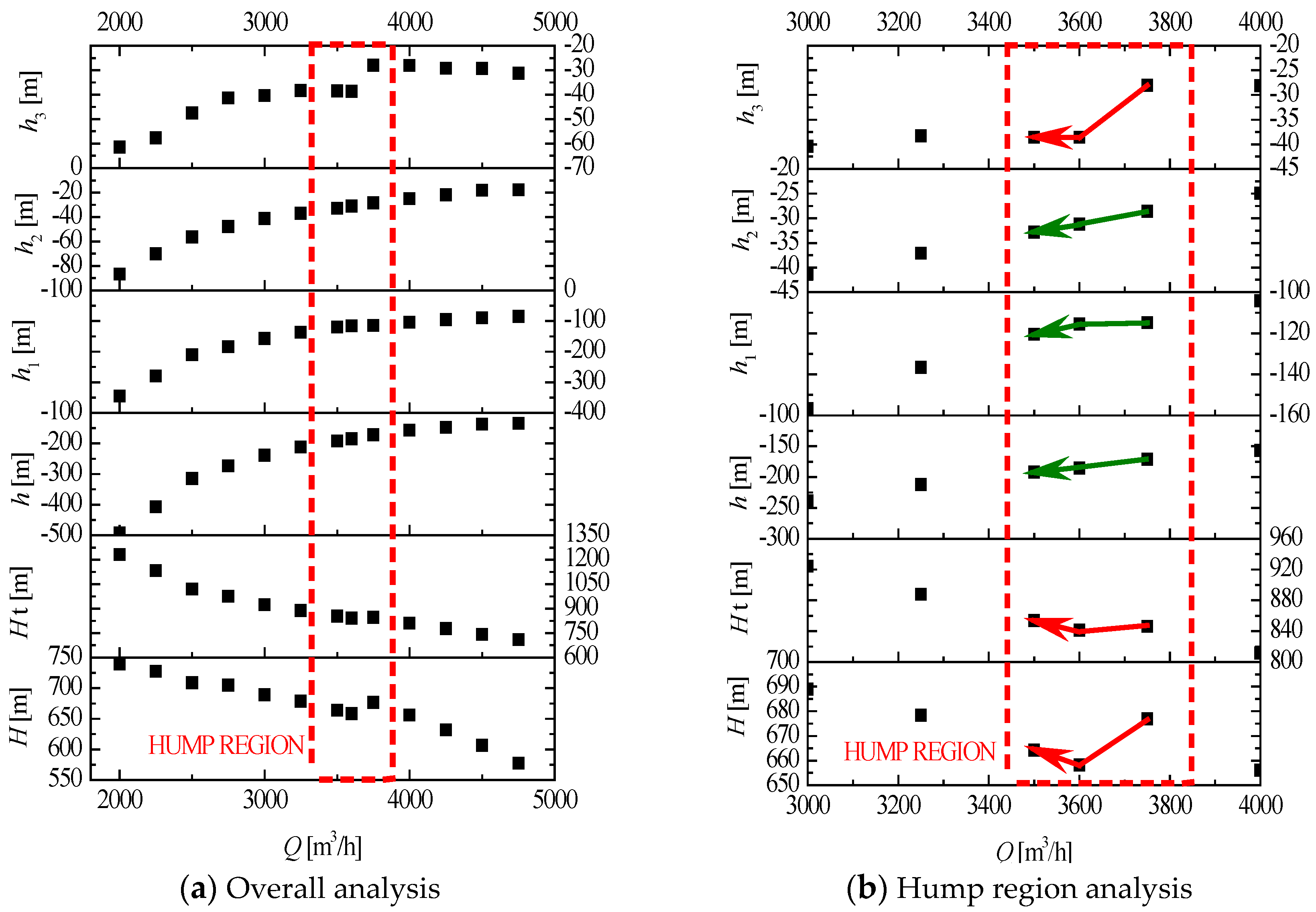
The Ht and the hydraulic loss distribution in the pump are shown in Figure 6a, and it can be seen that the Ht is much larger than the H, but their overall trends are nearly the same. Hydraulic loss h1 in the impeller is the largest among all components, and h3 in the volute is the smallest. Total hydraulic loss h and each component of hydraulic loss increase slowly as the flowrate decreases. The hump region highlighted in the red dashed box in Figure 6b shows that hump is formed by first the decrease and then the increase in the H, and the Ht experiences the same change trend, while the h changing trend varies little in the hump region. Among all components, h3 in the volute has the same changing trend as the H. It is concluded that the key factor leading to hump is the Ht, and h3 plays a small role.
The impeller capacity for work is mainly obtained by impeller blades agitating water, so it can be considered that the Ht is the sum of the theoretical head produced by all impeller blades. Under the peak and valley condition, the Ht produced by every impeller blade is displayed in Figure 7. Under the valley condition, the Ht of most blades is larger than that under the peak condition, except for the No. 6, 8, and 10 blades, whose Ht is lower. It can be seen that it is these three blades that cause the Ht to be lower under the valley condition than the peak condition. Here, these three blades are called abnormal blades. Next, the flow field and pressure field are analyzed to explain the reason for the abnormal blades’ formation, and reveal the hump formation mechanism.
3.2. Analysis of Changes in Impeller Capacity for Work
The external characteristic is the macroscopic manifestation of flow in the pump, so the hump formation mechanism can be revealed by analyzing the microscopic flow field. By comparing the flow pattern in the pump under the peak and valley condition, an obvious difference in the flow pattern is found in the diffuser. Figure 8 expands the internal flow field and pressure field in the diffuser in the cascade form, where 1 to 12 represent the diffuser blade number, and 0.1 to 0.9 represent different blade spans. Under the peak condition, the streamline is smooth, while with stall, namely large flow separation occurs under the valley condition, which destroys the rectification and pressurization function of the flow channel, causing apparent high pressure at the diffuser inlet. Stall cells have the effect of blocking the flow channel and greatly increasing the inlet pressure, which is called the blocking and pressurization effect.
The pressure distribution at the inlet and outlet of the diffuser and the flow pattern in the diffuser are both shown in Figure 9, where the red curve and red dotted line represent the circumferential pressure distribution and average pressure at the diffuser outlet, and the blue curve and blue dotted line correspond to the diffuser inlet. It can be seen from Figure 9 that under the peak condition, the diffuser works well with a smooth flow and regular pressure distribution at the inlet and outlet. Under the valley condition, the pressure distribution uniformity at both the inlet and outlet is destroyed by stall, and the inlet pressure near the flow passage where the stall cell exists increases significantly, marked by Pressure Rise in Figure 9. This is an intuitive manifestation of the blocking and pressurization effect of stall.
It is the blocking and pressurization effect of stall that cause the pressure rise at the diffuser inlet and impeller outlet, affecting the impeller capacity for work. The following takes the abnormal blade No. 6 in Figure 7 as an example to make a detailed analysis. The pressure distribution and capacity for work in the Ht of the No. 6 blade under the peak and valley conditions are compared in Table 3. Due to the blocking and pressurization effect of stall, the pressure on the blade outlet section is significantly increased from the peak to valley condition. However, the Ht distribution points out that from the peak to the trough, the Ht of the pressure side near the blade outlet rises little, while the of the suction side near the blade outlet rises much more. Because the Ht generated by the suction side is always negative, from the peak to valley condition, there is a decrease in the Ht of the whole No. 6 blade. After analyzing other abnormal blades in Figure 7, the same conclusion can be found. The reason that the blocking and pressurization effect of stall has a much greater influence on the impeller suction side than the pressure side is analyzed as follows.
On the impeller blade, the and dM produced per unit area have the following relationship:
where ρ, Q, and ω, respectively, represent the fluid density, volume flowrate, and rotational angular velocity. The relationship between the dM and blade angle α is shown in Figure 10a, so the can be further expressed as:
where dS represents the unit area on the impeller blade; R represents the distance from dS to the pump shaft; and P represents the static pressure on dS.
Affected by the blocking and pressurization effect of stall in the diffuser, the pressure on the impeller outlet section increases by the and the capacity for work changing range can be expressed as:
So, when the pressure rise produced by stall in the diffuser is imposed on the outlet section of both sides of the impeller blade, the on the side with a greater α must be greater than the other side. For the back-bend impeller blade, α on the suction side near the trailing edge is always larger than the pressure side as shown in Figure 10b. Therefore, the produced by stall forms larger on the suction side than the pressure side. This can also be clearly seen from the Ht distribution on the impeller blade as shown in Figure 10c. The position on the suction side with the largest is closer to the blade outlet than that on the pressure side. In conclusion, because α on the suction surface near the impeller outlet section is much larger than that on the pressure surface, the stall blocking and pressurization effect has a greater impact on the suction surface. The capacity for work of the two sides of the impeller blade is affected by the pressure rise to a different degree, and the Ht change in the whole blade is consistent with the blade suction side. Namely, from the peak to the valley condition, the sudden increase in the stall degree can cause the Ht of the impeller blades nearby to decrease; thereby, abnormal blades are formed. When there are too many severe abnormal blades, hump is formed.
3.3. Analysis of Volute Loss
The sudden increase in the volute hydraulic loss is a secondary factor in inducing hump, and its reason can be discussed by the loss analysis method based on the energy equation [12,13]. In the case of neglecting compressibility, temperature changes, and heat conduction, this method develops an energy balance formula, and the expression is shown in Equation (7):
In the formula, PL, μ, μt, k, and a’ represent the power loss, dynamic viscosity, eddy viscosity coefficient, turbulent kinetic energy, time average value, and pulsation value of physical quantity a, respectively. is the Kronecker Symbol (the function value is equal to 1 when i = j, and equal to 0 in other cases).
If the four terms on the right side of Equation (7) are called Term 1, Term 2, Term 3, and Term 4, then the Equation (7) can be simplified as:
The physical meanings of these four terms are “Reynolds stress work”, “viscous force work”, “the turbulent kinetic energy production”, and “the viscous dissipation”, respectively. Reynolds stress work and viscous force work cause the average kinetic energy diffusion. The turbulent kinetic energy production characterizes the energy converted into turbulent kinetic energy, and the viscous dissipation characterizes the energy directly converted into thermal energy.
By the loss analysis method, the internal loss composition and distribution of each component of the main feedwater water pump can be obtained as shown in Figure 11, where the ordinate adopts a logarithmic form to compare the total power loss of the four terms in the volute under the peak and valley conditions. It can be seen that Term 2 and Term 4 are so small that they can be ignored, and power loss in the volute is mainly caused by the turbulent kinetic energy production of Term 3, followed by Reynolds stress work of Term 1. During the process from the peak to valley condition, Term 3 surges from 5008.51 W to 20660.7 W with an increase of 313%, and Term 1 rushes from 1696.33 W to 6651.78 W with an increase of 292%.
The distribution of Term 1 and Term 4, and the flow pattern in the volute are shown in Table 4. Under the peak condition, there is a symmetrical vortex pair in the cross section of volute passage, and the flow velocity is higher between the two vortices and near the diffuser outlet jet. In the district where high and low velocity flow contact, both Term 1 and Term 3 produce a large value. However, under the valley condition, the vortex pair in the volute cross section has a poor symmetry, and the high-velocity area between the two vortices is larger than that under the peak condition. Besides, the diffuser outlet jet extends downstream much to form a larger high-velocity area. As known from the above analysis, Term 1 and Term 3 produce a larger value at the junction of the high and low velocity area. Because the high-speed area in the volute under the trough condition is larger, and thus the high-low-speed contact area is larger as well, the Term 1 and Term 3 values are much larger than those under the peak condition.
It can be seen that during the process from the peak to valley condition, the diffuser outlet jet aggravates, and the flow asymmetry and turbulence degree in the volute increase much. Thus, the loss caused by Reynolds stress work and turbulent kinetic energy production increases severely so that the volute hydraulic loss increases sharply from the peak to valley condition.
4. Conclusions
The hump analysis process is rigorous and precise with little uncertainty. The uncertainty in this paper mainly comes from the experiment and simulation. The test results are obtained by a test platform with a comprehensive efficiency uncertainty of 0.2%, ensuring that the test uncertainty is extremely small. By comparing with the test, the calculation error is within 10%. Therefore, the uncertainty of the test and simulation is small, and its influence on the research is little. The head curve hump formation mechanism of the main feedwater pump is analyzed, and the following conclusions can be drawn:
- (1)
- Along the direction of the flowrate decrease, the pump head curve suddenly drops to form a hump at a small flowrate. The main external characteristic factor causing hump is the sudden Ht drop, followed by the sudden hydraulic loss increase in the volute;
- (2)
- From the hump peak to valley, the flow pattern in diffuser changes from a smooth style to stall. Stall cells have the effect of blocking and pressurization, resulting in a Ht decrease on impeller blades. When the impeller blades are affected by stall to a relatively high degree, Ht of the whole impeller decreases;
- (3)
- The diffuser stall blocking and pressurization effect causes a Ht increase on the impeller blade pressure side, and a Ht decrease on the blade suction side. Because the blade angle of the suction side near the trailing edge is much larger than the blade angle of the pressure side, the Ht descent range on the suction side is greater than the Ht rise range on the pressure side. Thus, diffuser stall can cause the Ht drop of the whole blade and even the whole impeller;
- (4)
- From the hump peak to valley, the diffuser outlet jet aggravates, and the flow asymmetry and turbulence degree in the volute increase much. Then, the loss caused by Reynolds stress work and turbulent kinetic energy production increases severely so that the volute hydraulic loss increases sharply from the peak to valley condition.
The latest research on the pump hump believes that the Ht change is the main reason for the hump formation, and it is found that the Ht change is basically synchronized with the appearance of diffuser stall, but the detailed mechanism of how stall induces hump is not explained yet [12,19,20]. This is exactly the problem that this article focuses on. It is believed that this article will help to understand the hump formation mechanism more deeply and provide a valuable reference for suppressing hump.
Author Contributions
Y.L.: experiment, simulation, and analysis; D.W.: supervision; H.R.: data curation; R.X.: article writing; Y.S.: CFX post-processing; B.G.: mesh generation. All authors have read and agreed to the published version of the manuscript.
Funding
This research received no external funding.
Institutional Review Board Statement
Not applicable.
Informed Consent Statement
Not applicable.
Conflicts of Interest
The authors declare that they have no known competing financial interests or personal relationships that could have appeared to influence the work reported in this paper.
Nomenclature
| Parameter | Symbol | Parameter | Symbol |
| head | H | theoretical head | Ht |
| flowrate | Q | hydraulic loss | h |
| torque | M | blade angle | α |
| efficiency | η | impeller rotation speed | ω |
| power | P |
References
- Zhao, X. Numerical Analysis and Mechanical Research of Main Feedwaterwater (Pressure) Pump for Ling’ao Ⅱ Nuclear Power Station. Ph.D. Thesis, Shanghai Jiaotong University, Shanghai, China, 2015. [Google Scholar]
- Li, D.; Chang, H.; Zuo, Z.; Wang, H.; Li, Z.; Wei, X. Experimental investigation of hysteresis on pump performance characteristics of a model pump-turbine with different guide vane openings. Renew. Energy 2020, 149, 652–663. [Google Scholar] [CrossRef]
- Sampedro, E.O.; Dazin, A.; Colas, F.; Roussette, O.; Coutier-Delgosha, O.; Caignaert, G. Multistage radial flow pump-turbine for compressed air energy storage: Experimental analysis and modeling. Appl. Energy 2021, 289, 116705. [Google Scholar] [CrossRef]
- Gülich, J.F. Centrifugal Pumps; Springer: Berlin/Heidelberg, Germany, 2008. [Google Scholar]
- Zhou, P. Investigation of Stall Characteristics in Centrifugal Pumps. Ph.D. Thesis, China Agricultural University, Beijing, China, 2015. [Google Scholar]
- Xiao, Y.; Yao, Y.; Wang, Z.; Luo, Y.; Zeng, C.; Zhu, W. Hydrodynamic mechanism analysis of the pump hump district for a pump-turbine. Eng. Comput. 2016, 33. [Google Scholar] [CrossRef]
- Ye, W.; Ikuta, A.; Chen, Y.; Miyagawa, K.; Luo, X. Numerical simulation on role of the rotating stall on the hump characteristic in a mixed flow pump using modified partially averaged Navier-Stokes model. Renew. Energy 2020, 166, 91–107. [Google Scholar] [CrossRef]
- Yang, J. Flow Patterns Causing Saddle Instability in the Performance Curve of a Centrifugal Pump with Vaned Diffuser. Ph.D. Thesis, Jiangsu University, Zhenjiang, China, 2014. [Google Scholar]
- Fisher, R.K.; Webb, D.R. Effect of Cavitation on the Discontinuity Point and On Alternating Pressures and Gate Torques on a Pump/Turbine Model In The Pump Cycle; Allis-Chalmers Corporation, Hydro-Turbine Division: West Allis, WI, USA, 1978. [Google Scholar]
- Braun, O.; Kueny, J.L.; Avellan, F. Numerical analysis of flow phenomena related to the unstable energy-discharge characteristic of a pump-turbine in pump mode. In Proceedings of the ASME 2005 Fluids Engineering Division Summer Meeting, Houston, TX, USA, 19–23 June 2005; American Society of Mechanical Engineers: New York, NY, USA, 2005; pp. 1075–1080. [Google Scholar]
- Gentner, C.; Sallaberger, M.; Widmer, C.; Braun, O.; Staubli, T. Numerical and experimental analysis of instability phenomena in pump turbines. IOP Conf. Ser. Earth Environ. Sci. 2012, 15, 032042. [Google Scholar] [CrossRef]
- Sun, Y.K. Instability Characteristics and Influencing Factors of Positive Slope on Pump Performance Curves of a Low-Specific-Speed Pump-Turbine. Ph.D. Thesis, Tsinghua University, Beijing, China, 2016. [Google Scholar]
- Ran, H.; Liu, Y.; Luo, X.; Shi, T.; Xu, Y.; Chen, Y.; Wang, D. Experimental comparison of two different positive slopes in one single pump-turbine. Renew. Energy 2020, 154, 1218–1228. [Google Scholar] [CrossRef]
- Ran, H.; Luo, X. Experimental study of instability characteristics in pump-turbine. J. Hydraul. Res. 2018, 56, 871–876. [Google Scholar] [CrossRef]
- Erne, S.; Edinger, G.; Maly, A.; Bauer, C. Simulation and experimental investigation of the stay vane channel flow in a reversible pump turbine at off-design conditions. Period. Polytech. Mech. Eng. 2017, 61, 94–106. [Google Scholar] [CrossRef] [Green Version]
- Naterer, G.; Camberos, J. Entropy-Based Design and Analysis of Fluids Engineering Systems; CRC Press: Boca Raton, FL, USA, 2008. [Google Scholar]
- Li, D.; Gong, R.; Wang, H.; Xiang, G.; Wei, X.; Qin, D. Entropy production analysis for hump characteristics of a pump turbine model. Chin. J. Mech. Eng. 2016, 29, 803–812. [Google Scholar] [CrossRef]
- Wilhelm, S.; Balarac, G.; Métais, O.; Ségoufin, C. Analysis of head losses in a turbine draft tube by means of 3D unsteady simulations. Flow Turbulence Combust. 2016, 97, 1255–1280. [Google Scholar] [CrossRef] [Green Version]
- Lu, G. Investigations on the Influence of the Flow Separation in Guide Vane Channels on the Positive Slope on the Pump Performance Curve in a Pump-Turbine. Ph.D. Thesis, Tsinghua University, Beijing, China, 2018. [Google Scholar]
- Lu, G.; Zuo, Z.; Liu, D.; Liu, S. Energy balance and local unsteady loss analysis of flows in a low specific speed model pump-turbine in the positive slope region on the pump performance curve. Energies 2019, 12, 1829. [Google Scholar] [CrossRef] [Green Version]
- Li, D. Investigation on Flow Mechanism and Transient Characteristics in Hump Region of a Pump-Turbine. Ph.D. Thesis, Harbin Institute of Technology, Harbin, China, 2017. [Google Scholar]
- Luo, T. Fluid Mechanics; China Machine Press: Beijing, China, 2007. [Google Scholar]
- Cravero, C.; Marsano, D. Criteria for the stability limit prediction of high-speed centrifugal compressors with vaneless diffuser. Part I: Flow structure analysis. In Proceedings of the ASME Turbo Expo 2020: Turbomachinery Technical Conference and Exposition, Virtual Conference, 21–25 September 2020. ASME Paper GT2020-14579. [Google Scholar]
- Cravero, C.; Marsano, D. Criteria for the stability limit prediction of high-speed centrifugal compressors with vaneless diffuser. Part II: The development of prediction criteria. In Proceedings of the ASME Turbo Expo 2020: Turbomachinery Technical Conference and Exposition, Virtual Conference, 21–25 September 2020. ASME Paper GT2020-14589. [Google Scholar]
Figure 1.
Pump model and mesh: (a) annular suction chamber, (b) impeller, (c) diffuser, (d) volute.

Figure 2.
Real impeller.

Figure 3.
Calculation feasibility verification.

Figure 4.
External characteristic curve.

Figure 5.
Energy conversion relationship in the main feedwater pump.

Figure 6.
Analysis of Ht and hydraulic loss.

Figure 7.
Distribution of impeller blade capacity for work.

Figure 8.
Flow field comparison in diffuser under peak and valley condition.


Figure 9.
Blocking and pressurization effect of stall in the diffuser.

Figure 10.
Analysis of blade capacity for work.

Figure 11.
The power loss composition in volute under the peak and valley condition.


Table 1.
The main design and performance parameters (pump mode, design point).
| Parameter | Symbol | Value |
|---|---|---|
| Number of impeller blades | Zi | 2 × 5 |
| Impeller inlet diameter | D1 | 276 mm |
| Impeller outlet diameter | D2 | 484 mm |
| Impeller blade outlet width | b2 | 71 mm |
| Blade angle at impeller outlet | β2 | 24° |
| Impeller blade wrap angle | φ | 142° |
| Vaneless zone gap | δ | 12.5 mm |
| Blade height of diffuser | b3 | 72 mm |
| Blade number of diffuser | Zd | 12 |
Table 2.
Main operating parameters.
| Operating Condition | Medium | Temperature (°C) | Pressure (bar) | Flowrate (m3/h) | Rotational Speed (rpm) |
|---|---|---|---|---|---|
| 1 | water | 184.1 | 11.01 | 3762 | 5080 |
| 2 | 183 | 10.73 | 3674 | 5131 | |
| 3 | 184.1 | 11.01 | 3585 | 5115 | |
| 4 | 183 | 10.73 | 3501 | 5399 | |
| 5 | 184.1 | 11.01 | 3658 | 5139 | |
| 6 | 183 | 10.73 | 3572 | 5407 | |
| 7 | 184.1 | 11.01 | 3893 | 5155 |
Table 3.
Comparison of the capacity for work of the No. 6 blade.
| Pressure Distribution | Ht Distribution | |||
|---|---|---|---|---|
| Pressure Side | Suction Side | Pressure Side | Suction Side | |
| Peak |  |  |  |  |
| Valley |  |  |  |  |
| Legend |  |  |  |  |
Table 4.
The flow pattern and power loss distribution in volute under hump condition.
| Streamline | Term1 | Term3 | |
|---|---|---|---|
| Peak |  |  |  |
| Valley |  |  |  |
| Legend |  |  |  |
Publisher’s Note: MDPI stays neutral with regard to jurisdictional claims in published maps and institutional affiliations. |
© 2021 by the authors. Licensee MDPI, Basel, Switzerland. This article is an open access article distributed under the terms and conditions of the Creative Commons Attribution (CC BY) license (https://creativecommons.org/licenses/by/4.0/).
Share and Cite
MDPI and ACS Style
Liu, Y.; Wang, D.; Ran, H.; Xu, R.; Song, Y.; Gong, B. RANS CFD Analysis of Hump Formation Mechanism in Double-Suction Centrifugal Pump under Part Load Condition. Energies 2021, 14, 6815. https://doi.org/10.3390/en14206815
AMA Style
Liu Y, Wang D, Ran H, Xu R, Song Y, Gong B. RANS CFD Analysis of Hump Formation Mechanism in Double-Suction Centrifugal Pump under Part Load Condition. Energies. 2021; 14(20):6815. https://doi.org/10.3390/en14206815
Chicago/Turabian StyleLiu, Yong, Dezhong Wang, Hongjuan Ran, Rui Xu, Yu Song, and Bo Gong. 2021. "RANS CFD Analysis of Hump Formation Mechanism in Double-Suction Centrifugal Pump under Part Load Condition" Energies 14, no. 20: 6815. https://doi.org/10.3390/en14206815
Note that from the first issue of 2016, this journal uses article numbers instead of page numbers. See further details here.