Article

Root System Analysis and Influence of Moisture on Soil Electrical Properties

by
Antonio M. Silva Filho
1,2,3,*,
José R. S. Silva
2,
Glaciano M. Fernandes
2,
Lucas D. S. Morais
2,
Antonio P. Coimbra
4 and
Wesley P. Calixto
1,2,*
1
Electrical, Mechanical & Computer Engineering School (EMC), Federal University of Goias (UFG), Goiania 74605-010, GO, Brazil
2
Studies and Researches in Science and Technology Group, Federal Institute of Goias (IFG), Senador Canedo 75250-000, GO, Brazil
3
Federal Institute of Tocantins (IFTO), Palmas 77020-450, TO, Brazil
4
Institute of Systems and Robotics, University of Coimbra, 3030-290 Coimbra, Portugal
*
Authors to whom correspondence should be addressed.
Energies 2021, 14(21), 6951; https://doi.org/10.3390/en14216951
Submission received: 16 September 2021 / Revised: 6 October 2021 / Accepted: 9 October 2021 / Published: 22 October 2021

Abstract

:
This paper proposes a methodology for plant root system and soil moisture analysis through the geoelectrical prospecting method. Overall, bench and field experiments are implemented to analyze the behavior of electrical conductivity of the soil in relation to moisture content and plant root system growth. Specifically, Wenner array and lateral profiling technique are used to stratify the soil in horizontal layers, performing in-depth analysis. Millet (Pennisetum glaucum L.), bean (Phaseolus vulgaris L.) and sorghum (Sorghum bicolor L. Moench) are used to analyze the root system behavior. Results show that the soil water dynamics can be observed through soil stratification in horizontal layers and the plant root system is correlated with apparent electrical conductivity of the soil. Thus, geoelectric prospecting methods can be used as an analysis tool, both of soil moisture dynamics and of plant roots, to support decision making regarding soil and crop management.

1. Introduction

Apparent electrical conductivity of the soil σ a describes the soil’s ability to conduct electric current. Overall, a field experiment is conducted using an electric current apparatus to apply an electric current I to the ground and measure a resulting voltage V, which allows the calculation of σ a values [1]. The apparent conductivity of the soil σ a varies according to physico-chemical properties contained in soil under study. Mapping σ a is, therefore, an efficient tool in the investigation of soil behavior and spatial variability, allowing the identification of areas with similar properties and delimiting differentiated management units [2,3].
With this knowledge, the inputs insertion locations into the soil can be managed before planting. In the literature there are several works developed with the focus on understanding σ a for inputs application in planting. Moral, Terrón and Marques [4] use multivariate geostatistics associated with σ a data to obtain soil properties to determine management zones. Before planting, 70 soil samples at 20 cm depth are collected and georeferenced in an area of 33 ha. The survey of σ a is carried out using a commercial geoelectric instrument for direct contact measurement, operating in shallow (0 cm–30 cm) and deep (0 cm–90 cm) modes. The σ a values have high correlation with soil texture, cation exchange capacity (CEC), organic matter and nitrogen content, demonstrating that σ a mapping is a fast and low-cost tool to obtain information. In addition, σ a data are related to soil fertility parameters and therefore, conductivity can be used to delimit management zones.
Johnson et al. [5] evaluate σ a use on a field scale to identify soil characteristics related to productivity and ecological properties in wheat, corn and millet crops. The σ a mapping is carried out in a region of 250 ha at 30 cm depth. Physical, chemical and biological parameters are correlated with σ a , which allows the application of electrical conductivity mapping to obtain spatial data for productivity and soil condition.
Serrano, Shahidian and Marques [6] evaluate spatial and temporal dynamics of σ a measured in a 6 ha pasture field using electromagnetic induction sensor, over seven years. Through 76 georeferenced samples, the soil is characterized in terms of texture, moisture content, pH, organic matter content, nitrogen, phosphorus and potassium. Thus, significant correlations are obtained among σ a and the relative elevation of the field, pH, silt and soil moisture content, allowing identification of areas with similar characteristics for which the same type of management can be recommended.
Analysis of σ a for mapping the spatial variability of soil properties using a reduced number of samples is analyzed by Sanches et al. [7]. The traditional high-density sampling process is applied experimentally in sugar cane field, in addition to electric conductivity measurement by a direct contact sensor. Method application obtains maps of acceptable precision used to formulate recommendations for limestone application. Collection process guided by σ a mapping resulted in 20 sampling points and suggested application of 28 tons of lime, similar to the value of 30 tons obtained based on the high-density collection process that, on the other hand, included 204 sampling points. The survey of the electrical conductivity of the soil in field allows the implementation of reduced and targeted sampling, which makes the collection process less financially costly.
Regarding soil management using σ a previous to planting, there are several mapping techniques; however, soil analysis using σ a after planting is poorly described in the literature. For soil mapping after planting, Shi, Webster and Triantafilis [8] analyzes the relationship between σ a and soil salinity in rice cultivation. Through three-dimensional mapping of electrical conductivity of the soil, salinity spots are identified consistent with reduction in crop productivity yield of approximately 33% in the region indicated by high salinity. Relationship between σ a and rice production pattern presents the potential of this approach for soil management through monitoring salinity.
Corwin et al. [9] demonstrate how σ a spatial distribution can guide collecting soil samples process to determine the properties that influence cotton planting yield. Cotton yield response model is developed based on regression analysis of ordinary minimum squares and adjusted for spatial autocorrelation using maximum verisimilitude. Measurement of σ a is influenced by soil properties that also influence cotton productivity. Consequently, by knowing soil properties that affect crop yield, recommendations can be performed to improve productivity.
Three-year historical production maps in conjunction with σ a mapping are used by Cillis et al. [10] to determine homogeneous zones. Analysis is conducted using electrical conductivity, characteristics related to soil upper portion (0 cm–50 cm) and related to the roots of corn (Zea mays L.), soybean [Glycine max (L.) Merr.] and wheat (Triticum aestivum L.). Therefore, correlation among texture, organic matter and soil salinity with electrical conductivity, indicates σ a use as a tool for studying and managing changes in soil fertility.
Geoelectric methods use in soil sciences, with emphasis on root architecture delineation is analyzed by Cimpoiaşu et al. [11]. Geoelectric methods offer non-invasive data acquisition, with low cost and have the capacity for space-time monitoring of the main physical, chemical and biological processes in plants root system ( R S ) zone. R S performs functions of fixation in the soil, absorption of water and nutrients [11,12,13]. Soil electrical conductivity values are quantitatively associated with root mass, making it possible to evaluate and quantify roots distribution in the soil through geoelectric methods [11,12,13,14,15]. Roots affect soil electrical conductivity in the same order of magnitude as the effects caused by other soil properties, such as moisture and texture, for example [12,14].
Understanding the growth dynamics of plants R S is as important as knowing soil properties. In other words, studies to assess distribution, volume and root mass are fundamental for improving fertilization, localized irrigation and subsoiling. Despite the importance for agricultural management, there is a lack of data on plants R S due to methodological difficulties inherent to roots growth dynamics. Soil is the opaque cultivation medium for R S and therefore, makes it difficult to observe the roots. Another problem is that destructive methods involving soil excavating to expose the roots have the disadvantage of causing damage to plants and soil [14].
Thus, this paper aims to evaluate the relationship between R S in the soil and apparent electrical conductivity σ a values through geoelectric prospecting method in laboratory and field experiments. The originality of proposed study is R S analysis at three different depths to verify roots behavior not only on surface. Field study uses the lateral profiling technique for electrodes arrangement in the soil in crops of millet, sorghum, beans and uncultivated area for comparison purposes. Horizontal and vertical soil stratification is an innovative analysis, as it allows σ a measurement at greater soil depths.
Methods based on electric current injection in the soil can be applied in field without the need to modify the edaphic environment. Geoelectric prospecting methods, in addition to simplicity and low cost, can be applied on a larger scale than invasive methods. Furthermore, geoelectric methods are non-invasive and, consequently, σ a measurements can be repeated for plants R S analysis including at different depths to provide a reliable assessment of the distribution, volume and root mass [14,15].
This work is structured as: Section 2 provides a brief description of soil moisture and compaction, stratification methods and plants root system ( R S ). Section 3 presents the proposed methodology for laboratory and field studies, Section 4 presents the results obtained from the application of proposed methodology and Section 6 the conclusion of this paper.

2. Theoretical Background

This section briefly presents moisture and soil compaction concepts, since these properties directly affect plants development and presents the correlation of these concepts with electrical conductivity of the soil σ a . Additionally, this section describes σ a survey process for soil stratification in horizontal layers and R S definitions.

2.1. Moisture and Soil Compaction

Soil moisture content ω corresponds to water portion contained in porous spaces of the soil, as illustrated in Figure 1. The ω values obtained in laboratory are given as a percentage of dry soil mass, resulting from the drying process in an oven at 110 °C between 12 h and 24 h [16]. In field measurements, time domain Reflectometry (TDR) meters are used, based on voltage pulse propagation time in a metal probe inserted in the ground [2].
Soil compaction C represents an increase in soil density and a consequent porosity reduction due to solid particles rearrangement. Soil is considered agronomically compacted when the proportion of total pore volume to soil volume is inadequate for crop development, causing for example nutritional deficiencies and decreased plant height. In addition, the formation of an impermeable layer can occur in compacted soils, which makes it difficult for water to infiltrate plants R S [17]. Both moisture and soil compaction are positively correlated with the apparent electrical conductivity of the soil σ a . However, σ a increases more with increasing moisture than with increasing compaction [3,18,19].

2.2. Soil Stratification Method

Electrical conductivity σ a is influenced by several soil factors such as porosity, dissolved electrolyte concentration, texture, organic matter, moisture content and compaction [20]. Figure 1 illustrates the three main electric current paths in the soil, in which the first path (in red) runs mainly through salt content in the water that occupies the largest pores. The second electric current path (red in color) travels through the solid phase in moist soils, mainly by exchangeable cations associated with the clay mineral. The third electric current path in the ground (red in color) travels through particles in direct and continuous contact with each other. The electrical conductivity that includes the combined effects of these three paths is defined as apparent electrical conductivity of the soil σ a [21]. Electric current path in yellow illustrated in Figure 1 is the representation for homogeneous soil.
Apparent electrical conductivity of the soil values is obtained by direct contact measurement finding the electric resistance or by indirect means using electromagnetic induction [4,6,7,22,23]. Obtaining by direct contact occurs by measuring apparent electrical resistance of the soil R m .
Thus, Wenner array is used, which the soil resistivity measuring instrument injects electric current into the ground and measures the voltage, as illustrated in Figure 1. The Wenner array is an electrical geoprospecting method based on Maxwell’s equations for electromagnetism. Soil resistivity meter in Figure 1 has four terminals, connected to four nailed rods aligned in the ground at depth P, and separated by distance a. Electric current I is injected and collected in the rods positioned at both ends, which produces electric potential V in intermediate rods. This potential difference Δ V of the inners electrodes is calculated by [1,23]:
Δ V = ρ I 4 π 1 a + 2 a 2 + ( 2 P ) 2 2 ( 2 a ) 2 + ( 2 P ) 2
Therefore, apparent electrical resistance R m is calculated from I and Δ V data through (2) [1,23]:
R m = Δ V I = ρ 4 π 1 a + 2 a 2 + ( 2 P ) 2 2 ( 2 a ) 2 + ( 2 P ) 2
Rearranging (2), the expression for calculating the apparent electrical resistivity of the soil ρ a [ Ω m ] for Wenner array is given by [23]:
ρ a ( a ) = 4 π a R m 1 + 2 a a 2 + ( 2 P ) 2 2 a ( 2 a ) 2 + ( 2 P ) 2
With ρ a , σ a can be find by calculating the inverse of ρ a . Based on ρ a ( a ) curve, in which a is the spacing between rods, several mathematical models were developed to stratify the soil in horizontal layers, each one with its own peculiarity. The expression used to horizontally stratify the soil with two layers using the Wenner array can be determined by rearranging (3), obtaining: [23]:
ρ a ( a ) = ρ 1 1 + 4 i = 1 K i 1 + ( 2 i · h 1 a ) 2 K i 4 + ( 2 i · h 1 a ) 2
in which i is the summation variable and K is given by:
K = ρ 2 ρ 1 ρ 2 + ρ 1
where ρ 1 and ρ 2 are the apparent resistivity of the first and second soil layers, respectively. Traditionally, stratification methods for layers number greater than two were developed based on the expression (4) of the apparent resistivity for soils with two layers [24]. Of the several known methods, can be mentioned the Pirson method [25], developed from the hypothesis that at each inflection point p f of the curve formed by the function ρ a ( a ) arises a new layer of soil. This hypothesis assumes the curve decomposition into increasing and decreasing sections and each section corresponds to two layers. So, an inflection point on the curve adds another layer.
Thus, found ρ a ( a ) , soil can be represented in horizontal layers, with the three-layer model being the most suitable, as it represents the soil profile in a more realistic way [26]. In precision agriculture, the characteristics related to the upper portion of the soil are evaluated, representing the soil layer thickness used by crops roots [7,10].

2.3. Lateral Profiling Method

Lateral profiling method consists of relocating the Wenner array electrodes at points following each separation, maintaining a fixed distance between rods. This methodology is used to obtain the horizontal mapping of ρ a . Figure 2 illustrates the method applied in Column 1 in A1, B1, C1 and D1. Horizontal mapping is obtained by tracing the other columns (Column 2, Column 3 and Column 4) [3,27]. The red circumference shown in Figure 2 indicates the measurement/stratification location.

2.4. Root System

Root system ( R S ) of plants includes the root, soil, water and air necessary for growth. The interactions between root characteristics and soil physical and chemical properties directly influence root growth and, consequently, the overall plant development [13,28].
The R S analysis methods are divided into destructive, non-destructive and non-invasive. Destructive methods implement soil excavation, while non-destructive methods use invasive devices to verify root growth without the need for excavation. Non-invasive methods, such as geoelectric methods, assess roots indirectly with little contact with the soil and the R S [13,29].
Geoelectric methods used in the analysis of R S obtain σ a values on the soil surface, i.e., approximately 10 cm depth. Thus, most in situ roots studies highlight the water dynamics exhibited by agricultural crops. In this type of environment, it is difficult to separate the effect of rootless soil [11]. Hence, the need for laboratory studies to analyze the localized behavior of the root zone and, consequently, support field tests. In general, σ a values in the field are obtained by direct contact methods (electrical resistance), with the dipole-dipole array being the most commonly used [11].

3. Methodology

This section presents the methodology used to analyze the correlation between R S of plants and apparent electrical conductivity of the soil σ a . Methodology to analyze moisture influence on σ a values is also presented, in which the proposed experimental procedure includes laboratory and field studies, as illustrated in Figure 3.

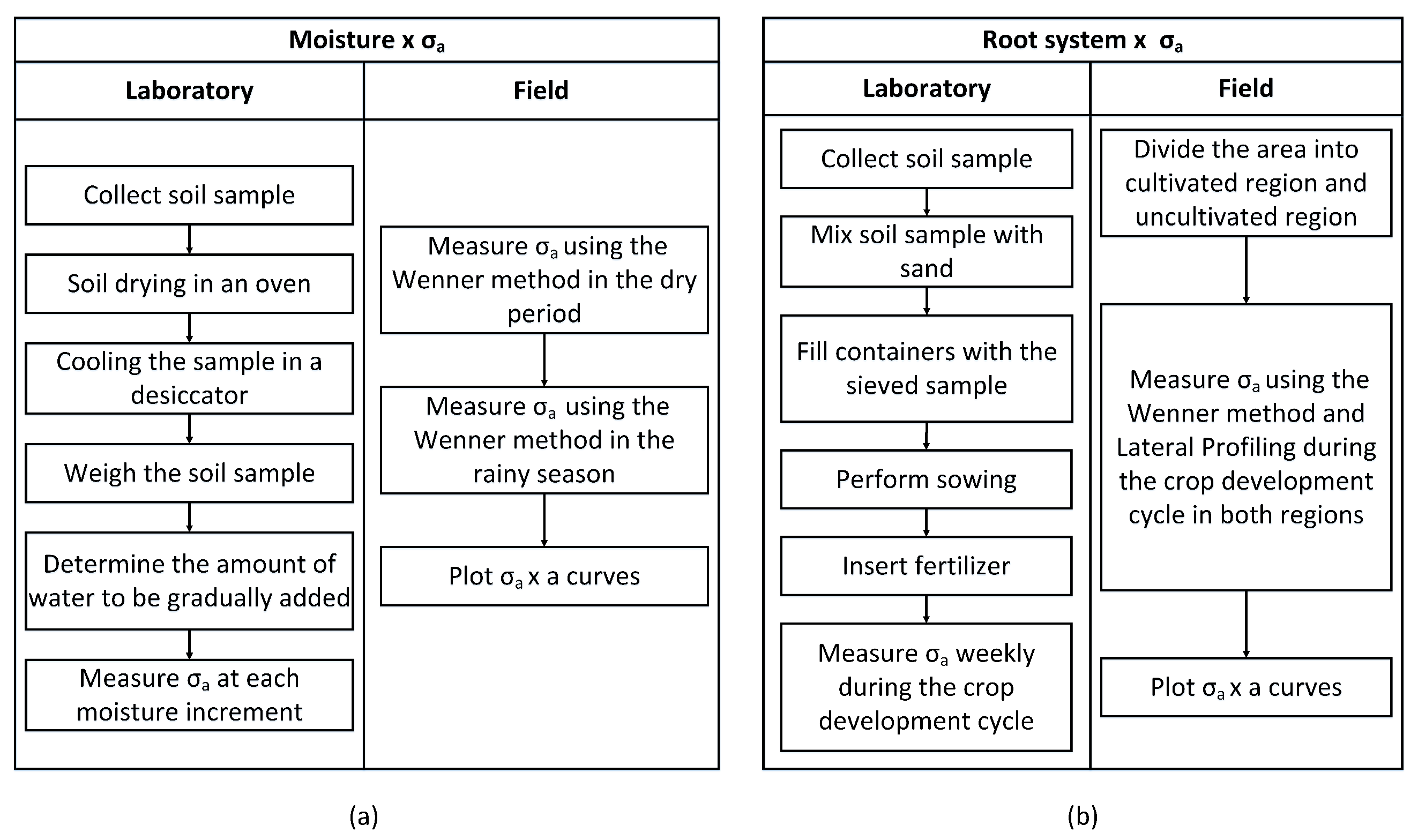
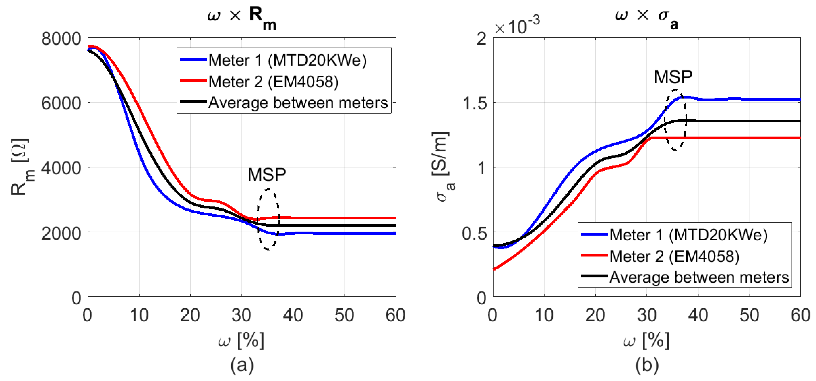
3.1. Relationship between Moisture × Electrical Conductivity of the Soil

The construction of a cylindrical container made of polyvinyl chloride (PVC) is required to relate moisture ω and apparent electrical conductivity of the soil σ a in laboratory experiment, as illustrated in Figure 3a. This container must contain inner radius r v c , wall thickness e v c and height L v c (Figure 4).
The container must have four holes with spacing a (Figure 4) for insertion of current and potential electrodes. After being collected, the soil sample is placed in the oven at 110 °C for a 24-h period, for moisture reduction. The aim is to obtain ω 0 . Afterwards, sample must remain for 24 h in the desiccator for cooling and to avoid absorbing moisture from the environment. Then, the sample cooled and with ω 0 must be inserted into the containers. Thus, the moisture content of the sample is gradually varied in intervals of ω = 5 % . At each increment in ω , the electrical resistance R m of the soil is measured using the apparent soil resistance meter, to obtain ω × σ a curve, using (3).
To measure the relationship between ω × σ a in the field, as illustrated in Figure 3a, it is necessary to find the apparent electrical resistivity of the soil ρ a , applying the Wenner array in A, B, C, 1, 2 and 3 directions, as illustrated in Figure 5. With ρ a × a curves and expressions (4) and (5), the stratified soil model in horizontal layers can be obtained. Spacing a values in the Wenner array are defined according to the experiment area.
As the purpose is to verify the relationship between ω × σ a , measurements are carried out both in dry and rainy season. The values shown are: (i) the mean for each direction of Wenner method application (Figure 5) and (ii) monthly values in the period under analysis.

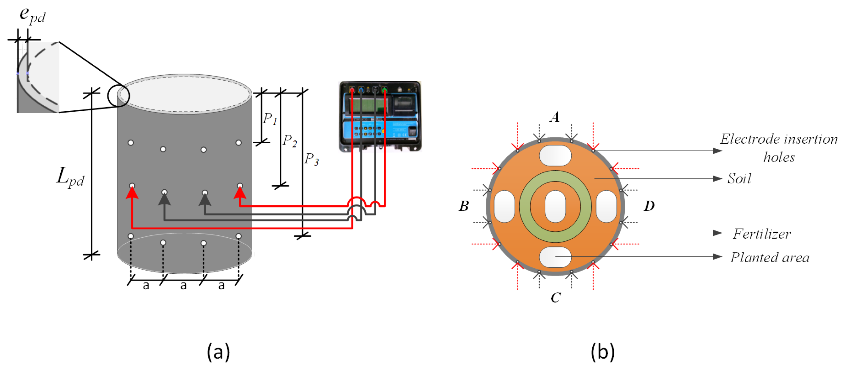
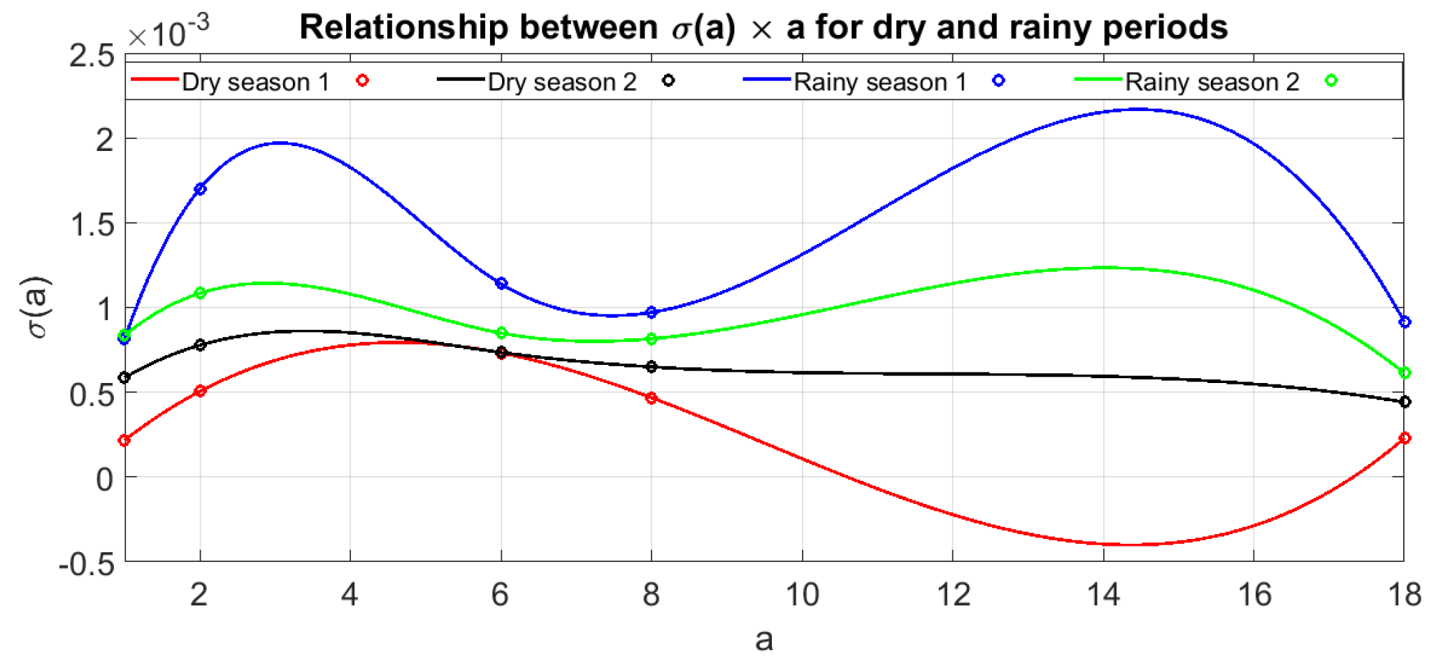
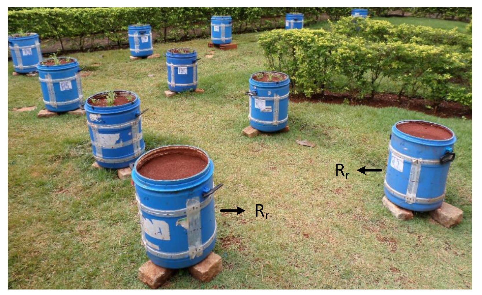
3.2. Relationship between Root System × Soil Electrical Conductivity

In laboratory, to apply the proposed methodology illustrated in Figure 3b and measure the relationship between R S and σ a , high-density polyethylene (HDPE) cylindrical containers required (Figure 6). The soil electrical resistance values R m are obtained through geoelectric prospecting methods that detect the effects produced by the flow of electric current in the soil. Geoelectric prospecting method uses the Wenner array for data collection, in which electric current is injected and captured in the current electrodes (in red), measuring the voltage in two potential electrodes (in black). In Figure 6a, e p d is inner wall thickness, L p d is the container height that must contain the soil volume Γ p d .
In Figure 6b the places where the seeds should be sown and the insertion place of the fertilizer into the soil are illustrated. Seeds should be sown at ψ s depth for best root distribution and fertilizer should be applied at ψ f depth, in a circle around the container center and away from seed planting locations. Holes must be produced in the container bottom to prevent water accumulation.
Proposed method to analyze the influence of R S in the laboratory, using electrical properties of the soil, consists of measuring R m at the container depths P 1 , P 2 and P 3 illustrated in Figure 6a. At each depth, four measurements of R m are obtained by applying the Wenner array to the holes around the HDPE container on sides A, B, C and D presented in Figure 6b. This application around the container minimizes measurement errors. R m values should be measured weekly during the crop/plant development cycle.
In laboratory study, soils samples are collected to fill the containers. The collection must be carried out at ψ c depth, so the sample contains the least amount of organic matter, avoiding the influence of this parameter on the results. Soil samples must be produced together for the different containers, mixed with sand and sieved. This procedure is necessary to obtain a uniform sample and to avoid the formation of clumps and sealing of the soil, since under these conditions there can be poor distribution of fertilizer and plant roots in the soil. After preparing the sample, containers must be filled, performing the sowing and fertilizer insertion. The entire set containers + soil samples + seeds + fertilizer is transferred to place that receives sunlight.
To relate R S with σ a , the area chosen in field experiment presents part cultivated and the other not, to verify the influence of R S . Wenner array and lateral profiling technique are used to determine σ a , as illustrated in Figure 7.

4. Results

This section presents the results obtained from the application of the proposed methodology. Results are obtained analyzed by experimental procedures in laboratory and field.

4.1. Results of the Relationship between Soil Electrical Conductivity × Moisture

In obtaining the results of σ a × ω , two instruments were used for measuring the apparent soil resistance R m : (i) MTD20KWe, (ii) EM4058 and a PVC container. The purpose of using both devices is to reduce reading errors in data collection. Figure 8 shows the layout of R m measuring equipment connected to conductors that inject electric current (in red), potential conductors (in black) and the entire set connected to the PVC container.
PVC container has r v c = 37.5 mm, e v c = 4 mm, L v c = 80 mm and V v c = 287.160 mm 3 which is the soil volume used. The holes for conductor insertion in the soil sample is spaced apart from a = 50 mm. Soil sample used was collected at the same location of field procedure. After undergoing a drying process in oven at 110 °C per 24-h period, dry sample mass is measured to calculate the water mass equivalent to ω = 5 % , being inserted gradually in the sample.
At each insertion of water equivalent to ω = 5 % , five minutes is the time required to equalize soil moisture and then R m is measured. Water is inserted into the sample until it is soaked, reaching the moisture saturation point (MSP). The saturation degree corresponds to the relationship between the soil moisture content and the total pore volume of the soil [30]. Thus, the soil moisture saturation point is reached when the total pore volume of the soil is completely filled with water. From the MSP point onwards, electrolytic transformations continue to occur over time and produce small variations in R m and σ a , even with the soil soaked. Figure 9a presents ω × R m and Figure 9b presents ω × σ a .
The increase in ω values produces a decrease in R m and an increase in σ a . Figure 9a presents R m values obtained from ω = 5.24 % until ω = 35.81 % , when the soil sample was soaked. At this moisture range, the electric resistance measured ranged from R m = 7580   Ω to R m = 2200   Ω , reducing 70.97%. With R m values, electrical conductivity σ a is obtained from the inverse of ρ a (3). Thus, Figure 9b is obtained which presents the relationship between σ a and ω . With the increase of ω = 5.24 % until ω = 35.81 % , conductivity increases from σ a = 4 · 10 4 S/m to σ a = 1.4 · 10 3 S/m, which represents an increase in 250% in σ a values.
In field experiment, Wenner arrangement in six directions was applied and the rods spacings were defined considering the area under study, being a = 1 m , 2 m , 6 m , 8 m , 18 m , as shown in Figure 10. With R m ( a ) values, σ a is obtained from the inverse of ρ a (3). Field measurements were carried out between October/2019 and April/2021 considering dry and rainy periods. The σ a × a curves obtained in field experiment are illustrated in Figure 11.
The σ a values were treated and organized into four distinct periods, as follows: (i) Dryseason 1 period with higher temperature and therefore greater drought, (ii) Rainyseason 1 period with the highest precipitation indicator and therefore rainier, (iii) Dryseason 2 period with average temperature, beginning of the dry period and (iv) Rainyseason 2 period with average rainfall indicator, beginning of rainy season. Figure 11 shows σ a values for the periods mapped in the measurement interval and Table 1 provides the average temperature data of the highs T m a x ¯ , average temperature of the lows T m i n ¯ and total precipitation P t o t in the four periods, from which data were taken from Meteoblue site of the University of Basel [31].
Seasonal dynamics of the soil in relation to moisture ω can be seen in Figure 11. The σ a × a curves, Dryseason 1 and Dryseason 2 present σ a lower than the other curves for the wet period. Rainyseason 1 and Rainyseason 2 curves show ω influence in σ a . For a = 6 [m] and a = 8 [m], the values on all curves are close and the other values of a have high variation. Wenner arrangement relates the geoelectrical characteristics considering a related to the soil depth under analysis. Thus, Rainyseason 1 curve shows that the greater the depth, the greater the moisture. The other curves (Dryseason 1, Dryseason 2 and Rainyseason 2) have the same characteristic Rainyseason 1 curve; however, inversely, indicating the loss of moisture in depth. As ω values increase, there is an increase in σ a and therefore, the electrical conductivity values can be used to predict soil moisture.

Soil Stratification in Horizontal Layers

Soil stratification is obtained from σ a × a curves in Figure 11, applying, for example, the Pirson method. Soil in Figure 11 is modeled in N-horizontal layers of h i thickness, ρ i resistivities for each layer i and with number of layers N = 3 . Figure 12a,b present the stratification results considering the seasonal behavior of soil moisture content obtained for extreme climatic periods Dryseason 1 and Rainyseason 1.
As in Pirson’s method N is imposed, N = 3 is considered for both analyzed periods. Table 2 provides the thickness and resistivity values for the periods Dryseason 1 and Rainyseason 1, where h 4 is the primary rock thickness and is not identified, considering . The downward movement of water within the soil is verified by comparing the stratifications presented in Figure 12a,b and Table 2. Thus, the resistivity ρ 4 referring to the deeper layer h 4 is smaller in Rainyseason 1 than in Dryseason 1, due to the better electric current conduction path associated with the higher moisture content at this depth and period. The effect of water percolation in the soil is identified by observing h 1 , ρ 1 and h 2 , ρ 2 , respectively, in which exhibit similar values in both periods wherein h 3 of Rainyseason 1 is greater than h 3 of Dryseason 1 whereas ρ 4 of Rainyseason 1 is smaller than ρ 4 of Dryseason 1, indicating wetting of the primary rock.

4.2. Results of Soil Electrical Conductivity × Root System

To obtain σ a × R S results in the laboratory, were used the R m measurement instrument EM4058 and containers that have: (i) inner wall thickness e p d = 0.36 mm, (ii) height L p d = 0.45 m and (iii) soil volume Γ p d 0.045 m 3 , as presented in Figure 6 and Figure 13. Eleven containers were used, nine for cultivation and two for reference (reference container R r ). All containers were filled with quartz red oxisol, collected at ψ c = 1 m depth to avoid high levels of organic matter. Soil samples were passed through a 2.80 mm mesh sieve and mixed with 10 % of sand. Finally, the containers with soil samples were placed in an open area to receive the same incidence of sunlight, as shown in Figure 13.
In each container were cultivated millet (Pennisetum glaucum L.) and applied 14 mL of Monoammonium Phosphate fertilizer (MAP). Seeds were sown at ψ s = 0.02 m depth for better root distribution. Likewise, the fertilizer was applied at ψ f = 0.02 m depth, in a circle, around containers center and away from seed planting locations, as indicated in Figure 6. During the development period of millet plants, each cultivated container received ≈3 L of water every 2 days. All containers cultivated and R r were kept clean with no root growth other than millet. In R r containers, no seeds were inserted; however, fertilizer and water were added in the same quantities as the other containers. This procedure aims to remove the fertilizer effect in the analysis of the relationship between σ a and the R S of plants. Figure 14 shows the average variation of the apparent electrical conductivity of the soil σ a at P 1 = 0.14 m, P 2 = 0.26 m and P 3 = 0.38 m depths of the cultivated containers and R r within 74 days. The apparent electrical conductivities at each depth illustrated in Figure 14 were obtained by calculating the average of the R m values measured on container sides A, B, C and D, as presented in Figure 6b.
Figure 14 shows σ a monitoring in the 74 days of cultivation, in which water and fertilizer, applied at the beginning of the experiment, were concentrated at P 1 depth, causing increase in σ a . Consequently, on the seventh day after sowing, σ a at P 1 depth was greater than at P 2 and P 3 depths. The reduction in σ a value at P 1 occurs due to the appearance of the first roots in surface centimeters of the soil and the decrease in fertilizer effect, as it is leached by the periodic water application in the containers. Within 30 days of sowing, millet plants roots reached 0.12 m depth, close to the value of the measurement depth P 1 = 0.14 m, as shown in Figure 15a.
From Figure 14, at P 2 depth σ a gradual increase in the initial period is justified due to water and fertilizer leached from P 1 . However, from day 30 onwards, σ a values begin to decrease, as the R S of the plant starts to reach greater depths. The σ a values at P 3 depth have a behavior similar to P 2 , with a gradual increase due to leached water and fertilizer and a subsequent σ a reduction from roots appearance at this depth. After the sixtieth day σ a values from the three depths were close, as the root growth of the millet plants reached the containers bottom, as shown in Figure 15b.
In R r containers, the roots absence caused a continuous process of water percolation, since σ a values in P 3 were higher than those in P 1 and P 2 depths, indicating greater water retention in P 3 , Figure 14. Furthermore, as the R r recipients did not receive seeds, σ a values in P 1 , P 2 and P 3 depths refer only to moisture and fertilizer effects. Thus, the joint analysis of σ a curves in R r and the cultivated containers allows examination of the relationship between σ a and R S of plants without the fertilizer effect. At the end of the seventy-fourth day of the experiment, the σ a in the R r containers was higher than the values in the cultivated containers, which demonstrates plant roots reduce the electrical conductivity of the soil. Data were collected weekly and statistical treatment performed so that containers with equal data could be opened every 15 days to measure roots length and mass, as shown in Figure 15a. The experiment was carried out in triplicate, with nine repeated containers, as shown in Figure 13, allowing the opening without losing the experiment objective, as the open container would no longer serve for analysis.
The σ a reduction due to R S is also observed in Figure 16, which presents the relationship between σ a × root mass. According to Cimpoiaşu et al. [11], the R S has an electrical response that depends, among other characteristics, on the plant roots mass. Thus, some cultivated containers were opened to quantify the root mass at plant growth stages. In the three growth periods analyzed (45 days, 60 days and 75 days), the electrical conductivity of the soil decreased with the increase in root mass. Furthermore, the greater the roots depth, the smaller the root mass and, consequently, the greater the σ a .
Observing data collection in P 1 = 0.14 m, P 2 = 0.26 m and P 3 = 0.38 m depths (Figure 16), the R S mass is greater at P 1 and P 2 and, consequently, σ a is less at these depths compared to P 3 . Thus, as the plant grows over time, R S mass increases causing a reduction in σ a close to R S .

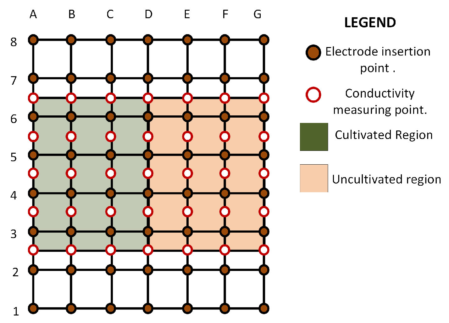
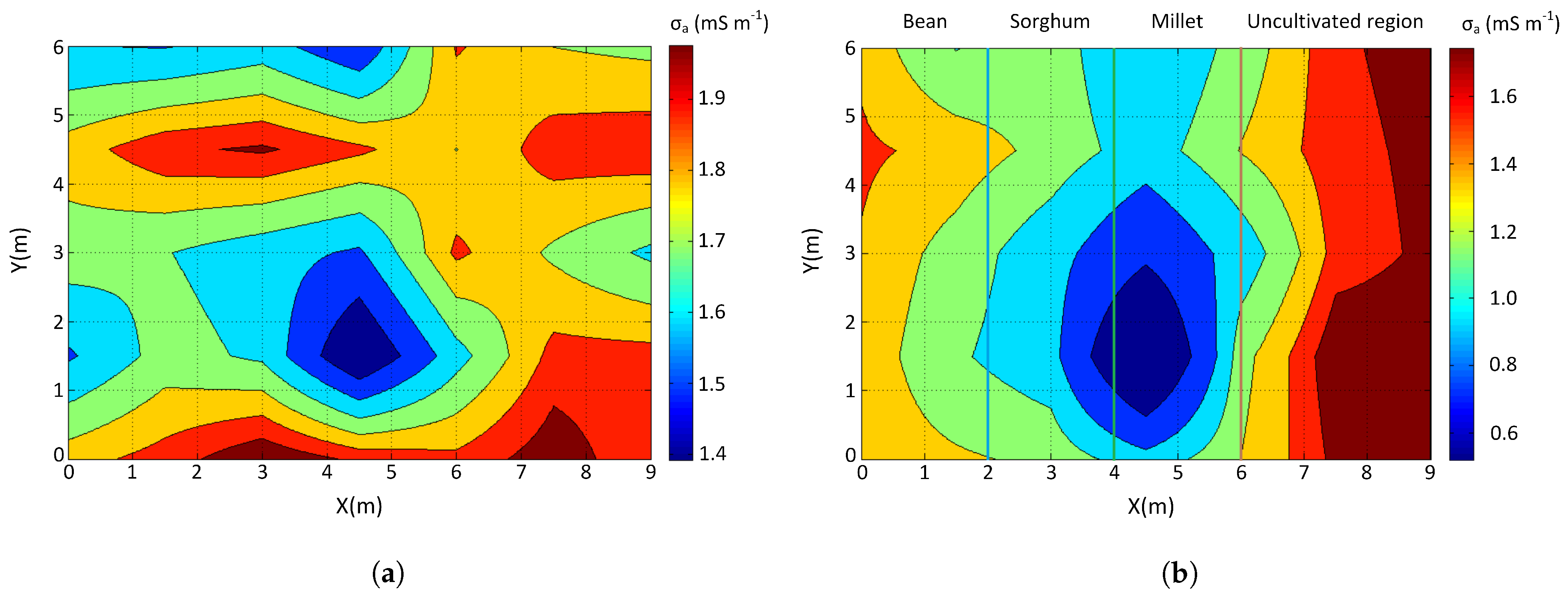
4.3. Root System Mapping in the Field

Field experiment was carried out on the Capivara farm, located in the city of Santo Antônio de Goias, Goias/Brazil, 16 30 05.9 S and 49 16 56 . 3 W. The region defined for the study has 9 m × 6 m and the lateral profiling method was used with a = 1.5 m spacing and P = 0.20 m depth. From R m measured values and (3), σ a data were obtained for R S mapping.
For the species cultivation chosen for the experiment, there was manual sowing of beans (Phaseolus vulgaris L.), sorghum (Sorghum bicolor L. Moench), and millet (Pennisetum glaucum L.) seeds, with 0.5 m spacing between rows. The reasons for choosing different cultures were to verify the possibility of the adopted geoprospecting method to detect different root systems over time. There were four planting lines of 6m for each cultivated species, resulting in a cultivated area of 36 m 2 and a reference area of 18 m 2 . For comparison purposes, the reference area was not cultivated.
Figure 17a shows the σ a spatial distribution in the study area before sowing crops and Figure 17b presents the σ a spatial distribution in the study area 62 days after sowing. In Figure 17, the indicative legend of σ a is translated into hot and cold colors only. There is no relation of colors between Figure 17a,b. The relationship occurs only between each legend of each Figure 17a,b. The σ a reduction 62 days after sowing was due to the cultures being in the flowering stage, when they have maximum root development. Additionally, in the cultivated region the apparent electrical conductivity of the soil was lower than in the non-cultivated region, indicating R S influence on σ a values. It was found that the R S that most influenced σ a was millet crop, followed by the sorghum and then bean crop.
Figure 17a presents the σ a mapping before the crops sowing, where the electrical conductivity variation is 1.4 < σ a < 2.0 [m · Sm 1 ] (regions in cold and hot colors, respectively). As plants develop, σ a values decrease and uniform zones of σ a values appear, as shown in Figure 17b, relating σ a with R S . Thus, the region cultivated with beans has 1.2 < σ a < 1.3 [m · Sm 1 ], the region cultivated with sorghum 1.0 < σ a < 1.2 [m · Sm 1 ] and the region cultivated with millet 0.6 < σ a < 1.0 [m · Sm 1 ].

5. Discussion

The survey of apparent electrical conductivity of the soil σ a in cultivated and uncultivated regions shows that geoelectric prospecting methods can be used to monitor plant root growth, by comparing σ a before and after sowing. Previous researchers have shown that soil electrical conductivity values are associated with plant growth [11,12,13,27]. However, this study shows root growth monitored in different periods and in cultivated and non-cultivated areas, both in laboratory and field study. Information from the reference soil, without plant cultivation, allows verifying the plant root system influence on the measured values of electrical conductivity of the soil and consequently analyze the dynamic growth of plant root mass.
The results of this study showed the σ a capacity as an indirect and non-invasive method of analyzing soil moisture and the plants R S growth. The increase in soil moisture content causes an increase in electrical conductivity of the soil up to the moisture saturation point, around 35%. On the other hand, the plants R S growth causes a decrease in σ a values.
Researchers have found low values of σ a (or high values of ρ a ) associated with plants root system [11,12,32]. This behavior can be observed, for example, in the laboratory experiment of this study where the 0.12 m length of millet roots after 30 days of sowing is consistent with the σ a reduction. In addition, the field study presents lower σ a values in the cultivated region than in the non-cultivated region.
Other works demonstrate the relationship between soil moisture and electrical conductivity, without analyzing what happens in depth [2,30,33]. However, soil stratification in horizontal layers makes it possible to observe the phenomenon of water percolation and the plants R S growth. The σ a at P 2 and P 3 depths increases in the first few days due to water and fertilizer leached from P 1 , indicating percolation and possibly other phenomena. The σ a monitoring in depth serves to analyze the soil dynamics, observing the hydraulic properties involving R S .
This paper was limited to performing measurements of moisture content and electrical conductivity of the soil to correlate with root mass of plants, without data collection referring to soil temperature. Analyzes of temperature and moisture, both at the soil surface and in depth, can be incorporated in future research to correlate soil moisture content, soil temperature and σ a with the plant root system.

6. Conclusions

The survey of the apparent electrical conductivity of the soil σ a is an approach for analyzing the soil moisture content ω and plants R S growth from the sowing period to maturation of cultures. Through σ a it is possible to observe the seasonal dynamics of the soil in relation to moisture, the roots development over time and the relation σ a × root mass. Furthermore, it was found that the soil stratification in horizontal layers allows the soil analysis in depth, being possible to use σ a as an instrument for analyzing the water percolation phenomenon in the soil and the roots development with indication of the place of root mass concentration in the soil.
The obtained results demonstrate that geoelectric prospecting methods can detect and indirectly monitoring the development of plant roots and mapping some variables that contribute to the soil dynamics. The proposed methodology can be used as a non-invasive method of mapping the root system of plants as well as verification of the downward movement of water to support localized irrigation, subsoiling and inputs application.

Author Contributions

Conceptualization, A.M.S.F., J.R.S.S., G.M.F., L.D.S.M.; methodology, A.M.S.F., J.R.S.S., G.M.F., L.D.S.M., W.P.C.; software, A.M.S.F., J.R.S.S., G.M.F., L.D.S.M., W.P.C.; validation, A.M.S.F., J.R.S.S., G.M.F., L.D.S.M., W.P.C.; formal analysis, A.M.S.F., J.R.S.S., G.M.F., L.D.S.M., W.P.C., A.P.C.; investigation, A.M.S.F., J.R.S.S., G.M.F., L.D.S.M., W.P.C., A.P.C.; resources, W.P.C.; writing—original draft preparation, A.M.S.F., J.R.S.S., G.M.F., L.D.S.M., W.P.C.; writing—review and editing, A.M.S.F., W.P.C., A.P.C.; visualization, W.P.C.; supervision, W.P.C.; project administration, W.P.C. All authors have read and agreed to the published version of the manuscript.

Funding

This research received no external funding.

Institutional Review Board Statement

Not applicable.

Informed Consent Statement

Not applicable.

Data Availability Statement

Not applicable.

Acknowledgments

The authors would like to thank the National Council for Scientific and Technological Development (CNPq), the Foundation for Research Support of the State of Goias (FAPEG), and the Brazilian Federal Agency for Support and Evaluation of Graduate Education (CAPES) for scholarships. They also thank the Federal Institute of Goias (IFG), Federal Institute of Tocantins (IFTO), Federal University of Goias/Faculty of Agronomy (UFG), and Embrapa Rice and Beans (EMBRAPA Arroz e Feijão/Goias) for supporting research in the form of laboratories, data, and input donation.

Conflicts of Interest

The authors declare no conflict of interest.

Abbreviations

The following abbreviations are used in this manuscript:
σ a apparent electrical conductivity of the soil
R S root system
ω soil moisture content
TDRTime Domain Reflectometry
Csoil compaction
R m apparent electrical resistance
ρ a apparent electrical resistivity of the soil
aspacing between rods in Wenner array
isummation variable
h 1 thickness of the first soil layer
h 2 thickness of the second soil layer
h 3 thickness of the third soil layer
Prods depth in Wenner array
Kreflection coefficient of the expression of soil stratification in two layers
ρ 1 apparent resistivity of the first soil layer
ρ 2 apparent resistivity of the second soil layer
ρ 3 apparent resistivity of the third soil layer
ρ 4 apparent resistivity of the fourth soil layer
MSPmoisture saturation point
Nnumber of layers
PVCpolyvinyl chloride
HDPEhigh-density polyethylene
T m a x ¯ average temperature data of the highs
T m i n ¯ average temperature data of the lows
P t o t total precipitation

References

  1. Telford, W.M.; Geldart, L.P.; Sheriff, R.E. Applied Geophysics; Cambridge University Press: Cambridge, UK, 1990. [Google Scholar]
  2. Corwin, D.L.; Lesch, S.M. Apparent soil electrical conductivity measurements in agriculture. Comput. Electron. Agric. 2005, 46, 11–43. [Google Scholar] [CrossRef]
  3. Silva Filho, A.M.; Silva, C.L.B.; Oliveira, M.A.A.; Pires, T.G.; Alves, A.J.; Narciso, M.G.; Calixto, W.P. Geoelectric method applied in correlation between physical characteristics and electrical properties of the soil. Trans. Environ. Electr. Eng. 2017, 2, 36. [Google Scholar] [CrossRef]
  4. Moral, F.J.; Terrón, J.M.; Marques da Silva, J.R. Delineation of management zones using mobile measurements of soil apparent electrical conductivity and multivariate geostatistical techniques. Soil Tillage Res. 2005, 106, 335–343. [Google Scholar] [CrossRef]
  5. Johnson, C.K.; Doran, J.W.; Duke, H.R.; Wienhold, B.J.; Eskridge, K.M.; Shanahan, J.F. Field-scale electrical conductivity mapping for delineating soil condition. Soil Sci. Soc. Am. J. 2001, 65, 1829–1837. [Google Scholar] [CrossRef] [Green Version]
  6. Serrano, J.M.; Shahidian, S.; Da Silva, J.M. Spatial variability and temporal stability of apparent soil electrical conductivity in a Mediterranean pasture. Precis. Agric. 2017, 18, 245–263. [Google Scholar] [CrossRef]
  7. Sanches, G.M.; Magalhães, P.S.G.; Remacre, A.Z.; Franco, H.C.J. Potential of apparent soil electrical conductivity to describe the soil pH and improve lime application in a clayey soil. Soil Tillage Res. 2018, 175, 217–225. [Google Scholar] [CrossRef]
  8. Li, H.Y.; Shi, Z.; Webster, R.; Triantafilis, J. Mapping the three-dimensional variation of soil salinity in a rice-paddy soil. Geoderma 2005, 195–196, 31–41. [Google Scholar] [CrossRef]
  9. Corwin, D.L.; Lesch, S.M.; Shouse, P.J.; Soppe, R.; Ayars, J.E. Identifying Soil Properties that Influence Cotton Yield Using Soil Sampling Directed by Apparent Soil Electrical Conductivity. Agron. J. 2003, 95, 352–364. [Google Scholar] [CrossRef] [Green Version]
  10. Cillis, D.; Pezzuolo, A.; Marinello, F.; Sartori, L. Field-scale electrical resistivity profiling mapping for delineating soil condition in a nitrate vulnerable zone. Appl. Soil Ecol. 2018, 123, 780–786. [Google Scholar] [CrossRef]
  11. Cimpoiaşu, M.O.; Kuras, O.; Pridmore, T.; Mooney, S.J. Potential of geoelectrical methods to monitor root zone processes and structure: A review. Geoderma 2020, 365, 114232. [Google Scholar] [CrossRef]
  12. Amato, M.; Basso, B.; Celano, G.; Bitella, G.; Morelli, G.; Rossi, R. In situ detection of tree root distribution and biomass by multi-electrode resistivity imaging. Tree Physiol. 2008, 28, 1441–1448. [Google Scholar] [CrossRef]
  13. Zhao, P.-F.; Wang, Y.-Q.; Yan, S.-X.; Fan, L.-F.; Wang, Z.-Y.; Zhou, Q.; Yao, J.-P.; Cheng, Q.; Wang, Z.-Y.; Huang, L. Electrical imaging of plant root zone: A review. Comput. Electron. Agric. 2019, 167, 105058. [Google Scholar] [CrossRef]
  14. Paglis, C.M. Application of Electrical Resistivity Tomography for Detecting Root Biomass in Coffee Trees. Int. J. Geophys. 2013. [Google Scholar] [CrossRef]
  15. Loperte, A.; Satriani, A.; Lazzari, L.; Amato, M.; Celano, G.; Lapenna, V.; Morelli, G. 2D and 3D high resolution geoelectrical tomography for non-destructive determination of the spatial variability of plant root distribution: Laboratory experiments and field measurements. Geophys. Res. Abstr. 2006, 8, 674. [Google Scholar]
  16. Head, K.H. Manual of Soil Laboratory Testin. In Soil Classification and Compaction Tests; Whittles Publishing: Scotland, UK, 2006; Volume 1. [Google Scholar]
  17. Soane, B.D.; van Ouwerkerk, C. Soil Compaction in Crop Production; Elsevier: Amsterdam, The Netherlands, 2013. [Google Scholar]
  18. Naderi-Boldaji, M.; Sharifi, A.; Hemmat, A.; Alimardani, R.; Keller, T. Feasibility study on the potential of electrical conductivity sensor Veris® 3100 for field mapping of topsoil strength. Biosyst. Eng. 2014, 126, 1–11. [Google Scholar] [CrossRef]
  19. Roodposhti, H.R.; Hafizi, M.K.; Kermani, M.R.S.; Nik, M.R.G. Electrical resistivity method for water content and compaction evaluation, a laboratory test on construction material. J. Appl. Geophys. 2019, 168, 49–58. [Google Scholar] [CrossRef]
  20. Friedman, S.P. Soil properties influencing apparent electrical conductivity: A review. Comput. Electron. Agric. 2005, 46, 45–70. [Google Scholar] [CrossRef]
  21. Corwin, D.L.; Lesch, S.M. Application of Soil Electrical Conductivity to Precision Agriculture. Agron. J. 2003, 95, 455–471. [Google Scholar]
  22. Corwin, D.L.; Lesch, S.M.; Oster, J.D.; Kaffka, S.R. Monitoring management-induced spatio–temporal changes in soil quality through soil sampling directed by apparent electrical conductivity. Geoderma 2006, 131, 369–387. [Google Scholar] [CrossRef]
  23. Wenner, F.A. Method of Measuring Earth Resistivity; Bulletin of National Bureau of Standards: Washington, DC, USA, 1916; Volume 12. [Google Scholar]
  24. IEEE Std 142 Recommended Practice for Grounding of Industrial and Commercial Power Systems. Available online: https://hibp.ecse.rpi.edu/connor/education/Fields/IEEEStd142_2007.pdf (accessed on 16 October 2021).
  25. Pirson, S.J. Geologic Well Log Analysis; Gulf Publishing Co.: Houston, TX, USA, 1963. [Google Scholar]
  26. Sudduth, K.A.; Myers, D.B.; Kitchen, N.R.; Drummond, S.T. Modeling soil electrical conductivity–depth relationships with data from proximal and penetrating ECa sensors. Geoderma 2013, 199, 12–21. [Google Scholar] [CrossRef]
  27. Banton, O.; Seguin, M.K.; Cimon, M.A. Mapping Field-Scale Physical Properties of Soil with Electrical Resistivity. Soil Sci. Soc. Am. J. 1997, 61, 1010–1017. [Google Scholar] [CrossRef]
  28. Hagrey, A. Numerical and experimental mapping of small root zones using optimized surface and borehole resistivity tomography. Geophysics 2011, 76, G25–G35. [Google Scholar] [CrossRef]
  29. Bohm, W. Methods of Studying Root Systems; Springer: New York, NY, USA, 1979. [Google Scholar]
  30. Melo, L.B.B.; Silva, B.M.; Peixoto, D.S.; Chiarini, T.P.A.; Oliveira, G.C.; Curi, N. Effect of compaction on the relationship between electrical resistivity and soil water content in Oxisol. Soil Tillage Res. 2021, 208, 104876. [Google Scholar] [CrossRef]
  31. Meteoblue. 2021. Available online: https://www.meteoblue.com (accessed on 1 April 2021).
  32. Amato, M.; Bitella, G.; Rossi, R.; Gómez, J.A.; Lovelli, S.; Gomes, J.J.F. Multi-electrode 3D resistivity imaging of alfalfa root zone. Eur. J. Agron. 2009, 31, 213–222. [Google Scholar] [CrossRef]
  33. Nijland, W.; van der Meijde, M.; Addink, E.A.; de Jong, S.M. Detection of soil moisture and vegetation water abstraction in a Mediterranean natural area using electrical resistivity tomography. Catena 2009, 81, 209–216. [Google Scholar] [CrossRef]
Figure 1. Simplified constitution and main current pathways in the soil.
Energies 14 06951 g001
Figure 2. Lateral Profiling Method.
Energies 14 06951 g002
Figure 3. Flow of the proposed methodology: (a) relationship between ω × σ a and (b) relationship between R S ×   σ a .
Energies 14 06951 g003
Figure 4. Illustration of the container used to compare σ a × ω .
Energies 14 06951 g004
Figure 5. Directions for applying the Wenner array.
Energies 14 06951 g005
Figure 6. Illustration of the container used to compare σ a × R S in laboratory: (a) front view and (b) upper view.
Energies 14 06951 g006
Figure 7. Area delimitation to apply the proposed method to compare σ a × R S in field.
Energies 14 06951 g007
Figure 8. Instruments used to map R m × ω .
Energies 14 06951 g008
Figure 9. Results of: (a) ω × R m and (b) ω × σ a .
Energies 14 06951 g009
Figure 10. Directions and spacing used for the Wenner arrangement.
Energies 14 06951 g010
Figure 11. The σ a × a curve in the same soil for dry and rainy periods.
Energies 14 06951 g011
Figure 12. Soil stratification using the Pirson method: (a) layers thickness and (b) layers resistivity.
Energies 14 06951 g012
Figure 13. Container arrangement for collecting data of σ a × days of laboratory cultivation.
Energies 14 06951 g013
Figure 14. Average variation of σ a × days of cultivation for data collected in the laboratory.
Energies 14 06951 g014
Figure 15. Root growth mapping: (a) start of experiment on the seventh day and (b) end of experiment to the seventy-fourth day.
Energies 14 06951 g015
Figure 16. Relationship between σ a × root mass.
Energies 14 06951 g016
Figure 17. Spatial distribution of σ a in the delimited area of 54 m 2 : (a) before sowing crops and (b) 62 days after sowing the crops.
Energies 14 06951 g017
Table 1. Temperature and precipitation data for dry and rainy periods.
T max ¯ [ C ] T min ¯ [ C ] P tot [mm]
Dryseason 1312184
Dryseason 2271889
Rainyseason 12619225
Rainyseason 22619171
Table 2. Thickness and resistivity values per layer for dry and rainy periods.
Thickness [m]Resistivity [ Ω · m]
h 1 h 2 h 3 h 4 ρ 1 ρ 2 ρ 3 ρ 4
Dryseason 10.406.656.435175.9318,009.901806.9610,684.20
Rainyseason 10.376.519.825175.9318,173.001895.757120.07
Publisher’s Note: MDPI stays neutral with regard to jurisdictional claims in published maps and institutional affiliations.

