
Real Driving Emissions in Extended Driving Conditions

1
AFHB, University of Applied Sciences TI, 2500 Biel-Bienne, Switzerland
2
CJ Consulting, 2562 Port, Switzerland
3
Federal Office for the Environment (FOEN), Air Pollution Control and Chemicals Division, 3003 Bern, Switzerland
*
Author to whom correspondence should be addressed.
Energies 2021, 14(21), 7310; https://doi.org/10.3390/en14217310
Submission received: 17 August 2021
/
Revised: 10 October 2021
/
Accepted: 16 October 2021
/
Published: 4 November 2021
(This article belongs to the Special Issue Recent Advances in Internal Combustion Engines)
Abstract
:The real driving emission (RDE) testing for certification of vehicles is performed in conditions that are well defined in legislation. For emissions inventories and for research, the influences of some extended driving conditions on emissions are an interesting issue. In the present work, some examples of RDE results from two common passenger cars with gasoline and diesel propulsion are given. The varying driving conditions were “winter/summer”, “mild/aggressive”, and “higher altitude/slop”. The driving conditions: “winter”, “aggressive”, and “higher slope/altitude” generally require more energy, cause higher fuel consumption, and therefore, higher CO2-emissions. The condition of “winter driving”, especially in the urban type of operation, may cause some longer phases with not enough warmed-up exhaust aftertreatment and consequently some increased gaseous emissions. The DPF eliminates the nanoparticles (PN) independently on the driving conditions. Nevertheless, the DPF regeneration has an influence on the CO2-normality of the trip. The CO2-normality primary tolerance range can also be exceeded with aggressive driving. The elaborated results confirm the usefulness of the existing legal limits for the driving conditions of RDE homologation tests.
1. Introduction
The testing and evaluating of real driving emissions (RDE) as a part of the certification of new types of passenger cars was introduced into EU-legislation in September 2017. Different details concerning the development and refining of testing procedure, testing equipment, evaluation, and others were introduced in so-called RDE packages. The fourth RDE package applies for certification since January 2019. The most important innovations and amendments of RDE4 vs. RDE3 concern [1]:
- Specifications and calibration of PEMS components and signals.
- Verification of overall trip dynamics with MAW (moving average windows) and with RPA (relative positive acceleration).
- Determination of the cumulative positive elevation gain of a PEMS trip.
- Calculation of final RDE emissions.
- Data exchange and reporting requirements.
- Provisions for in-service-conformity (ISC).
Great importance was attached to in-service-conformity (ISC) testing and reporting (article 9). The responsibility for ISC is shifted to granting type approval authorities (GTAA’s), external specialized laboratories, or technical services. Extensive useful information about the application of the RDE packages can be found in specific literature and on the internet [2,3,4,5,6,7]. Collection of RDE-data offers several synergies. The increased amount of RDE-data can be used for different objectives, such as: further development of emission inventories, compliance with “In-Service Conformity” (ISC, EU regulation 2018/1832), and market surveillance activities (EU regulation 2018/858). Emission factors and emission inventories are an important source of data for compiling and modelling the emissions of traffic in different situations. There is in the EU, continuous work and development of emission data inventories [8,9,10,11,12].
Extensive activities of testing RDE by means of PEMS (portable emissions measuring systems) have been performed in recent years, aiming not only at emissions, but also the improvements of instrumentation, of testing procedures, and of evaluation [13,14,15,16,17,18,19,20,21,22,23]. The test for certification purposes have to be performed in driving conditions, like ambient temperature, altitude, or driving dynamics, which are defined in the regulations according to the most commonly appearing ranges. For emissions inventories, some other (extended) driving conditions are of interest. Therefore, several studies have tried to determine the influence of boundary conditions such as ambient temperature (winter/summer). Driving style (aggressive/mild) as well as the influence of slope and geodesic height. These different factors were addressed by the authors in [23,24,25,26,27,28,29,30]. The entirety of these factors will now be presented in the present paper to give some examples of influences of the extended driving conditions on the emissions and on the (certification) validity of the trip for two typical passenger cars (gasoline and diesel). The tests were performed by the Laboratory for Exhaust Emissions Control (AFHB) of the Berne University of Applied Sciences (BFH-TI), Biel-Bienne, Switzerland.
2. Testing Material, Means, and Methods
2.1. Test Vehicles and Uesd Gas PEMS and PN PEMS
The tests with extended driving conditions were performed on two vehicles V1 (Gasoline Euro 5) and V2 (Diesel Euro 6). The most important data of these vehicles are listed in Table 1.
All vehicles were operated with the Swiss market fuels and with lubricating oils, which were present in each vehicle.
2.2. Gas PEMS and PN PEMS
For measurements of gaseous components, the system Horiba PEMS OBS-ONE was used. The most important data of this GasPEMS system are given in the Table 2. As PN PEMS for Real Driving Emissions two systems were used:
- Horiba OBS-ONE PN measurement system (OBS-PN). This analyzer works on the condensation particles counter (CPC) principle, has an integrated sample conditioning system (double dilution and catalytic stripper ViPR, 350 °C), and it indicates the summary PN concentrations in the size range 23 to approximately 1000 nm.
- NanoMet3 from TESTO (NM3). This analyzer works on diffusion charging (DC) principle, has an integrated sample conditioning system, and it indicates the solid particle number concentration and geometric mean diameter in the size range 10–700 nm.
For the exhaust gas sampling and conditioning of the NM3 a ViPR system (ViPR…volatile particle remover) from Matter Aerosol was used. This system contains:
- Primary dilution—MD19 tunable rotating disk diluter (Matter Eng. MD19-2E).
- Secondary dilution—dilution of the primary diluted and thermally conditioned sample gas on the outlet of evaporative tube.
- Thermoconditioner (TC)—sample heating at 300 °C.
Both PN PEMS present several advantages like compactness, robustness, fast on-line response and both are recognized for legal testing purposes.
2.3. Test Procedures
The RDE tests were performed on the road in real driving conditions. For all tests, except of higher slope/altitude the standard and legally valid AFHB-route was used. (More information about the routes with higher slope/altitude is given in the “results”). All tests were started with cold engine. The ambient temperatures were in the range of 20 °C, except of the winter attempts with tamb in the range of 5 °C.
The evaluation of data was performed according to the legal requirements with EMROAD program, package RDE 4.
3. Results
3.1. Winter/Summer Conditions
Figure 1 shows an example of cumulated RDE results obtained with the gasoline vehicle (V1) in winter driving conditions. There were, respectively, three repetitions performed on the official RDE-circuit. Some emissions differences between the repeated tests are caused by different traffic situations and driving behavior. Especially stronger accelerations, mainly in the urban part, can produce higher emissions increments.
Figure 2 summarizes and compares the results of the gasoline vehicle (V1). Considering the averages of three repetitions, it can be followed that in winter conditions, there are higher values of CO2 and CO in the total trip. For NOX and PN, there are no significant differences. There are unfortunately no measured values for THC. However, according to the general experience, the tendencies of HC are in line with the tendencies of CO. The winter in the season 2019/2020 was quite mild with the ambient day temperatures around 5 °C. Figure 3 shows an example of cumulated RDE results obtained with the diesel vehicle (V2) in summer driving conditions.
In both test series (summer and winter), one of the repetitions was with DPF regeneration, which was ordinarily triggered by the electronic control system of the vehicle. The plots “with regeneration” are here presented, together with one of the trials “without regeneration”. The regeneration increases clearly the represented emissions. Figure 4 summarizes and compares the results of the diesel vehicle (V2). Considering the averages of the three repetitions, it can be remarked that the winter-operation increases slightly the CO2- and NOx-values. The levels of CO, THC, and PN stay unchanged. The regeneration increases clearly (both in summer and in winter tests) CO2-, NOx-, and PN-values. There are no visible effects on CO and very slight increase of THC, which, being at a very low absolute level, may be considered as insignificant. It can be stated that in these testing conditions of a quite mild winter period, the effect of regeneration on several emission components is stronger than the effect of the lower ambient temperature of the winter driving conditions. The fact of increased emissions (especially PN and NOx) during the DPF regeneration is well known and the type approval legislation considers it adequately by averaging the regeneration cycles with the non-regeneration ones.
3.2. Mild/Aggressive Driving
For each vehicle and each variant of driving style, three tests were performed. Figure 5 represents the validity check of driving dynamics for both vehicles. In the top part of the figure, the definition and the legal limit line of the relative positive acceleration (RPA) are given. All results are in the domain “pass”, i.e., the check, if the trip dynamics is not too weak, is fulfilled. In the bottom part of the figure, the legal limit line of [95% of v. apos] is represented. The domain “fail” means that there are a too hard driving behavior and excessive dynamics of the trip. This is the case for aggressive driving style with the diesel vehicle (this type of vehicles is constructed and well-known for the high torque characteristics at lower engine speeds). It can be concluded that:
- The mild and dynamic driving styles have clearly different parameters of the RPA and (v.a pos); both parameters are higher for aggressive driving.
- During road driving, the parameters of the RPA and (v.apos) are for each variant of vehicle and driving style quite repetitive.
- With the diesel vehicle, an excessive driving dynamic, beyond the legal acceptance, was realized.
Figure 6 shows the CO2-normality check for both vehicles. The normality check that is the comparison of CO2 emissions during the RDE-measurement using MAW with the reference CO2-emissions obtained on the chassis dyno during the WLTC. For the gasoline vehicle (in the top part of the figure), there are clearly higher CO2-values at dynamic driving, but the trips and their dynamic conditions are entirely normal since the characteristic curves are not exceeding the primary tolerance band of +45(40)/−25% (of the average WLTC-CO2-values). The CO2-normality check for diesel vehicle is represented in the bottom part of the figure. In the highest speed range and with “mild” operation, the characteristic line exceeds the primary tolerance domain +45(40)/−25%. In one of the trials with “mild” operation, DPF regeneration happened. This had consequences on CO2-values and caused them to exceed the primary tolerance band as well at the lowest speed range. It can be concluded that:
- The driving style has an influence on the CO2-normality.
- The normality check is also passed with the dynamic driving style.
- The DPF regeneration (diesel) has an influence on the CO2-normality, which may cause the check to fail.
Figure 7 represents the influences of driving style on the cumulated emissions of CO, NOx, CO2, and PN of the gasoline car for, respectively, three “mild” and “dynamic” tests. The following relationships can be remarked:
- The driving style has a very strong influence on CO-emissions and the results from the three tests are quite repetitive (except for highway).
- The driving style also influences strongly the NOx-emissions during cold start and city part; in case of aggressive driving in the urban part, the NOx-values scatter vary much which also explains the large differences of cumulated NOx with the “dynamic” driving.
- The “dynamic” driving requires more energy, causes higher fuel consumption, and, therefore, higher CO2-emissions.
- There is no visible effect of driving style on the PN-emissions, the absolute values in (#/km) for this GDI-vehicle, without GPF are quite high, above the legal limit of 6 × 10¹¹ (#/km).
Figure 8 shows the influences of the driving style on the cumulated emissions of CO, NOx, CO2, and PN of the diesel car. The logic of the representation is the same as in Figure 7. The following relationships of emissions can be remarked for this vehicle V2:
- The CO-emissions are very low and they are independent of the driving style.
- All other emissions of NOx, CO2, and PN are clearly increased by the dynamic driving style.
A rough comparison of emissions of both test vehicles (V1 gasoline Euro 5 and V2 Diesel Euro 6) shows the same typical proportions: higher CO, higher CO2, and higher PN (w/o GPF) values for gasoline V1; higher NOx and lower PN (with DPF) for diesel V2. Figure 9 summarizes the variations of the emissions in (%) between mild and dynamic driving style. The higher variations of NOx and CO2 in the urban part can be generalized as an effect of higher dynamics in city driving. The very high variations of CO of the gasoline car (especially in the rural- and highway parts) must be considered as specific for this vehicle. They certainly could be changed by the measures lowering these emissions (CO) of this vehicle. The PN-emissions of the diesel vehicle are at a very low level (due to DPF) and the driving style has a stronger percentual influence than with the gasoline vehicle (GDI w/o GPF).
3.3. Higher Slope/Altitude
In this working package, the results obtained on a normal legally valid circle were compared with two other “high altitude” circles. The normal route is called in further diagrams as “cir1”. The other two routes are: RDE route with higher altitude variations, “cir2” (Pierre-Pertuis, Tavannes), and RDE route at high altitude, “cir3” (plateau de Diesse). Examples of the speed profiles and the traces of altitude of these test circuits are illustrated in Figure 10.
These routes (cir2 and cir3) do not legally conform and they are defined and used only for the research in the present working package. Some legal requirements concerning the altitude of the test route are given in the Regulation EU 2017/1151, annex IIIa, appendix 7b. These are:
- Moderate altitude below 700 m above sea level.
- Extended altitude conditions 700–1300 m above sea level.
- Start and end points of the trip shall not differ in their altitudes more than 100 m.
- The cumulative positive gain over the entire trip shall be less than 1200 m/100 km.
For the test circles used in the present work, it must be remarked that, principally, the rural part was decisive for the influences of slope and altitude. The city and highway parts were always the same and more or less flat. The variations of altitude have impact on the final results by increasing or decreasing the work amount provided by the vehicle. Figure 11 illustrates the validity check of the three used routes/trips. The trips “cir2” and “cir3” with higher altitude variations do not fulfill entirely the CO2-normality, exceeding the primary tolerance band of +45(40)/−25% in the middle speed range.
The checks of the share of normal windows (r) and of the total cumulative positive elevation gain (in the bottom part of the Figure 11) also show the non-conformity of the trips cir2 and cir3:
- Route cir2 could be accepted for elevation check, but the increase of the CO2 emissions due to the performed altitude variation leads to a failing CO2 result (not similar to the WLTC CO2 emissions).
- Route cir3 shows that both CO2 emissions and higher altitude variation are beyond the accepted limits.
The altitude data are measured by GPS and verified with topographic map. If the differences between the GPS data and the map is greater than 40 m, the GPS data are corrected. The Figure 12 compares the cumulated emissions CO, NOx, CO2, PN of the gasoline car in the three circuits with different slope and altitude. The results concern entire trips, which all were started with cold engine. The higher slope and/or altitude generally increase CO & NOx, have a slight influence on CO2, and a negligible influence on PN. (For PN see the very much extended scale of the ordinate).
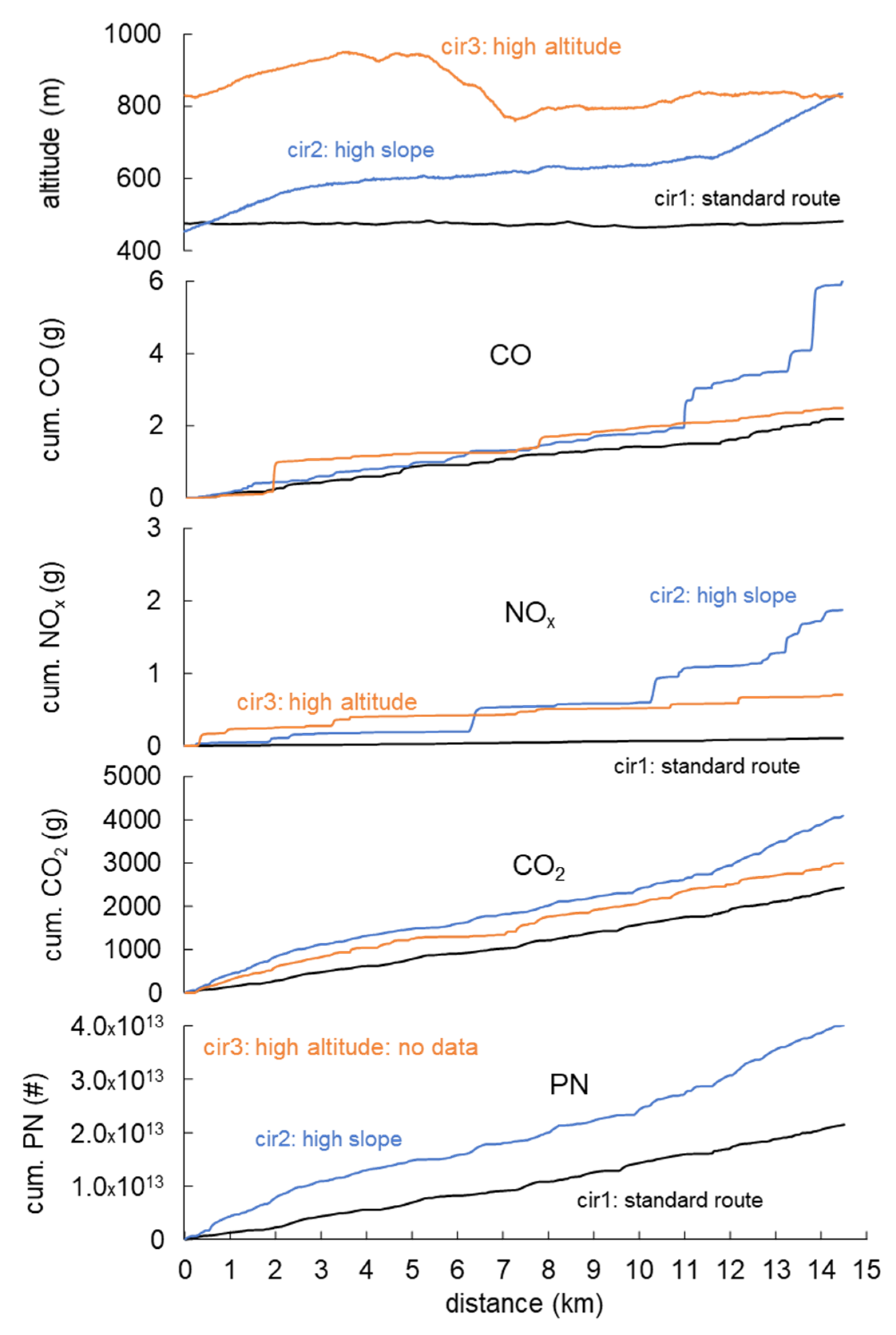
In order to better discriminate the influences of the altitude and the slope on the emissions, selected parts of trips were taken into consideration. Figure 13 represents the selected segments, all of them with the same driving distance (14.5 km) and with similar average speed (approximately 51 km/h). In this way, the segment chosen from the cir2 represents predominantly the high slope and the segment chosen from the cir3 represents mainly the high altitude. The results of evaluations with this part selection are given in Figure 14. The representation is analogous as in the Figure 12. The statement about increasing the measured emissions by higher slope and/or altitude can be extended to all components. The sharp increases of CO and NOx in the diagram for cir2 and cir3 can be attributed to the dynamic driving events combined with higher power demand for the slope. Higher slope (cir2) in this comparison needs more energy and emits more CO2 than the high-altitude profile (cir3).
4. Conclusions
The different driving conditions in real drive scenarios are ambient temperature (winter/summer), driving style (aggressive/mild), as well as the influence of slope and the altitude. These factors have been evaluated after performing tests in these different extended (non-typical) driving conditions. The expected influences on the individual emissions types could be shown according to the generally valid correlations on how the emission increase or decrease. In the following conclusions can be drawn:
Winter/summer
- For the gasoline vehicle, there are in winter conditions higher values of CO2 and CO in the total trip. For NOx and PN, there are no significant differences.
- For the diesel vehicle, the winter-operation increases slightly the CO2- and NOx-values. The levels of CO and PN stay unchanged.
- The DPF regeneration increases clearly (both in summer and in winter tests) CO2-, NOx-, and PN-values.
Mild/aggressive driving
- The mild and dynamic driving styles have clearly different parameters of the RPA and (v.apos); both parameters are higher for aggressive driving.
- During road driving, the parameters of the RPA and (v.apos) are for each variant of vehicle and driving style quite repetitive.
- With the diesel vehicle, an excessive driving dynamic, beyond the legal acceptance, was realized.
- The driving style has an influence on the CO2-normality.
- The DPF regeneration (Diesel) has an influence on the CO2-normality, which may cause the check to fail.
- The driving style has reproducible effects on the emissions.
- The aggressive driving generally increases the emissions, except PN for gasoline car (w/o GPF) and CO for diesel car (DOC + DPF).
- The “dynamic” driving requires more energy, causes higher fuel consumption, and, therefore, higher CO2-emissions.
- The PN-emissions of the gasoline vehicle (GDI w/o GPF) are above, the PN-emissions of the diesel vehicle (with DPF) are below the limit value of 6 × 10¹¹ (#/km).
- There is a higher NOx-emissions level of the diesel car.
Slope/altitude
- The emissions of CO, NOx, CO2, and PN are generally increased by higher slope/altitude.
- The sharp increases of CO and NOx in the diagrams for cir2 and cir3 can be attributed to the dynamic driving events combined with higher power demand for the slope.
- Higher slope requires more energy and causes higher CO2.
- The influence on PN is small.
Author Contributions
Conceptualization, D.E. and J.C.; methodology, D.E. and J.C.; software, Y.Z.; validation, D.E. and Y.Z.; formal analysis, D.E. and Y.Z.; investigation, Y.Z.; resources, Y.Z.; data curation, Y.Z.; writing—original draft preparation, D.E.; writing—review and editing, D.E., J.C. and P.B.; visualization, Y.Z.; supervision, D.E.; project administration, D.E. All authors have read and agreed to the published version of the manuscript.
Funding
This research was funded by the Swiss Federal Offices for Environment (FOEN).
Acknowledgments
The authors express gratitude to the Swiss Federal Offices for Environment (FOEN) for the financial support of these activities.
Conflicts of Interest
The funders had no role in the design of the study; in the collection, analyses, or interpretation of data; in the writing of the manuscript, or in the decision to publish the results.
Abbreviations
| AFHB | Abgasprüfstelle FH Biel, CH |
| BFH-TI | Bern University of Applied Sciences, Engineering and Information Technology |
| CF | Conformity Factor |
| cir | test circuit |
| CLD | Chemoluminescence Detector |
| CPC | condensation particles counter |
| DC | diffusion charging |
| DI | Direct Injection |
| DOC | Diesel Oxidation Catalyst |
| DPF | Diesel Particle Filter |
| ECU | Engine Control Unit |
| EFM | Exhaust Flow Meter |
| EGR | Exhaust gases recirculation |
| EU | European Union |
| EMROAD | Data processing reference software |
| FID | Flame Ionization Detector |
| FOEN | Federal Office of Environment, CH |
| GDI | gasoline direct injection |
| GPF | Gasoline particulate filter |
| GPS | Global Positioning System |
| GTAA | Granting Type Approval Authority |
| ICE | Internal Combustion Engine |
| ISC | in-service-conformity |
| LD | Light Duty (personal car) |
| LDV | Light Duty Vehicle |
| MAW | Moving Average Window |
| MD | rotating disc minidiluter |
| NDIR | Non-Dispersive Infrared |
| NM3 | NanoMet3 |
| OBD | On Board Diagnosis |
| OBS | Horiba on board system |
| PC | passenger car |
| PEMS | Portable Emissions measurement system |
| PN | Particle Number |
| r | share of normal windows (MAW) |
| RDE | Real Driving Emission |
| ResRDE | research of RDE |
| RPA | Relative Positive Acceleration |
| SCR | Selective Catalytic Reduction |
| TC | thermo-conditioner |
| TWC | Three-way catalyst |
| V | vehicle |
| ViPR | volatile particle remover |
| WLTC | World Light-Duty Transient Cycle |
| WP | working package |
References
- Commission Regulation (EU) 2017/1151 of 1 June 2017, Supplementing Regulation (EC) No 715/2007. Available online: http://data.europa.eu/eli/reg/2017/1151/2020-01-25 (accessed on 15 October 2021).
- Schöggl, M. EU-Update Draft RDE Package 4. AVL Emission TechDay 2018, 6 April 2018. Available online: https://www.avl.com/documents/1982862/8084402/10_RDE+-+Real+Driving+Emissions+-+was+steckt+wirklich+dahinter.pdf (accessed on 15 October 2021).
- Changes to the Motor Vehicle Type-Approval System in the European Union. Policy Update ICCT-May 2018. Available online: www.theicct.org (accessed on 15 October 2021).
- PEMS Guidance Document. Available online: https://publications.jrc.ec.europa.eu/repository/handle/JRC95958 (accessed on 15 October 2021).
- 2017 PEMS Uncertainty Assessment. Available online: http://publications.jrc.ec.europa.eu/repository/bitstream/JRC109841/kjna29138enn.pdf (accessed on 15 October 2021).
- Questions and Answers on RDE. Available online: https://circabc.europa.eu/sd/a/7e0496c2-67fb-4468-9755-dfd93917d38a/Q%26A%20RDE%20vs2.pdf (accessed on 15 October 2021).
- EMROAD Tool and Exchange Sample Files. Available online: https://circabc.europa.eu/ui/group/f4243c55-615c-4b70-a4c8-1254b5eebf61/library/79a4a9b6-4003-4e02-956d-048dcef1a169 (accessed on 15 October 2021).
- European Environment Agency. EMEP/EEA Air Pollutant Emission Inventory Guidebook 2016; EEA Report. No 21/2016; European Environment Agency: Copenhagen, Denmark, 2016; Available online: https://www.eea.europa.eu//publications/emep-eea-guidebook-2016 (accessed on 29 March 2019).
- Valverde, V.; Mora, B.A.; Clairotte, M.; Pavlovic, J.; Suarez-Bertoa, R.; Giechaskiel, B.; Astorga-LLorens, C.; Fontaras, G. Emission Factors Derived from 13 Euro 6b Light-Duty Vehicles Based on Laboratory and On-Road Measurements. Atmosphere 2019, 10, 243. [Google Scholar] [CrossRef] [Green Version]
- Franco, V.; Kousoulidou, M.; Muntean, M.; Ntziachristos, L.; Hausberger, S.; Dilara, P. Road vehicle emission factors development: A review. Atmos. Environ. 2013, 70, 84–97. [Google Scholar] [CrossRef]
- Ntziachristos, L.; Gkatzoflias, D.; Kouridis, C.; Samaras, Z. COPERT: A European road transport emission inventory model. In Information Technologies in Environmental Engineering; Athanasiadis, P.A., Mitkas, A.E., Rizzoli, J., Gómez, M., Eds.; Springer: New York, NY, USA, 2009; pp. 491–504. [Google Scholar]
- Giechaskiel, B.; Gioria, R.; Carriero, M.; Lähde, T.; Forloni, F.; Perujo, A.; Martini, G.; Bissi, L.M.; Terenghi, R. Emission Factors of a Euro VI Heavy-Duty Diesel Refuse Collection Vehicle. Sustainability 2019, 11, 1067. [Google Scholar] [CrossRef] [Green Version]
- Andersson, J.; May, J.; Favre, C.; Bosteels, D.; de Vries, S.; Heaney, M.; Keenan, M.; Mansell, J. On-Road and Chassis Dynamometer Evaluations of Emissions from Two Euro 6 Diesel Vehicles. SAE Int. J. Fuels Lubr. 2014, 7, 919–934, SAE Technical Paper 2014-01-2826. [Google Scholar] [CrossRef] [Green Version]
- Bielaczyc, P.; Woodburn, J.; Szczotka, A. Exhaust Emissions of Gaseous and Solid Pollutants Measured over the NEDC, FTP-75 and WLTC Chassis Dynamometer Driving Cycles. 2019. Available online: https://www.sae.org/publications/technical-papers/content/2016-01-1008/ (accessed on 18 October 2021).
- May, J.; Bosteels, D.; Favre, C. An Assessment of Emissions from Light-Duty Vehicles using PEMS and Chassis Dynamometer Testing. SAE Int. J. Engines 2014, 7, 1326–1335. [Google Scholar] [CrossRef] [Green Version]
- Clairotte, M.; Valverde, V.; Bonnel, P.; Giechaskiel, B.; Carriero, M.; Otura, M.; Fontaras, G.; Pavlovic, J.; Martini, G.; Krasenbrink, A.; et al. Joint Research Centre, Light-Duty Vehicles Emissions Testing; Publications Office of the European Union: Luxembourg, 2018. [Google Scholar]
- Czerwinski, J.; Zimmerli, Y.; Comte, P.; Bütler, T. Experiences and Results with different PEMS. In Proceedings of the TAP Paper, International Transport and Air Pollution Conference, Lyon, France, 24–26 May 2016. [Google Scholar]
- Czerwinski, J.; Zimmerli, Y.; Comte, P.; Cachon, L.; Riccobono, F. Potentials of the portable emission measuring systems (PN PEMS) to control real driving emissions (RDE). In Proceedings of the 38 International Vienna Motor Symposium, Vienna, Austria, 27–28 April 2017; Volume 2. VDI Fortschritt-Bericht, Reihe 12, Nr. 802. [Google Scholar]
- Czerwinski, J.; Comte, P.; Zimmerli, Y.; Cachon, L.; Remmele, E.; Huber, G. Research of Emissions with Gas PEMS and PN PEMS. In Proceedings of the TAP Paper, International Transport and Air Pollution Conference, EMPA, Zürich, Switzerland, 15–16 November 2017. [Google Scholar]
- Giechaskiel, B.; Roccobono, F.; Bonnel, P. Feasibility Study on the Extension of the Real Driving Emissions (RDE) Procedure to Particle Number (PN); European Commission, Joint Research Centre: Ispra, Italy, 2015; ISBN 978-92-79-51003-8. ISSN 1831-9424. [Google Scholar] [CrossRef]
- Suarez-Bertoa, R.; Valverde, V.; Clairotte, M.; Pavlovic, J.; Giechaskiel, B.; Franco, V.; Kregar, Z.; Astorga, C. On-road emissions of passenger cars beyond the boundary conditions of the real-driving emissions test. Environ. Res. 2019, 176, 108572. [Google Scholar] [CrossRef] [PubMed]
- O’Driscoll, R.; Stettler, M.E.J.; Molden, N.; Oxley, T.; ApSimon, H.M. Real world CO2 and NOX emissions from 149 Euro 5 and 6 diesel, gasoline and hybrid passenger cars. Sci. Total Environ. 2018, 621, 282–290. [Google Scholar] [CrossRef] [PubMed]
- Luján, J.M.; Bermúdez, V.; Dolz, V.; Monsalve-Serrano, J. An assessment of the real-world driving gaseous emissions from a Euro 6 light-duty diesel vehicle using a portable emissions measurement system (PEMS). Atmos. Environ. 2018, 174, 112–121. [Google Scholar] [CrossRef]
- Bodisco, T.; Zare, A. Practicalities and Driving Dynamics of a Real Driving Emissions (RDE) Euro 6 Regulation Homologation Test. Energies 2019, 12, 2306. [Google Scholar] [CrossRef] [Green Version]
- Deppenkemper, K.; Ehrly lng, M.; Schoenen, M.; Koetter, M. Super Ultra-Low NOX Emissions under Extended RDE Conditions—Evaluation of Light-Off Strategies of Advanced Diesel Exhaust Aftertreatment Systems; SAE Technical Paper 2019-01-0742; SAE International: Detroit, MI, USA, 2019. [Google Scholar] [CrossRef]
- Bielaczyc, P.; Szczotka, A.; Woodburn, J. The effect of a low ambient temperature on the cold-start emissions and fuel consumption of passenger cars. J. Automob. Eng. 2011, 225, 1253–1264. [Google Scholar] [CrossRef]
- Dardiotis, C.; Martini, G.; Marotta, A.; Manfredi, U. Low-temperature cold-start gaseous emissions of late technology passenger cars. Appl. Energy 2013, 111, 468–478. [Google Scholar] [CrossRef]
- Suares-Bertoa, R.; Astorga, C. Impact of cold temperature on Euro 6 passenger car emissions. Environ. Pollut. 2018, 234, 318–329. [Google Scholar] [CrossRef] [PubMed]
- Merkisz, J.; Pielecha, J.; Jasiński, R. Remarks about Real Driving Emissions tests for passenger cars. Arch. Transp. 2016, 39, 51–63. [Google Scholar] [CrossRef]
- Williams, R.; Andersson, J.; Hamje, H.; Ziman, P.; Kar, K.; Fittavolini, C.; Pellegrini, L.; Gunther, G.; Oliva, F.; Van de Heijning, P. Impact of Demanding Low Temperature Urban Operation on the Real Driving Emissions Performance of Three European Diesel Passenger Cars; SAE Technical Paper 2018-01-1819; SAE International: Detroit, MI, USA, 2018. [Google Scholar] [CrossRef]
Figure 1.
Example of cumulated emissions in winter, official RDE route, vehicle 1, gasoline.
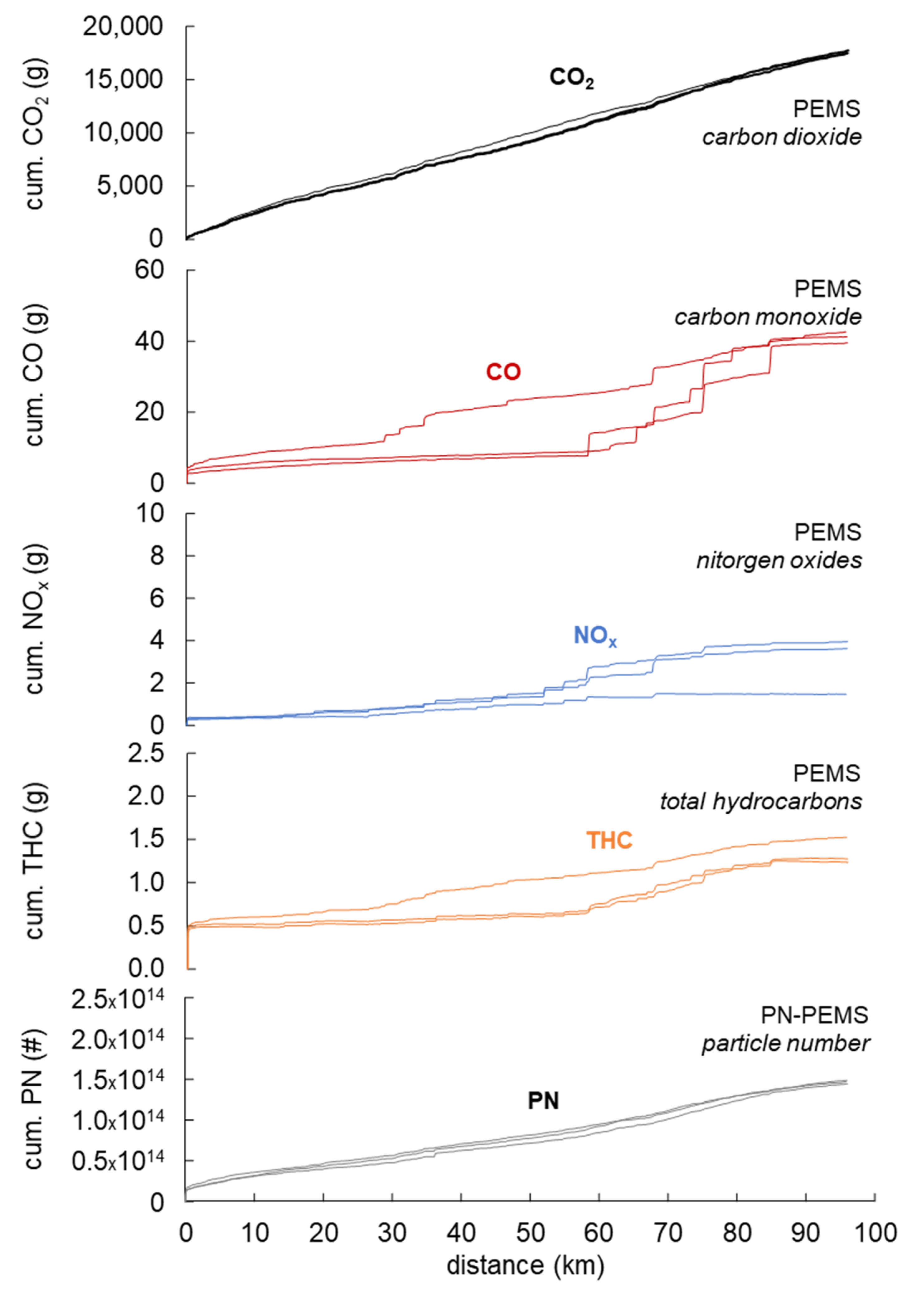
Figure 2.
Comparison of real driving emissions in summer and winter conditions, official RDE route, integral average values, vehicle 1, gasoline.
Figure 2.
Comparison of real driving emissions in summer and winter conditions, official RDE route, integral average values, vehicle 1, gasoline.
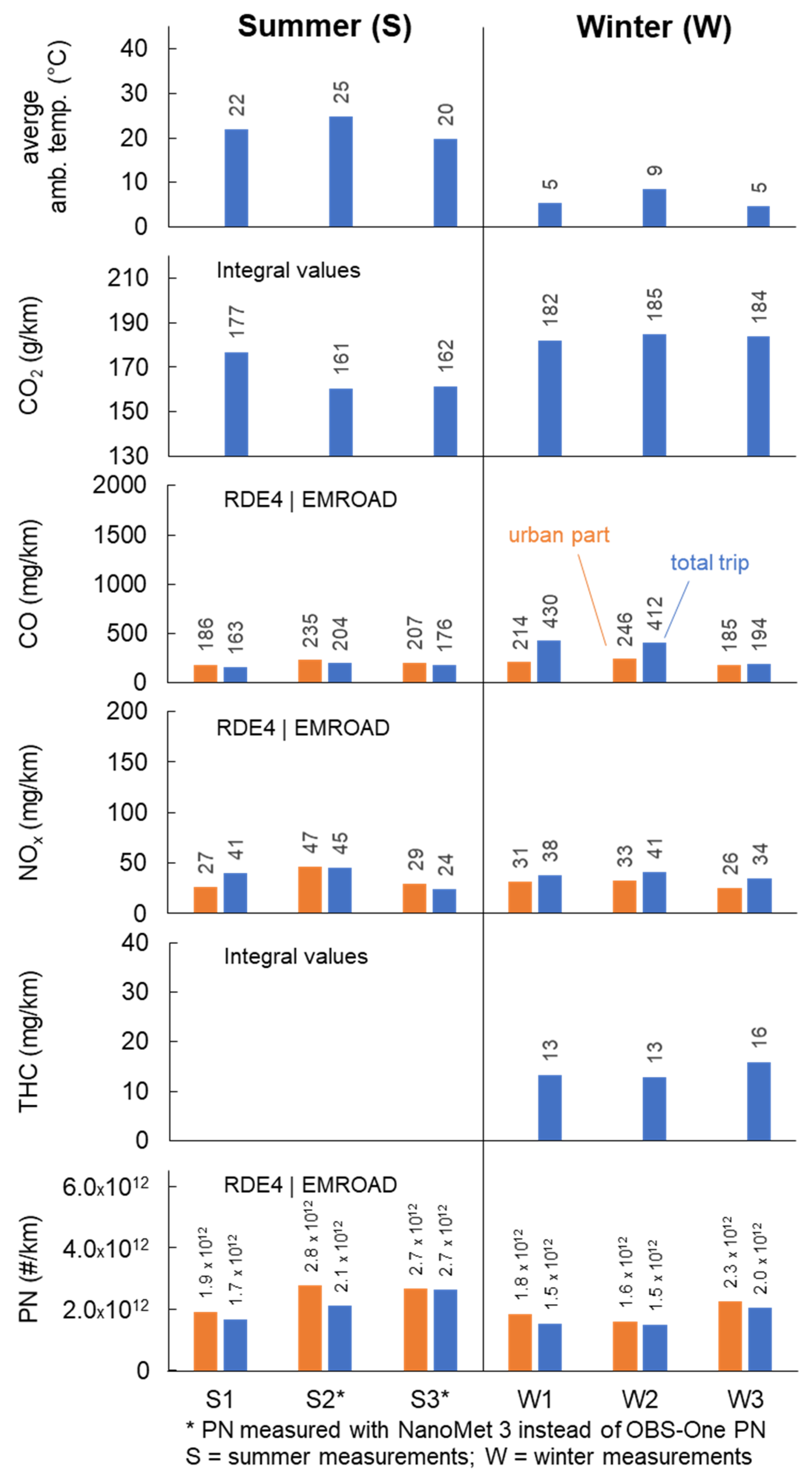
Figure 3.
Example of cumulated emissions of the diesel, vehicle 2, in summer with DPF regeneration, official RDE route.
Figure 3.
Example of cumulated emissions of the diesel, vehicle 2, in summer with DPF regeneration, official RDE route.
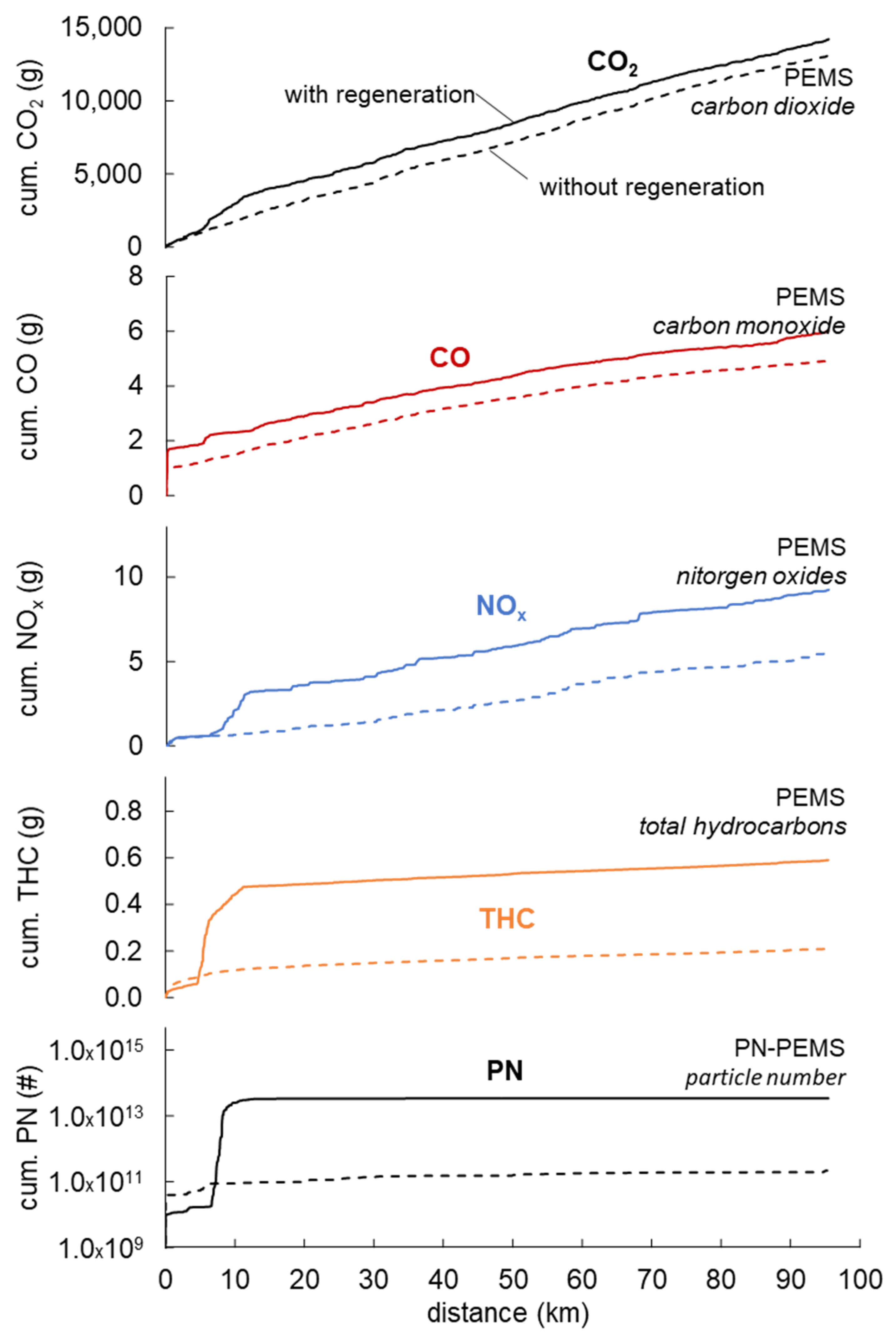
Figure 4.
Comparison of real driving emissions in summer and winter conditions, official RDE route, integral average values, vehicle 2, diesel.
Figure 4.
Comparison of real driving emissions in summer and winter conditions, official RDE route, integral average values, vehicle 2, diesel.

Figure 5.
Influences of mild and dynamic driving styles on RDE trip validity for RPA and 95th percentile of v × apos, vehicle 1, gasoline, and vehicle 2, diesel.
Figure 5.
Influences of mild and dynamic driving styles on RDE trip validity for RPA and 95th percentile of v × apos, vehicle 1, gasoline, and vehicle 2, diesel.

Figure 6.
Influences of the driving style on CO2 emissions for normality check for vehicle 1, gasoline, and vehicle 2, diesel.
Figure 6.
Influences of the driving style on CO2 emissions for normality check for vehicle 1, gasoline, and vehicle 2, diesel.
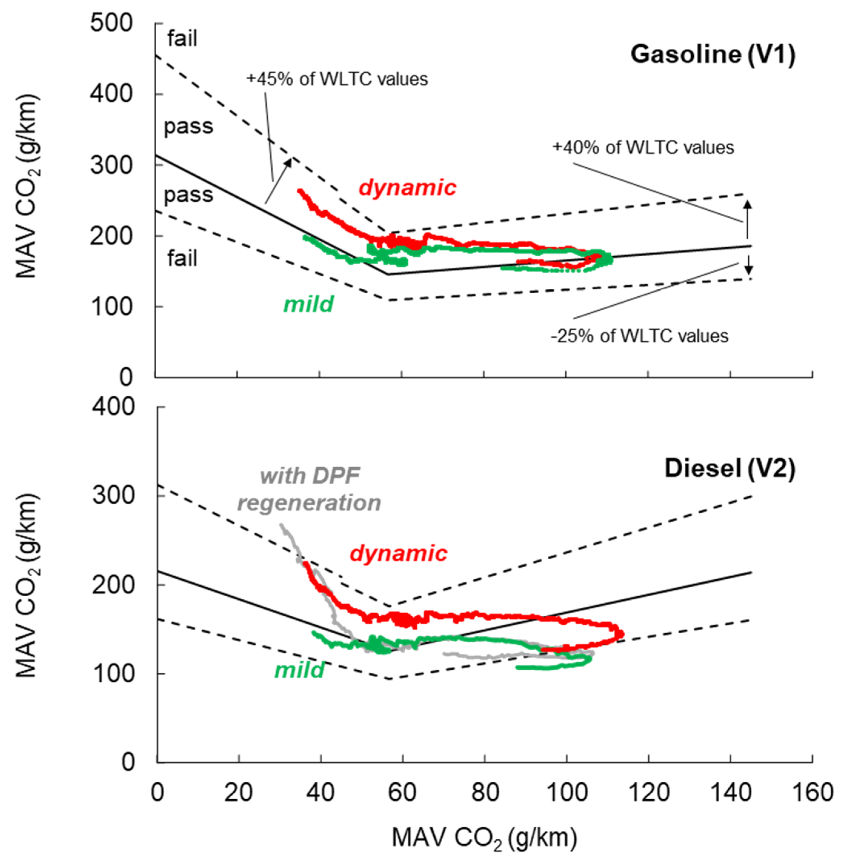
Figure 7.
Influences of the driving style on the cumulated emissions of the gasoline vehicle (V1).

Figure 8.
Influences of the driving style on the cumulated emissions of the diesel vehicle (V2).
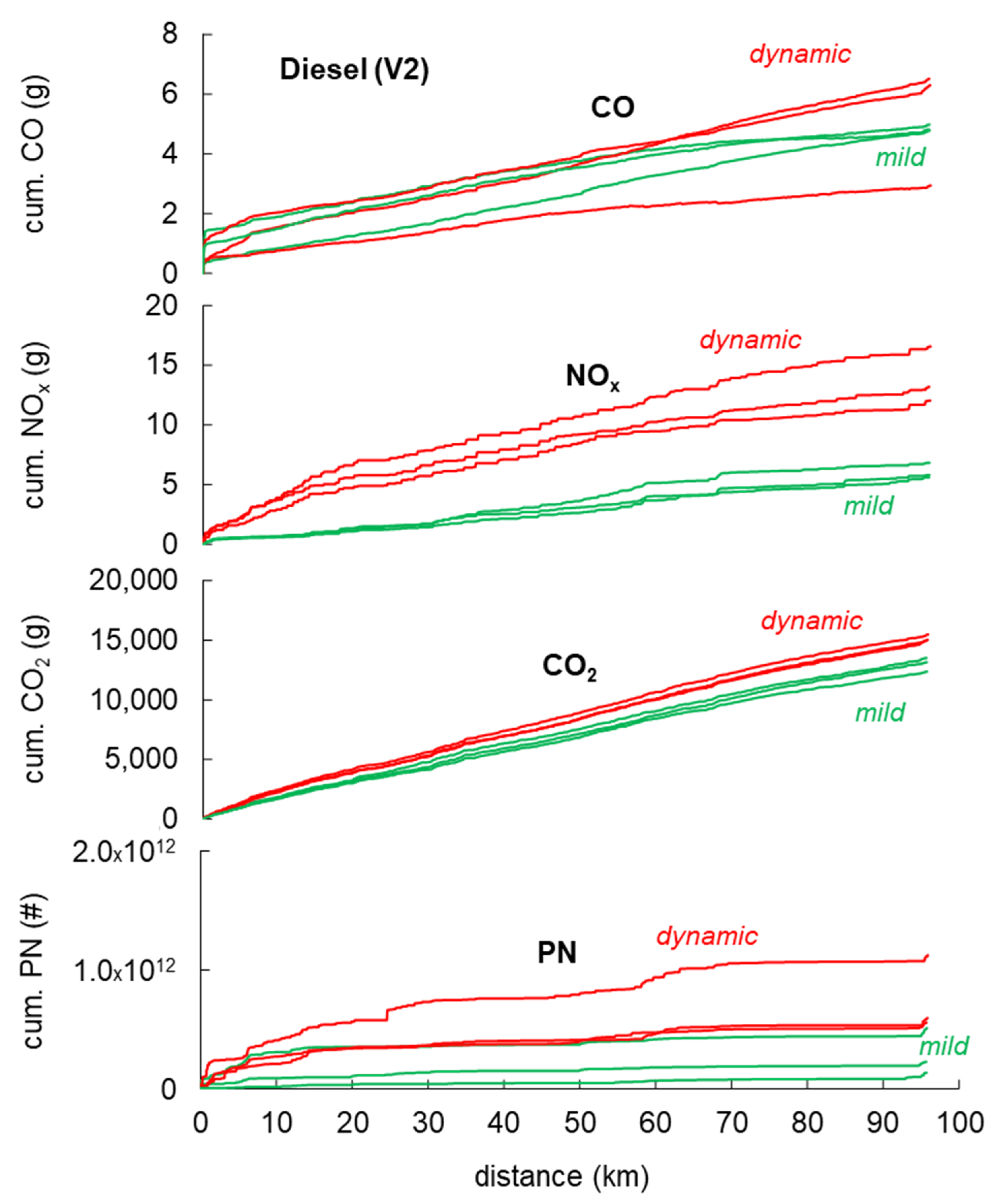
Figure 9.
Variations of RDE between the mild and the dynamic driving styles, vehicle 1, gasoline and vehicle 2, diesel.
Figure 9.
Variations of RDE between the mild and the dynamic driving styles, vehicle 1, gasoline and vehicle 2, diesel.

Figure 10.
Speed and altitude profiles of the used test circuits: cir1-standard route, cir2-high slope, cir3-high altitude, gasoline (V1).
Figure 10.
Speed and altitude profiles of the used test circuits: cir1-standard route, cir2-high slope, cir3-high altitude, gasoline (V1).

Figure 11.
Influence of the varying altitude and slope on the trip validity, gasoline (V1).
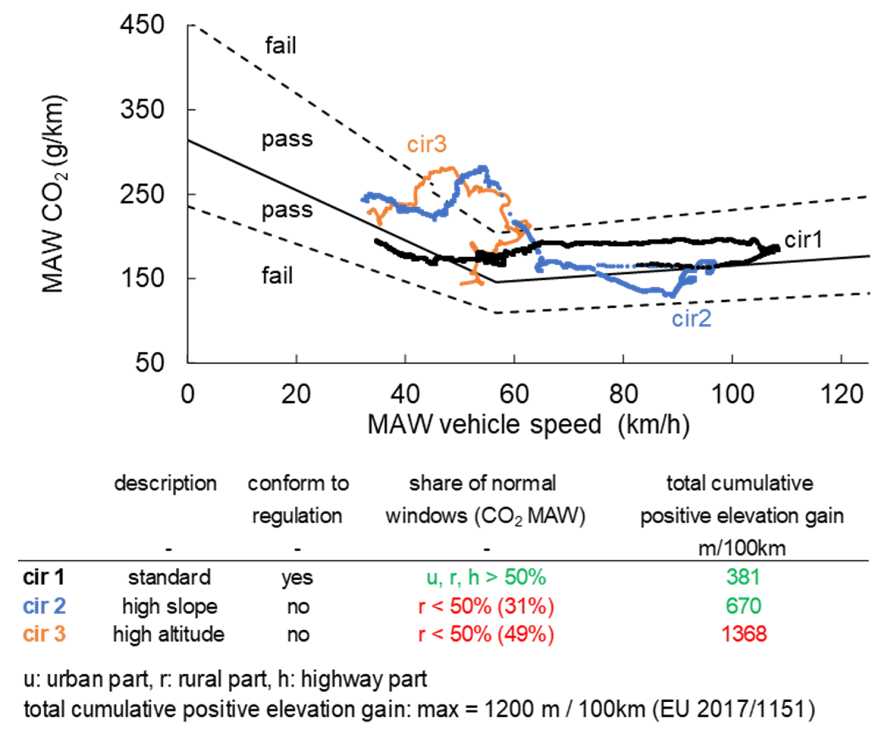
Figure 12.
Influences of high altitude and altitude variations on the cumulated emissions, gasoline (V1).
Figure 12.
Influences of high altitude and altitude variations on the cumulated emissions, gasoline (V1).
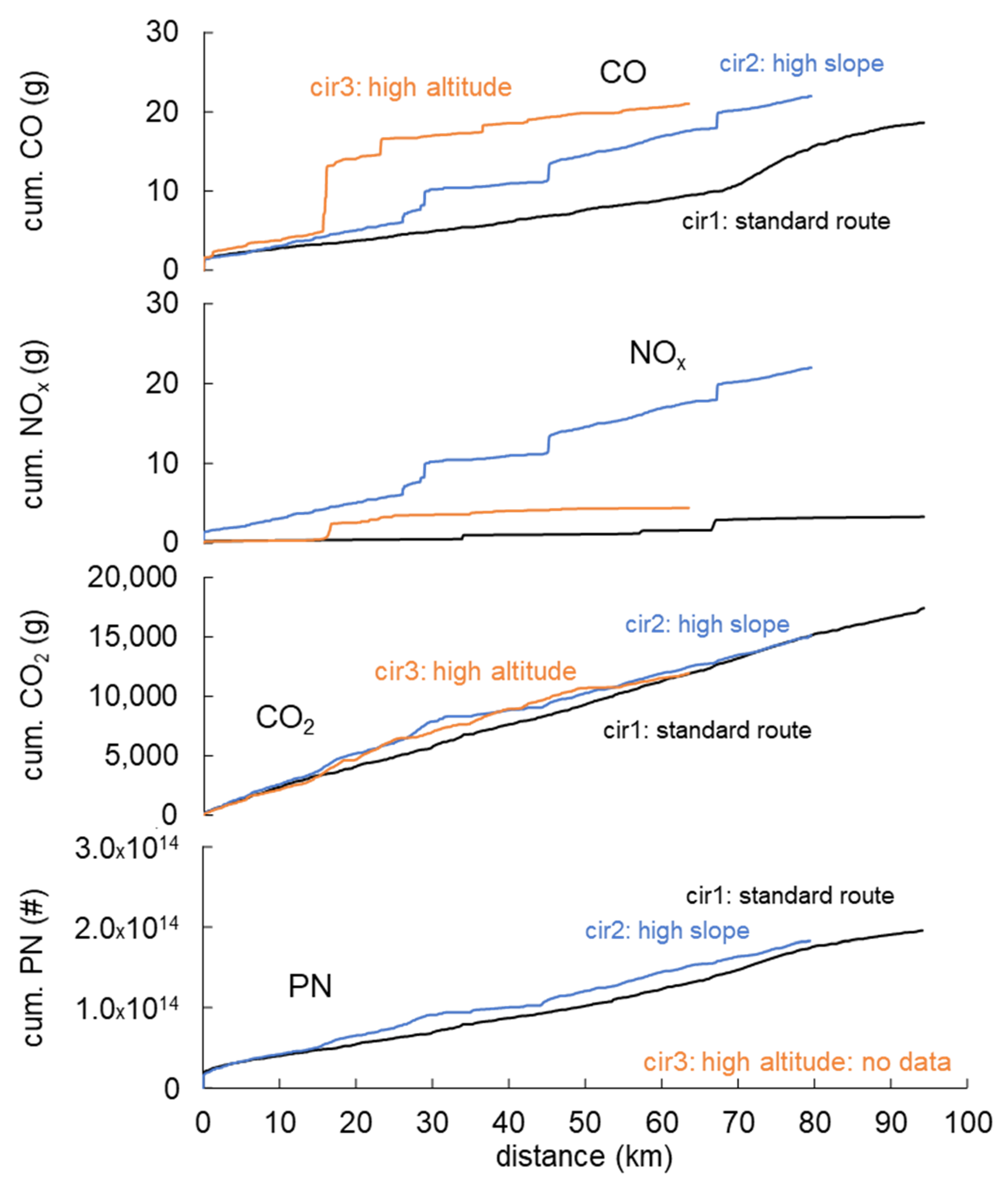
Figure 13.
Selection of characteristic circuit segments for better visualization of influences of altitude and altitude variations.
Figure 13.
Selection of characteristic circuit segments for better visualization of influences of altitude and altitude variations.
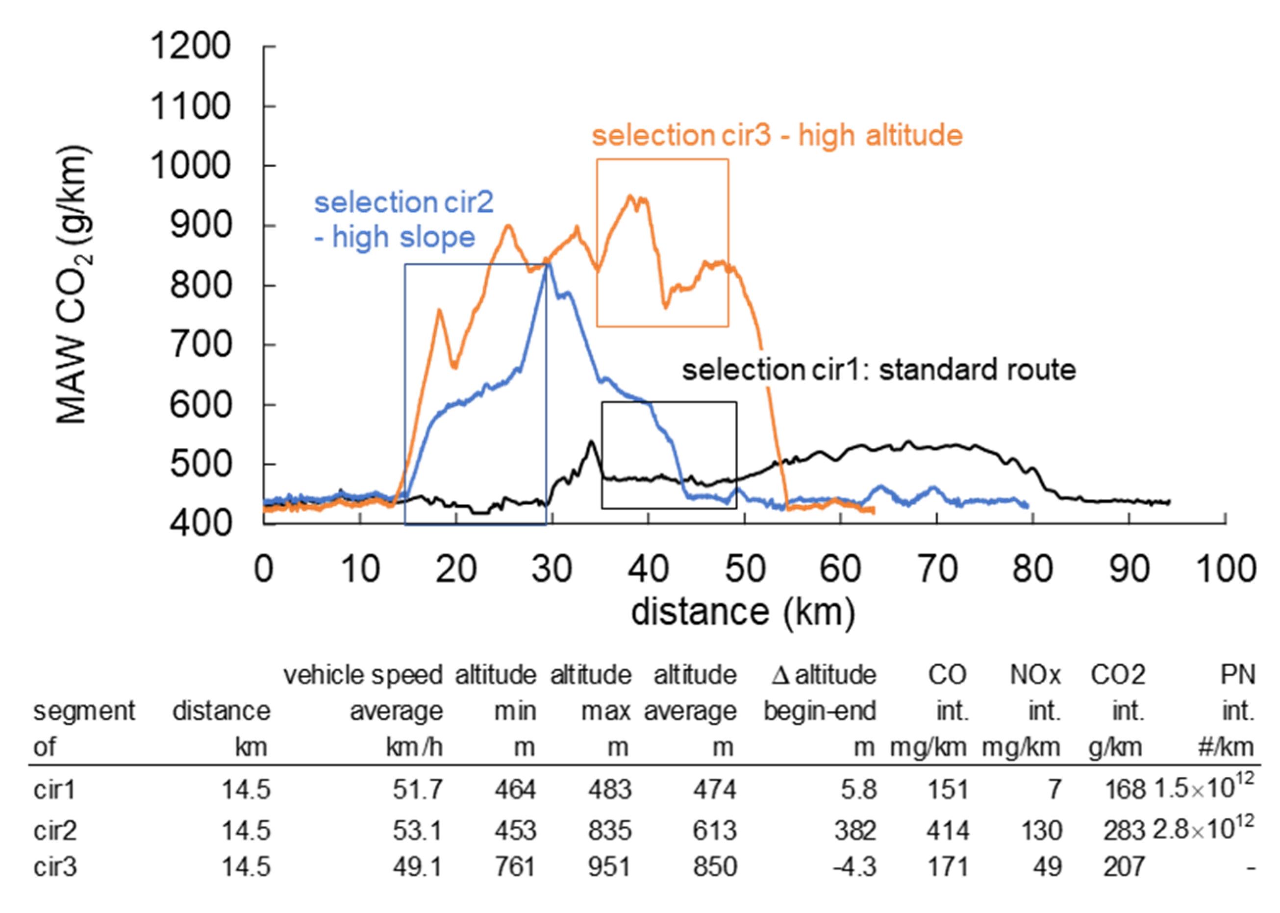
Figure 14.
Influences of slope and altitude on the cumulated emissions in the selected parts of the test circuits, gasoline (V1).
Figure 14.
Influences of slope and altitude on the cumulated emissions in the selected parts of the test circuits, gasoline (V1).

Table 1.
Data of the vehicles used for the comparison tests.
| Name | Type | Model | Fuel | EATS | Displ. | Power | ||
|---|---|---|---|---|---|---|---|---|
| - | - | Year | - | - | - | ccm | kW | |
| V1 | LDV | PC | 2012 | Gasoline | Euro 5a | 3WC | 1.596 | 132 |
| V2 | LDV | PC | 2017 | Diesel | Euro 6b | DPF + SCR | 1.968 | 110 |
Table 2.
Data of the applied GasPEMS.
| Gas PEMS | |
|---|---|
 | |
| Instruments | Horiba PEMS OBS-ONE |
| Exhaust concentrations | CO2, CO, NOx, NO2,THC |
| Measurement principle | heated NDIR *, CLD, heated line |
| Engine parameters | OBD |
| Vehicle speed and position | GPS |
| Exhaust flow | EFM |
| Ambient parameters | p, T, H |
| Electrical power | >300 W (>800 W with FID and PN) |
| Dimensions | 500 × 500 × 500 mm +Pitot tube +heated line +batteries |
* OBS one: H2O is monitored to compensate the H2O interference on CO and CO2 sample cell heated to 60 °C.
Publisher’s Note: MDPI stays neutral with regard to jurisdictional claims in published maps and institutional affiliations. |
© 2021 by the authors. Licensee MDPI, Basel, Switzerland. This article is an open access article distributed under the terms and conditions of the Creative Commons Attribution (CC BY) license (https://creativecommons.org/licenses/by/4.0/).
Share and Cite
MDPI and ACS Style
Engelmann, D.; Zimmerli, Y.; Czerwinski, J.; Bonsack, P. Real Driving Emissions in Extended Driving Conditions. Energies 2021, 14, 7310. https://doi.org/10.3390/en14217310
AMA Style
Engelmann D, Zimmerli Y, Czerwinski J, Bonsack P. Real Driving Emissions in Extended Driving Conditions. Energies. 2021; 14(21):7310. https://doi.org/10.3390/en14217310
Chicago/Turabian StyleEngelmann, Danilo, Yan Zimmerli, Jan Czerwinski, and Peter Bonsack. 2021. "Real Driving Emissions in Extended Driving Conditions" Energies 14, no. 21: 7310. https://doi.org/10.3390/en14217310
Note that from the first issue of 2016, this journal uses article numbers instead of page numbers. See further details here.