
Grid-Scale Battery Energy Storage Operation in Australian Electricity Spot and Contingency Reserve Markets


1
School of Engineering, University of Tasmania, Hobart, TAS 7001, Australia
2
SwitchDin Pty Ltd., Newcastle, NSW 2302, Australia
*
Author to whom correspondence should be addressed.
Energies 2021, 14(23), 8069; https://doi.org/10.3390/en14238069
Submission received: 19 October 2021
/
Revised: 12 November 2021
/
Accepted: 25 November 2021
/
Published: 2 December 2021
(This article belongs to the Special Issue State-of-the-Art Energy Related Technologies in Australia 2021-2022)
Abstract
:Conventional fossil-fuel-based power systems are undergoing rapid transformation via the replacement of coal-fired generation with wind and solar farms. The stochastic and intermittent nature of such renewable sources demands alternative dispatchable technology capable of meeting system stability and reliability needs. Battery energy storage can play a crucial role in enabling the high uptake of wind and solar generation. However, battery life is very sensitive to the way battery energy storage systems (BESS) are operated. In this paper, we propose a framework to analyse battery operation in the Australian National Electricity Market (NEM) electricity spot and contingency reserve markets. We investigate battery operation in different states of Australia under various operating strategies. By considering battery degradation costs within the operating strategy, BESS can generate revenue from the energy market without significantly compromising battery life. Participating in contingency markets, batteries can substantially increase their revenue with almost no impact on battery health. Finally, when battery systems are introduced into highly volatile markets (such as South Australia) more aggressive cycling of batteries leads to accelerated battery aging, which may be justified by increased revenue. The findings also suggest that with falling replacement costs, the operation of battery energy systems can be adjusted, increasing immediate revenues and moving the battery end-of-life conditions closer.
1. Introduction
Power systems traditionally rely on fossil-fuel-based generation to meet electricity demand and provide important system services that are required to keep the system in a stable state. With rising environmental concern, many countries have set targets to retire conventional generators in favour of clean and sustainable sources of energy [1,2]. As a result, wind and solar—the most abundant renewable energy resources—have been rapidly growing in their installed capacities.
Displacing traditional dispatchable generation with stochastic and unpredictable sources creates challenges in terms of ensuring reliable power-system operation and control. Renewable energy resources rarely produce the exact amount of generation required to meet electrical demand and thus require the system to keep adequate reserves to cover any fluctuations in generation or demand. Such reserves can be provided by battery energy storage systems, capable of injecting or absorbing electrical power on request almost instantaneously [3].
Various types of batteries are in different stages of maturity and are used in different applications [4]. There are several types of batteries widely used in grid-scale applications, including lithium-ion [5], lead-acid [6], redox flow [7] and molten salt (e.g., sodium-based chemistries) [8,9]. Each battery type has its unique advantages and disadvantages [10]. Due to consistent decline in prices, improved manufacturing procedures and technological innovations, most practical battery applications in recent years, both in Australia and globally, have been based on lithium-ion chemistries [5,10]. In this study, we consider lithium-ion batteries as a means to evaluate the effectiveness of our proposed battery operation framework.
Batteries have been shown to be able to support a range of power system needs, including frequency response [11,12], voltage support [13], synthetic inertia [14,15], demand peak shaving [16] and renewable generation smoothing [17,18,19]. In addition, it has been demonstrated that batteries can reduce renewable energy curtailment [20], defer transmission and distribution upgrades [21] and provide black start services [22]. Batteries can be used either in standalone application [23] or can be co-located with variable renewable energy generation [24]. Finally, battery storage can be utilized by other market participants to improve their profits or decrease their risk. Examples of various participant bidding strategies are discussed in [25,26,27]. Grid-scale battery applications have already emerged in various power systems [28].
Currently, the Australian power grid has welcomed 260 MW of battery energy storage systems (BESS) operating capacity, with the system operator expecting approximately 19 GW of combined flexible, dispatchable generation to arrive in the coming two decades [29]. Hornsdale Power Reserve, built in South Australia using 150 MW/194 MWh of Tesla batteries, provided around 15% of total mainland National Electricity Market (NEM) contingency FCAS (frequency control ancillary services) market volume in 2019 [30].
The operation of batteries heavily influences their aging [31]; an excessive number of charging/discharging cycles may significantly reduce their lifespan [32]. Battery degradation depends on factors such as depth of discharge, discharging and charging rates and overcharging or undercharging. Some researchers have accounted for degradation of battery systems participating in energy markets by placing constraints on discharge cycles [33]. Others have presented methods for including the effect of degradation on a battery’s operational cost function [34]. These different approaches to inclusion of degradation, in turn, determine the way batteries are operated, and also on their location, the value of benefits that BESS are able to yield. In this paper, we propose a framework for evaluating the effectiveness of battery participation in energy and contingency reserve markets. The main contributions of this paper can be summarized as follows:
- A mathematical model for assessing battery operation in different electricity markets (i.e., energy trading, provision of frequency regulation services), considering various control strategies, is developed.
- The battery operational cost function, based on cycling degradation, is integrated into the decision-making algorithm of the battery energy storage system.
- We investigate the value of battery participation in the electricity spot market, combined with 6-s, 60-s or 5-min raise and lower contingency markets, for the Australian National Electricity Market.
- We investigate the impact of regional generation mix on the benefits of battery participation in electricity markets, by considering battery operation in different regions dominated by particular sources of generation, such as coal, gas, hydro, wind or solar.
The paper is structured in the following way. Section 2 presents an overview of the Australian electricity market. Section 3 describes how grid-scale battery operation can be modelled and which factors influence its degradation. Section 4 provides a demonstration of how batteries can be used within the Australian electricity market. Case studies are then presented in Section 5 considering different bidding strategies and battery operation in five regional markets of Australia. Conclusions are presented in Section 6.
2. The Australian Electricity Market
Australia’s National Electricity Market supplies electricity to five state-based regional markets: Queensland (QLD), New South Wales (NSW), Victoria (VIC), Tasmania (TAS) and South Australia (SA). The states are connected by interconnectors, enabling trading of energy between adjacent geographical regions. Trading among five regional markets is managed by the Australian Energy Market Operator (AEMO) [35,36,37].
Currently, coal power plants provide most of the electricity generation in Australia, while renewables generate nearly 30% of electricity. The percentages of different sources of generation in the NEM states in 2020, along with average wholesale spot prices, are shown in Table 1 [38]. The highest renewable energy penetration is observed in Tasmania (83% hydro and 14% wind) and South Australia (17% solar and 42% wind).
The exchange between electricity consumers and producers within each regional market is facilitated through a spot energy market managed by AEMO ensuring that the instantaneous generation meets demand at all times. In order for the system to operate in a secure and reliable manner, the NEM maintains an appropriate level of reserves. Reserve trading is implemented within the ancillary service markets [39].
To obtain the operational schedule for all the market participants, a centralized dispatch engine is engaged. According to the dispatch model, both the energy and the ancillary service markets are co-optimized, resulting in the optimal trade-off between the energy and the reserve capacity allocation. In Section 2.1 we first look at the electricity spot market: the way trading is implemented, how the market is cleared and how the price is formed. The markets for ancillary services are then considered in Section 2.2. Most liberalised, market-based electricity systems operate in a similar manner.
2.1. Energy Market
Energy market operation requires AEMO to first produce forecasts of the electrical demand for each NEM region over at least the next trading day. To meet the expected demand, AEMO schedules available electricity suppliers for each dispatch interval within a trading day, according to their bids. Generators are required to submit their offers to AEMO ahead of time, indicating for each dispatch interval how much energy they could produce and the price at which they would be willing to produce it. To determine which generators will be dispatched for each interval, the market operator stacks these bids in order of rising price and schedules generators, starting from the most affordable options, followed by progressively more expensive ones. The last accepted bid, required to ensure demand is just met, determines the market price in each region. All generators within a market region receive the same market price for any dispatched energy, regardless of their bidding prices. The structure of the Australian National Electricity Market (NEM) is shown in Figure 1.
Depending on their bids, generators are dispatched for each 5-min dispatch interval. Prior to 1 October 2021, the market price for each 30-min trading interval was set by averaging the price of six dispatch intervals (Figure 2) [35]. However, after 1 October 2021, the trading interval is the same as the dispatch interval (i.e., 5-min), and the trading and dispatch interval prices are the same [40].
The Australian electricity market treats the energy spot market as part of a day-ahead market. All market participants are required to submit their bids for the next day, for each trading interval between 4 A.M.–4 A.M. the following day, prior to 12.30 P.M. each day. During the trading day, participants can submit rebids, which can adjust the volume of the approved energy bid but cannot change the bidding price. Rebids can be submitted any time before the start of the relevant dispatch interval.
2.2. Reserve Markets
Maintaining system reserves is important for secure and reliable operation of the electrical power system. In Australia, reserves are procured through the frequency control ancillary services (FCAS) markets. There are eight separate markets for delivering FCAS, described in Table 2 [41,42].
A conceptual illustration of fast, slow and delayed contingency responses is presented in Figure 3. The fast response arrests the immediate rise or fall of frequency. The slow response stabilizes the system frequency. The delayed response enables the frequency recovery back to the normal operating band (NOB).
It is important to outline the difference between enablement and delivery of contingency services. The latter is a physical provision of energy into the power system in response to a contingency event actually taking place, while the former refers to the capacity that is reserved for provision in the unlikely event of the contingency occurring. Participants in the contingency FCAS market are paid for the enablement of the service, regardless of whether energy is provided. The FCAS transactions are settled according to the clearing-price difference for each of the FCAS markets and calculated as follows:
where MWE is the amount of MWs enabled for particular FCAS market and CP is the clearing price. Division by 12 is used to convert the MWE’s unit (MW for 5 min) into MWh to match the units of clearing price–dollars per MW per hour (MW of reserve enabled for an hour) [41].
3. Grid-Scale Battery Energy Storage
3.1. The Role of Batteries in Electricity Markets
A battery energy storage system can be used to provide electrical power to the grid by discharging or absorb power from the grid by charging, thus enabling batteries to participate in energy markets both as a generator and as a load (Figure 4). Due to their fast-ramping capabilities, batteries can be quite effective in the provision of system reserves, when some part of their charging/discharging capacity is reserved and can be requested by system operators at any time. When participating in contingency reserve markets, BESS must initiate the response (adjusting the active power output) when the local frequency deviates away from the normal operating frequency band [42]. In this paper, we focus on battery operation in a wholesale energy market and in several contingency reserve markets.
Power system contingency events are rare, but severe disturbances require near-instantaneous response from units enabled by the market operator. To provide contingency reserve services, BESS would be required to be capable of reacting fast enough to provide the contracted power within the specified time interval. Even though such responses may result in some battery wear, over a long period of time (one year), these infrequent battery engagements can be neglected since they will be small in number and duration compared to normal battery cycling for energy applications. An example of battery response to a contingency event is presented in Figure 5, where some capacity is engaged during an over-frequency event (at 13.35) and an under-frequency event (at 14.05).
3.2. Battery Health Characteristics
For a generic lithium-ion battery (the chemistry widely used in grid-scale power system applications [5,45]), there are different factors that might result in battery-cell degradation. These factors can be non-operational or operational in nature. Non-operational factors include ambient temperature, air humidity and calendar (shelf) degradation; they are independent of battery operation. Operational factors are very sensitive to the way the batteries are used and depend on the following parameters:
- Battery-cell temperature. There is an exponential decay in battery life expectancy with increased BESS operating temperature. Extremely high temperatures can lead to the build-up of internal pressure, battery bursts and fire hazards. To prevent such events from happening, BESSs are generally equipped with climate-control systems that maintain battery-cell temperature at a constant value.
- Battery charge and discharge rate. The metric used to measure the battery discharge rate is called the ‘C’ rate, where the battery discharging at rate 1C would be fully discharged in one hour. A battery discharging at higher rates (e.g., 2C) would fully discharge faster (half an hour for 2C, quarter of an hour for 4C, etc.). Degradation occurring at lower ‘C’ rates is generally gradual, while increasing rates result in an exponential rise in degradation [34]. The discharging rate can be included as an additional cost component within the battery cost function that can be used as a metric to determine if aggressive battery operation is cost-effective in a given market environment. In practice, however, it is not recommended to operate batteries above their recommended ‘C’ ratings because the resultant temperature rise would result in additional cooling costs or increase the risk of fire.
- Battery-cycle depth of discharge. One of the most important parameters affecting battery degradation is the depth to which the batteries get discharged during each cycle of operation. The dependency between the depth of discharge (DOD) and degradation is non-linear. For example, a generic lithium-ion battery can perform around 22,000 cycles of 30% to reach its end-of-life conditions. However, if the cycle depth is increased to 80%, the battery would only perform 3000 cycles.
- Over-charge, under-charge and average state of charge. Extreme values of state of charge (SOC) can significantly damage the battery health [46]. Therefore, to avoid such events, several constraints are enforced on minimum, maximum and average values of SOC.
3.3. Degradation Cost Function
There are many ways to include operational degradation within BESS decision-making algorithms. Some researchers choose to explicitly constrain battery operation in order to mitigate unwanted battery wear [33]. Others attempt to include degradation parameters as separate components within the battery operational cost function [34].
In this paper, we present a framework to evaluate the benefit of BESS operation in different electricity markets. For illustrative purposes, we consider unconstrained battery operation and compare it with battery operation based on the degradation model presented in [47]. According to this model, batteries undergo a certain degradation after each charge-discharge cycle of specified depth . Operational costs are evaluated for each cycle, i ∈ I, where is the set of all cycles, as follows:
- Depth of discharge () of the considered cycle, i, is estimated.
- Life loss (associated with the cycle, i, corresponding to the % of total-cycle life reduction, is estimated. It has a dependence on and is expressed as [34]:where and are coefficients capturing the relationship between life loss and the cycle depth, which may be determined empirically for a given class of battery.
- The marginal cost of that cycle, i (), is evaluated by prorating the battery replacement cost, , to the incremental life loss:
In order to find the depth of each cycle, the rainflow counting algorithm is used [48]. An example of using the rainflow algorithm is presented in Figure 6, where three cycles of depth, 20%, 50% and 10%, respectively, are detected, along with two half cycles of depth 60% (one discharging and one charging half cycle). It is assumed that to evaluate battery degradation, only full cycles and discharging half cycles need to be considered [47].
The rainfall counting algorithm is a good ex-post method that can be used as a benchmark to calculate the degradation that a battery has experienced over some period of time. Due to its non-linear characteristics, it is hard to integrate the algorithm within an optimization problem. According to [47], we can assume that battery degradation occurs only during the discharging phase and that the cycle depth for the cycle occurring at time t can be represented as a function of discharging power at time t, :
and
where and are the battery discharging efficiency and rated energy capacity. The incremental life loss ( owing to the incremental cycle depth can be expressed as:
Rearranging (6)
With being the duration of a dispatch interval (e.g., 1/12 for a market cleared every 5 min), the energy change over one dispatch interval:
Therefore:
or
For Equation (10) to be included into the optimization problem, can be replaced with segment gradients (for segments 1 … J) of a piecewise linearized life-loss function corresponding to (2), under the following assumptions:
For a given dispatch interval, of duration
- is battery discharge power, is battery charge power, and these are fixed for the entire interval.
- Energy is discharged/charged from the battery and can be considered to come from one or more segments of the cycle life-loss function, depending on the amount of stored energy assigned to those segments.
- Total discharge cost of a dispatch interval is minimized to ensure cycle degradation is accurately accounted for (since cycle loss is a function of DOD for a cycle, not SOC).
As result, the sum of discharged energy from all segments equals the total discharged energy from the battery and is expressed as:
Each segment can be charged or discharged, where the total power coming from the battery is equal to the sum of discharged power fractions coming from each segment:
Each segment has a discharge cost (fixed value for each segment). It can be obtained by dividing the full depth of discharge range (0% to 100%) into J segments:
where the marginal cost of discharging, , measured in $ per MW of discharge, is determined, according to which segment, j, the current cycle depth corresponds to, in turn calculated from the marginal cost of discharge for that segment, :
The total cost for each dispatch interval, t, is evaluated as:
4. Model for Assessing the Battery Energy Storage System Operation
To evaluate battery operation within different markets, under the assumption that it is small enough that it acts as a price-taker participant and will not influence prices, an optimization problem is solved. A formal description of this optimization requires definition of the following parameters:
- —the number of time intervals, each denoted by t, included in the optimization horizon (e.g., for 24 h horizon with 5 min dispatch intervals, T = 288);
- —the number of segments, each denoted by j, in the BESS cycling cost function;
- —duration of a dispatch interval, e.g., 1/12 for a market cleared every 5 min (hours);
- —forecast price on the energy wholesale market ($/MWh);
- —forecast prices on 6 s, 60 s and 5 min raise FCAS markets ($/MWh);
- —forecast prices on 6 s, 60 s and 5 min lower FCAS markets ($/MWh);
- —charging and discharging efficiencies (%);
- —energy limits of BESS (MWh);
- —maximum amount of energy stored in cycle-depth segment j (MWh);
- —initial amount of energy stored in cycle-depth segment j of BESS at the beginning of the optimization horizon (MWh);
- —energy stored in the battery at the last interval (T) of the optimization horizon (MWh);
- —maximum charging and discharging power limits of BESS (MW)
Decision variables (positive real numbers unless stated otherwise) are also defined as:
- —discharging power of the BESS at time interval t (MW);
- —charging power of the BESS at time interval t (MW);
- —available discharging power of the BESS for reserve provision at time interval t (MW);
- —available charging power of the BESS for reserve provision at time interval t (MW);
- —the quantity of reserve power enabled for 6 s, 60 s and 5 min raise FCAS markets, respectively (MW);
- —the quantity of reserve power enabled for 6 s, 60 s and 5 min lower FCAS markets, respectively (MW);
- —binary variable equal to 1 if the BESS provides reserve at time interval t and equal to 0 otherwise;
- —binary variable equal to 1 if battery is charging and 0 otherwise;
- —energy stored in cycle-depth segment j of the BESS at time interval t (MWh);
- —charging BESS power for cycle-depth segment j at time interval t (MW)
- —discharging BESS power for cycle-depth segment j at time interval t.
The objective of the BESS scheduling algorithm is to maximize revenue from participation in the electricity energy and FCAS markets, while considering the BESS operational costs. The objective function of the BESSs participating in all relevant markets of Australia can be defined as follows:
where is the revenue obtained from performing price arbitrage–buying electricity at a lower price and selling it when the price is higher. Arbitrage revenues are computed as follows:
where is the revenue from participating in the raise reserve contingency market, including the 6 s, 60 s and 5 min responses to frequency fall via FCAS markets. Revenues from raise FCAS are computed as follows:
where is the revenue from participating in the lower reserve contingency market, including the 6 s, 60 s and 5 min responses to frequency rise via FCAS markets. Revenues from lower FCAS are computed as follows:
The BESS operational costs depend on the utilized degradation model. With the degradation model described in Section 3.3, the battery operational costs are computed as:
The optimization is subject to the following constraints:
Constraint (21) ensures that the total BESS charging power at time interval equals the sum of charging powers in each battery segment, , at time interval . Constraint (22) is similar to (21) but for discharging powers.
Constraints (23) and (24) use binary element , which prevents simultaneous charging and discharging of a battery.
Equation (25) enforces the consistency and continuity of charging/discharging characteristics for each segment of the battery (the energy stored in the BESS segment on the next time interval equals the value on the previous interval plus the power injected into the BESS segment, minus the power withdrawn from this segment and minus efficiency losses).
Constraint (26) enforces the maximum limit of energy that can be stored in each BESS segment.
Constraint (27) enforces minimum and maximum limits of battery state of charge.
Constraints (28) and (29) allow initial and final values for the energy content to be set in the BESS for the current optimization.
Constraints (30)–(38) must be included when the BESS participates in reserve markets. Constraint (34) states that if the battery sells the power to the grid at time t, less battery capacity can be reserved for raise contingency markets. Constraint (35) is similar to (34) but is related to the lower contingency market. Constraints (37) and (38) enforce that the battery has enough energy to sustain the frequency response for 60 s, 5 min and 10 min when participating in the 6 s, 60 s and 5 min FCAS markets, respectively.
The presented optimization problem is solved for each trading day using a 24-h forecast. For demonstration purposes, the forecast is assumed to be perfect. The problem is solved using the GUROBI mixed integer linear programming solver within the MATLAB environment [49]. The total BESS revenue from participation in electricity markets and costs associated with battery cycling are evaluated over a one-year operational period.
5. Case Studies
5.1. Battery Description and Model Assumptions
The battery used for all case studies presented in this paper is specified in Table 3, corresponding to [47] battery system. Battery degradation is assumed to follow the model described in Section 3, fitted to the specified battery-cycle life as a function of depth of discharge. Energy spot and FCAS prices for the Australian market are sourced from AEMO, corresponding to a one-year period (2020) [50]. The battery is considered to participate in the market as a price-taker, meaning that its activity in the market would be of a small volume, such that it does not have sufficient market power to influence prices. At the same time, the battery would be large enough to be registered by the market operator for provision of ancillary services (>1 MW). We consider only the revenue from participation in the energy spot market and from enablement of ancillary services. Revenue from the actual delivery of contingency service, which can be assumed to be very small, is not included in this study.
According to battery specifications, higher values of battery depth of discharge result in reduced cycle life. For example, if the BESS of Table 3 performs 3000 cycles at 80% DOD, the battery would reach its end-of-life condition (i.e., would “lose” 100% of its usable capacity). In order to evaluate the life-cycle loss obtained after one cycle at 80% DOD, we can divide the total battery life (i.e., 100%) by the rated number of cycles (i.e., 3000). The same procedure can be done for the whole range of cycle depths, resulting in the life-cycle loss function presented in Figure 7 and fitted into the function (2):
In addition, we assume that the cells comprising the battery pack are identical and would age simultaneously. It is assumed that the battery would be replaced at its end-of-life condition (when battery reaches its shelf or cycle end life, whichever comes first). Therefore, the battery life expectancy, for a given cycle depth, , is obtained as follows:
Since in these case studies, we evaluate revenue over a finite period only (one year), evaluating battery life expectancy based on how the battery has been cycled over that period provides us with an objective means of comparing the impact of different charge/discharge strategies on overall battery longevity.
5.2. Battery Operation Considering Different Bidding Strategies
In this section, we consider three BESS bidding strategies (Table 4). We consider one year of market operation only, and to highlight the differences between strategy outcomes, we focus on one regional market: NSW.
Strategy 1 enables BESS operation that maximizes the revenue from trading energy on a spot market. This is a partial solution to the optimization problem presented in Section 4, where terms (9–11) are omitted. Unconstrained by cycling costs, the battery tries to capture any opportunity for price arbitrage, resulting in aggressive BESS cycling.
For illustrative purposes, one day of battery operation under Strategy 1, chosen at random, is provided. Figure 8 shows energy and FCAS prices across the day, while Figure 9 shows the corresponding battery actions and resulting SOC. During this single day, the battery performs three equivalent cycles at 80% DOD, corresponding to 0.1% degradation, with frequent transitions between charge and discharge, even for small price differentials.
Strategy 2 enables BESS operation that maximizes the combined revenue from trading on both energy spot and contingency FCAS markets. To more clearly highlight the impact of operating on both energy and reserve markets, only a single reserve market (the most profitable one in NSW—6 s raise [51]) is included first. Instead of responding to any significant but small variation in energy price, the BESS keeps some capacity reserved for provision of ancillary service. This prevents excessive battery cycling, provided reserve markets are valuable enough. For the same single-day example (Figure 8), the battery now performs 1.16 equivalent cycles at 80% DOD, corresponding to 0.04% degradation (a 2.5 times degradation improvement compared to strategy 1), as in Figure 10.
Strategy 3 enables BESS operation based on the degradation cost function (described in Section 3) and simultaneous participation in both energy spot and 6 s raise FCAS markets. Under such a strategy, optimal operation of the BESS can be achieved, with the battery responding only to energy price variations that will yield revenue greater than what the corresponding loss of battery life is valued at, otherwise reserving its capacity for the FCAS market. During the same single-day example, the battery now barely cycles at all (as shown in Figure 11), since the energy price differential is insufficient to warrant it and because FCAS revenue can be extracted instead.
Table 5 summarizes BESS performance over the one-year operational period for the NSW market using the three abovementioned strategies. Market revenues, battery cycling costs, battery degradation and battery life expectancy are calculated and compared for each strategy. Battery degradation is calculated using the ex-post benchmark method, the rainflow counting algorithm. The cost of cycle aging is calculated using (3). Battery life expectancy is calculated using (39). The breakdown of revenues and costs associated with each strategy is presented in Figure 12.
Highest revenues from the energy market are observed when the first strategy is applied. This is achieved by aggressively cycling the battery (913.6 equivalent cycles), resulting in high degradation (30%) and a decrease in life expectancy (3 years instead of 10). When the battery is introduced to FCAS markets (under Strategy 2), additional revenues are generated by reserving some of the battery capacity for the provision of ancillary services. As a result, the battery participates less in the energy market, experiencing lower degradation (21%) and extending its life expectancy (to nearly 5 years). Under the third strategy, the battery is operated considering cycling costs, where it responds only to significant variations in energy prices, otherwise reserving its capacity for FCAS markets. As seen from the results, the battery degrades by only 1.21%, with insignificant compromise to its life.
5.3. Optimal Battery Operation in State-Based Regional Markets of the NEM
In this Section, we consider the BESS operation in different regional markets of Australia, where, based on Strategy 3, the battery can select how much of its capacity to allocate to the energy or a particular FCAS market.
An illustration of battery operation using Strategy 3 in all six FCAS markets, alongside the spot market, is presented in Figure 13. It can be seen that the fast (6 s) FCAS market is favoured by the BESS over the slow and delayed FCAS markets. This can be explained by the following factor: prices in the fast FCAS market are generally higher. Additionally, in slow and delayed markets, the BESS system has to reserve more capacity to be able to provide a response for the longer timeframes if needed (i.e., 5 and 10 min, respectively, compared to 60 s for the fast FCAS market).
Results for one year of BESS operation in the five state-based regional markets in the NEM are presented in Figure 14. When the same battery is placed in different markets, the similar trend of favouring the 6 s raise FCAS market is observed. In South Australia (SA), however, the state in which revenues from all FCAS markets are generally much higher, the 6 s lower market can also generate considerable revenue. The high price variability observed in NSW results in substantial involvement of the BESS in the energy spot market. In this case, the revenue gained from performing price arbitrage is almost equal to the revenue obtained from contingency reserve markets. At the same time, the BESS governed by the Strategy 3 is less cycled, and therefore, costs are insignificant. SA, with its high share of intermittent generation (17% solar and 42% wind, on average, across the year), presents greater opportunities in all FCAS markets compared to other states. Tasmania, a state highly dependent on hydro power plants (83% hydro generation) and with frequently high levels of import/export via an asynchronous HVDC interconnector, may often lack sufficient responsive generation, thus resulting in high 6 s FCAS prices. NSW, the state with high price volatility and frequent high energy prices, presents some opportunities for energy arbitrage. At the same time, predominantly supplied by steam-driven generation, NSW experiences an abundance of fast-acting resources, resulting in generally low FCAS prices.
6. Conclusions
A framework to evaluate the effectiveness of battery participation in different energy and reserve markets under different conditions (tracking various objectives or considering different battery degradation models) was developed. The proposed framework was applied to the Australian National Electricity Market. It was demonstrated that if grid-scale batteries are utilized in the electricity market only, revenues from energy arbitrage can be largely offset by cycling degradation costs, unless some suitable mechanism is also implemented in order to prevent costly arbitrage occurring on small market-price differentials. By allowing the battery to participate in ancillary service markets, additional revenue can be generated, while also preventing unprofitable arbitrage cycling. Optimal battery operation, meanwhile, can only be achieved when cycling costs are included directly in the decision-making algorithm—in our case, as an additional cost component in the objective function. In such a case, the battery was shown to respond only to significant variation in prices, otherwise reserving its capacity for markets of ancillary services. Participating in contingency reserve markets (e.g., optimally selected from six types available in Australia), batteries were shown to significantly increase their revenues without compromising their life expectancy.
In each of the five regional Australian markets, the fast raise frequency control ancillary market presented considerably higher revenue compared to other types. It was demonstrated that markets in regions with high penetration of intermittent resources (wind and solar), like South Australia, are highly volatile and can generate the highest revenue in almost all contingency markets. In regions such as Tasmania, relying predominantly on hydro power and with significant levels of HVDC import and export, a lack of fast-responding generation can result in high prices for fast contingency service provision, thus providing batteries with the opportunity to generate significant revenues. In markets where conditions result in high price volatility and frequently high energy prices (such as experienced in NSW in 2020), participation in reserve markets can be partially displaced by involvement in energy trading, with battery cycling degradation justified by the additionally generated revenue. In general, smaller contingency reserve market opportunities can be observed in systems that have large amounts of conventional thermal generation, where an abundance of fast-acting synchronous generation resources dictates low prices in ancillary services markets (e.g., in Queensland, Victoria and New South Wales).
The analysis presented in this work demonstrates that significant net benefit can be accrued by batteries if they participate wisely in wholesale energy and reserve markets. With greaterer benefits being associated with market regions where renewable resources make up a greater share of the market, this suggests that the continued deployment and participation of battery systems in markets is likely to continue as power systems transition away from carbon-intensive sources of generation.
Future research should consider the potential impact of battery characteristics on battery operation in electricity and reserve markets. It would be beneficial to consider what value batteries can realise from participating in regulation reserve markets and how this would be reflected in battery degradation. Finally, with the introduction of a large number of grid-scale battery storage systems, issues related to market saturation become particularly relevant, when profit seeking behaviour of battery owners would impact the profitability of other participants.
Author Contributions
Conceptualization, E.B., M.N. and E.F.; formal analysis, E.B.; methodology, E.B., M.N. and E.F.; resources, A.W.; software, E.B.; supervision, M.N. and E.F.; visualization, E.B. and A.W.; writing—original draft, E.B.; writing—review and editing, M.N., E.F. and A.W. All authors have read and agreed to the published version of the manuscript.
Funding
This research received no external funding.
Institutional Review Board Statement
Not applicable.
Informed Consent Statement
Not applicable.
Data Availability Statement
Data supporting reported results is available on request.
Acknowledgments
The authors would like to acknowledge Alex Radchik from SwitchDin Pty Ltd. for contributions to this paper and for valuable advice.
Conflicts of Interest
The authors declare no conflict of interest.
Abbreviations
The following abbreviations are used in this manuscript:
| AEMO | Australian Energy Market Operator |
| BESS | Battery Energy Storage System |
| DOD | Depth of Discharge |
| FCAS | Frequency Control Ancillary Services |
| HVDC | High-Voltage Direct Current |
| NEM | National Electricity Market |
| NOB | Normal Operating Band |
| NSW | New South Wales |
| PV | Photovoltaics |
| QLD | Queensland |
| SA | South Australia |
| SOC | State of Charge |
| TAS | Tasmania |
| VIC | Victoria |
References
- Ajadi, T.; Cuming, V.; Boyle, R.; Strahan, D.; Kimmel, M.; Logan, M. Global Trends in Renewable Energy Investment 2020; Frankfurt School of Finance & Management: Frankfurt am Main, Germany, 2020. [Google Scholar]
- Gielen, D.; Boshell, F.; Saygin, D.; Bazilian, M.D.; Wagner, N.; Gorini, R. The role of renewable energy in the global energy transformation. Energy Strategy Rev. 2019, 24, 38–50. [Google Scholar] [CrossRef]
- He, G.; Chen, Q.; Kang, C.; Xia, Q.; Poolla, K. Cooperation of wind power and battery storage to provide frequency regulation in power markets. IEEE Trans. Power Syst. 2016, 32, 3559–3568. [Google Scholar] [CrossRef]
- Argyrou, M.C.; Christodoulides, P.; Kalogirou, S.A. Energy storage for electricity generation and related processes: Technologies appraisal and grid scale applications. Renew. Sustain. Energy Rev. 2018, 94, 804–821. [Google Scholar] [CrossRef]
- Chen, T.; Jin, Y.; Lv, H.; Yang, A.; Liu, M.; Chen, B.; Xie, Y.; Chen, Q. Applications of lithium-ion batteries in grid-scale energy storage systems. Trans. Tianjin Univ. 2020, 26, 208–217. [Google Scholar] [CrossRef] [Green Version]
- McKeon, B.B.; Furukawa, J.; Fenstermacher, S. Advanced lead–acid batteries and the development of grid-scale energy storage systems. Proc. IEEE 2014, 102, 951–963. [Google Scholar] [CrossRef]
- Perry, M.L.; Weber, A.Z. Advanced redox-flow batteries: A perspective. J. Electrochem. Soc. 2015, 163, A5064. [Google Scholar] [CrossRef]
- Andriollo, M.; Benato, R.; Sessa, S.D.; di Pietro, N.; Hirai, N.; Nakanishi, Y.; Senatore, E. Energy intensive electrochemical storage in Italy: 34.8 MW sodium–sulphur secondary cells. J. Energy Storage 2016, 5, 146–155. [Google Scholar] [CrossRef]
- Sessa, S.D.; Palone, F.; Necci, A.; Benato, R. Sodium-nickel chloride battery experimental transient modelling for energy stationary storage. J. Energy Storage 2017, 9, 40–46. [Google Scholar] [CrossRef]
- Bowen, T.; Chernyakhovskiy, I.; Denholm, P.L. Grid-Scale Battery Storage: Frequently Asked Questions; National Renewable Energy Laboratory (NREL): Golden, CO, USA, 2019. [Google Scholar]
- Pusceddu, E.; Zakeri, B.; Gissey, G.C. Synergies between energy arbitrage and fast frequency response for battery energy storage systems. Appl. Energy 2021, 283, 116274. [Google Scholar] [CrossRef]
- Stroe, D.-I.; Knap, V.; Swierczynski, M.; Stroe, A.-I.; Teodorescu, R. Suggested operation of grid-connected lithium-ion battery energy storage system for primary frequency regulation: Lifetime perspective. In Proceedings of the 2015 IEEE Energy Conversion Congress and Exposition (ECCE), Boulder, CO, USA, 13–15 May 2015; pp. 1105–1111. [Google Scholar]
- Krata, J.; Saha, T.K. Real-time coordinated voltage support with battery energy storage in a distribution grid equipped with medium-scale PV generation. IEEE Trans. Smart Grid 2018, 10, 3486–3497. [Google Scholar] [CrossRef]
- Szablicki, M.; Rzepka, P.; Sowa, P.; Halinka, A. Energy Storages as Synthetic Inertia Source in Power Systems. In Proceedings of the 2018 IEEE 38th Central America and Panama Convention (CONCAPAN XXXVIII), San Salvador, El Salvador, 7–9 November 2018; pp. 1–6. [Google Scholar]
- Benato, R.; Bruno, G.; Palone, F.; Polito, R.M.; Rebolini, M. Large-scale electrochemical energy storage in high voltage grids: Overview of the Italian experience. Energies 2017, 10, 108. [Google Scholar] [CrossRef]
- Pimm, A.J.; Cockerill, T.T.; Taylor, P.G. The potential for peak shaving on low voltage distribution networks using electricity storage. J. Energy Storage 2018, 16, 231–242. [Google Scholar] [CrossRef]
- Lamsal, D.; Sreeram, V.; Mishra, Y.; Kumar, D. Smoothing control strategy of wind and photovoltaic output power fluctuation by considering the state of health of battery energy storage system. IET Renew. Power Gener. 2019, 13, 578–586. [Google Scholar] [CrossRef]
- Barra, P.; de Carvalho, W.; Menezes, T.; Fernandes, R.; Coury, D. A review on wind power smoothing using high-power energy storage systems. Renew. Sustain. Energy Rev. 2020, 137, 110455. [Google Scholar] [CrossRef]
- Karandeh, R.; Prendergast, W.; Cecchi, V. Optimal scheduling of battery energy storage systems for solar power smoothing. In Proceedings of the 2019 SoutheastCon, Huntsville, AL, USA, 11–14 April 2019; pp. 1–6. [Google Scholar]
- Semshchikov, E.; Negnevitsky, M.; Hamilton, J.; Wang, X. Cost-efficient strategy for high renewable energy penetration in isolated power systems. IEEE Trans. Power Syst. 2020, 35, 3719–3728. [Google Scholar] [CrossRef]
- Eyer, J.M. Electric Utility Transmission and Distribution Upgrade Deferral Benefits from Modular Electricity Storage: A Study for the Doe Energy Storage Systems Program; Sandia National Laboratories: Livermore, CA, USA, 2009. [Google Scholar]
- Rocabert, J.; Capó-Misut, R.; Muñoz-Aguilar, R.S.; Candela, J.I.; Rodriguez, P. Control of energy storage system integrating electrochemical batteries and supercapacitors for grid-connected applications. IEEE Trans. Ind. Appl. 2018, 55, 1853–1862. [Google Scholar] [CrossRef]
- He, G.; Chen, Q.; Kang, C.; Pinson, P.; Xia, Q. Optimal bidding strategy of battery storage in power markets considering performance-based regulation and battery cycle life. IEEE Trans. Smart Grid 2015, 7, 2359–2367. [Google Scholar] [CrossRef] [Green Version]
- Hittinger, E.; Whitacre, J.; Apt, J. Compensating for wind variability using co-located natural gas generation and energy storage. Energy Syst. 2010, 1, 417–439. [Google Scholar] [CrossRef]
- Xiao, D.; AlAshery, M.K.; Qiao, W. Optimal Price-Maker Trading Strategy of Wind Power Producer using Virtual Bidding. J. Mod. Power Syst. Clean Energy 2021, 1–13. [Google Scholar] [CrossRef]
- Xiao, D.; do Prado, J.C.; Qiao, W. Optimal joint demand and virtual bidding for a strategic retailer in the short-term electricity market. Electr. Power Syst. Res. 2021, 190, 106855. [Google Scholar] [CrossRef]
- Xiao, D.; Qiao, W. A hybrid electricity price scenario generation method for stochastic virtual bidding in the electricity market. CSEE J. Power Energy Syst. 2021, 1–9. [Google Scholar] [CrossRef]
- Günter, N.; Marinopoulos, A. Energy storage for grid services and applications: Classification, market review, metrics, and methodology for evaluation of deployment cases. J. Energy Storage 2016, 8, 226–234. [Google Scholar] [CrossRef]
- Australian Energy Market Operator. 2020 Integrated System Plan for the National Electricity Market; AEMO: Melbourne, Australia, 2020. [Google Scholar]
- Aurecon. Hornsdale Power Reserve—Year 2 Technical and Market Impact Case Study; Aurecon: Melbourne, Australia, 2020. [Google Scholar]
- Benato, R.; Sessa, S.D.; Musio, M.; Palone, F.; Polito, R.M. Italian experience on electrical storage ageing for primary frequency regulation. Energies 2018, 11, 2087. [Google Scholar] [CrossRef] [Green Version]
- Yan, G.; Liu, D.; Li, J.; Mu, G. A cost accounting method of the Li-ion battery energy storage system for frequency regulation considering the effect of life degradation. Prot. Control. Mod. Power Syst. 2018, 3, 1–9. [Google Scholar] [CrossRef]
- Mohsenian-Rad, H. Optimal bidding, scheduling, and deployment of battery systems in California day-ahead energy market. IEEE Trans. Power Syst. 2015, 31, 442–453. [Google Scholar] [CrossRef] [Green Version]
- Padmanabhan, N.; Ahmed, M.; Bhattacharya, K. Battery energy storage systems in energy and reserve markets. IEEE Trans. Power Syst. 2019, 35, 215–226. [Google Scholar] [CrossRef]
- Australian Energy Market Operator. An Introduction to Australia’s National Electricity Market; AEMO: Melbourne, Australia, 2010. [Google Scholar]
- Australian Energy Market Operator. The National Electricity Market; Fact Sheet; AEMO: Melbourne, Australia, 2020. [Google Scholar]
- Rai, A.; Nelson, T. Australia’s National Electricity Market after Twenty Years. Aust. Econ. Rev. 2020, 53, 165–182. [Google Scholar] [CrossRef]
- Blakers, A.; Stocks, M.; Lu, B.; Cheng, C. The observed cost of high penetration solar and wind electricity. Energy 2021, 233, 121150. [Google Scholar] [CrossRef]
- Australian Energy Market Commission. Reserve Services in the National Electricity Market; AEMO: Melbourne, Australia, 2021. [Google Scholar]
- Australian Energy Market Operator. Five-Minute Settlement: High Level Design; Technical Report; AEMO: Melbourne, Australia, 2017. [Google Scholar]
- Australian Energy Market Operator. Guide to Ancillary Services in the National Electricity Market; Australian Energy Market Operator: Melbourne, Australia, 2015. [Google Scholar]
- Australian Energy Market Operator. Market Ancillary Service Specification; AEMO: Melbourne, Australia, 2020. [Google Scholar]
- Thorncraft, S.; Outhred, H. Experience with market-based ancillary services in the Australian national electricity market. In Proceedings of the 2007 IEEE Power Engineering Society General Meeting, Tampa, FL, USA, 24–28 June 2007; pp. 1–9. [Google Scholar]
- Australian Energy Market Operator. AEMO Virtual Power Plant Demonstration: Knowledge Sharing Report #1; AEMO: Melbourne, Australia, 2020. [Google Scholar]
- Hesse, H.C.; Schimpe, M.; Kucevic, D.; Jossen, A. Lithium-ion battery storage for the grid—A review of stationary battery storage system design tailored for applications in modern power grids. Energies 2017, 10, 2107. [Google Scholar] [CrossRef] [Green Version]
- Vetter, J.; Novák, P.; Wagner, M.R.; Veit, C.; Möller, K.-C.; Besenhard, J.; Winter, M.; Wohlfahrt-Mehrens, M.; Vogler, C.; Hammouche, A. Ageing mechanisms in lithium-ion batteries. J. Power Sources 2005, 147, 269–281. [Google Scholar] [CrossRef]
- Xu, B.; Zhao, J.; Zheng, T.; Litvinov, E.; Kirschen, D.S. Factoring the cycle aging cost of batteries participating in electricity markets. IEEE Trans. Power Syst. 2017, 33, 2248–2259. [Google Scholar] [CrossRef] [Green Version]
- Xu, B.; Oudalov, A.; Ulbig, A.; Andersson, G.; Kirschen, D.S. Modeling of lithium-ion battery degradation for cell life assessment. IEEE Trans. Smart Grid 2016, 9, 1131–1140. [Google Scholar] [CrossRef]
- LLC Gurobi Optimization. Gurobi Optimizer Reference Manual; Gurobi Optimization: Beaverton, OR, USA, 2020. [Google Scholar]
- Market Data NEMWEB, Australian Energy Market Operator: AEMO. Available online: https://aemo.com.au/energy-systems/electricity/national-electricity-market-nem/data-nem/market-data-nemweb (accessed on 30 September 2021).
- Wholesale Statistics, Australian Energy Regulator: AER. Available online: https://www.aer.gov.au/wholesale-markets/wholesale-statistics (accessed on 17 August 2021).
Figure 1.
A depiction of Australia’s National Electricity Market (NEM), showing the five distinct regional markets and key transmission interconnectors between regions.
Figure 1.
A depiction of Australia’s National Electricity Market (NEM), showing the five distinct regional markets and key transmission interconnectors between regions.

Figure 2.
AEMO trading and dispatch intervals before (current arrangement) and after (future arrangement) the change to 5-min trading intervals.
Figure 2.
AEMO trading and dispatch intervals before (current arrangement) and after (future arrangement) the change to 5-min trading intervals.
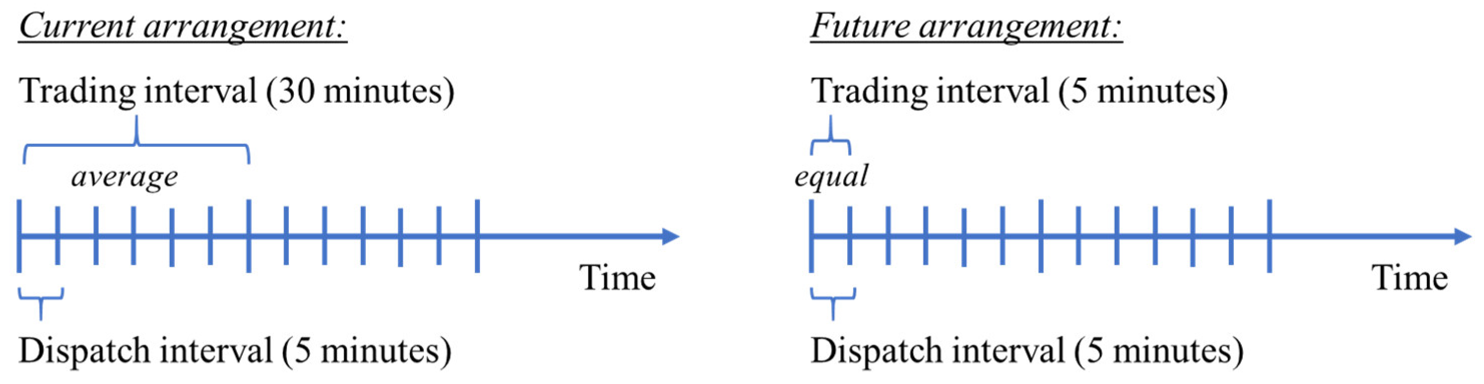
Figure 3.
FCAS raise contingency response (conceptual illustration). Adapted from [43].
Figure 3.
FCAS raise contingency response (conceptual illustration). Adapted from [43].
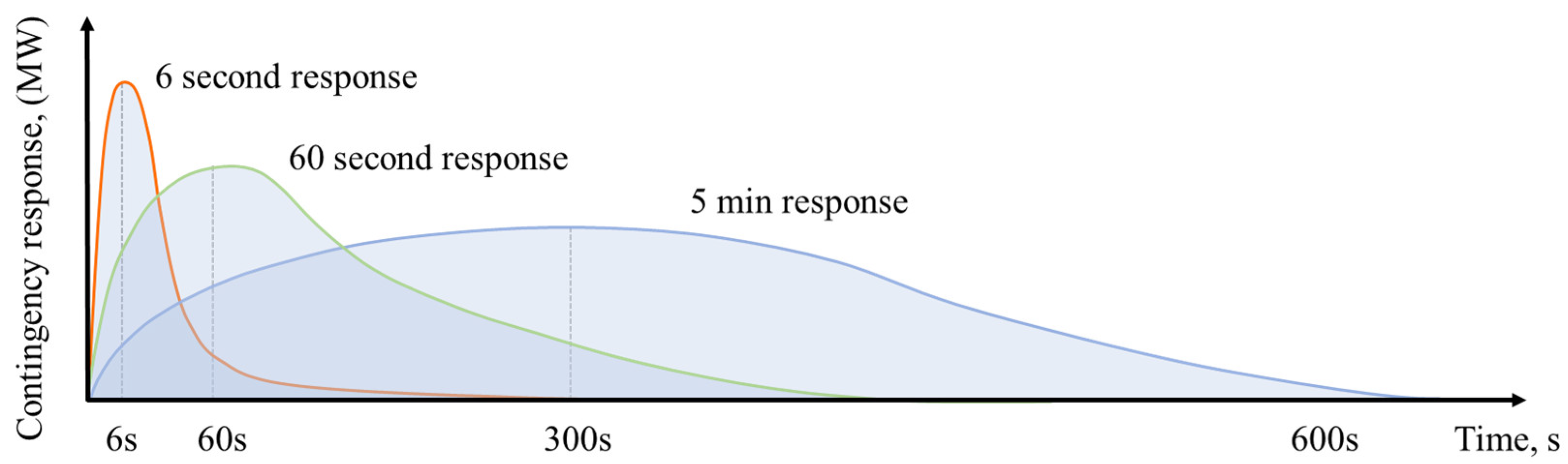
Figure 4.
Bi-directional operation of BESS, with example of combined energy and reserve bids in either generator or load operating mode.
Figure 4.
Bi-directional operation of BESS, with example of combined energy and reserve bids in either generator or load operating mode.

Figure 5.
Battery contingency FCAS response—10 December 2019 (Victoria and South Australia regional separation). Adapted from [44]-South Australia’s Virtual Power Plant.
Figure 5.
Battery contingency FCAS response—10 December 2019 (Victoria and South Australia regional separation). Adapted from [44]-South Australia’s Virtual Power Plant.
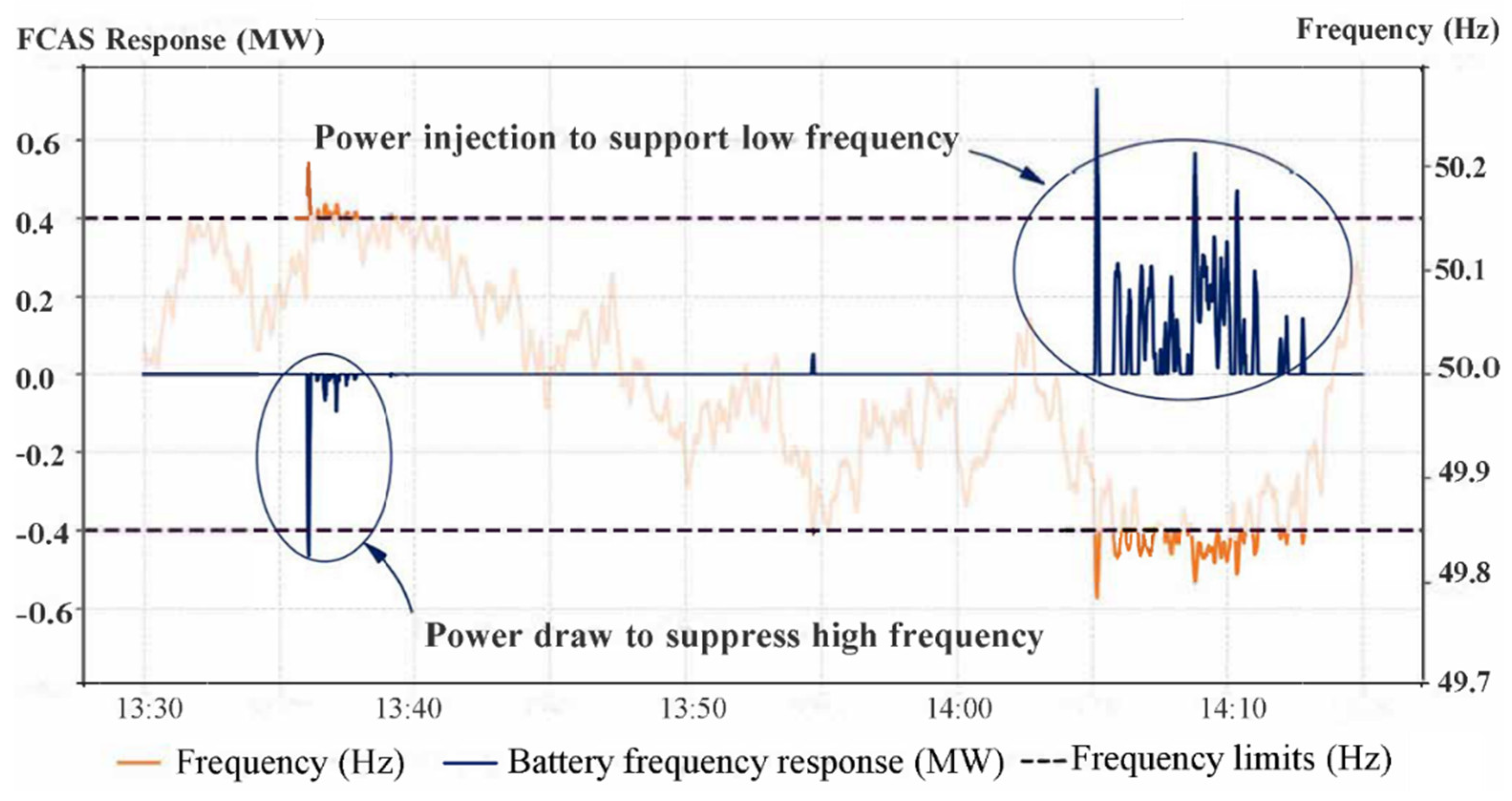
Figure 6.
Example of cycle counting using the rainflow algorithm.
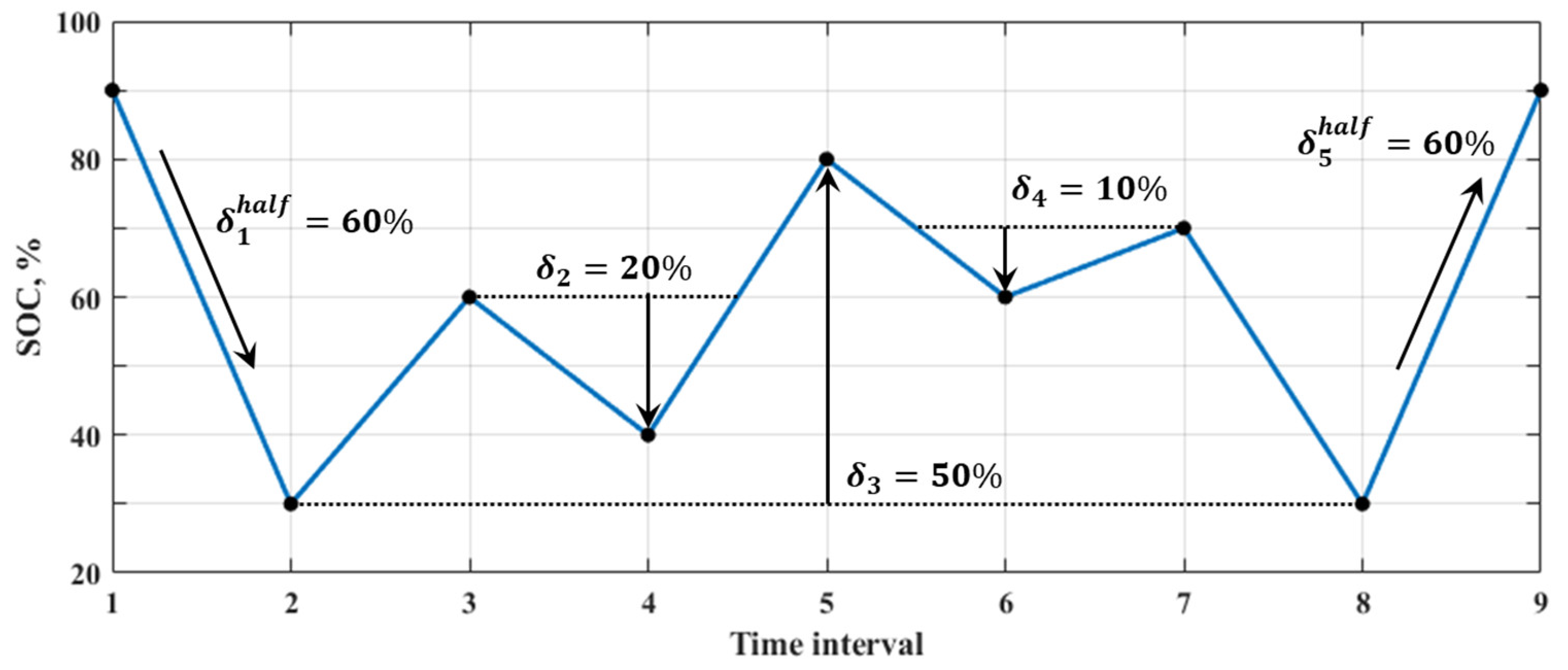
Figure 7.
Linearization of BESS degradation (for illustrative purposes).

Figure 8.
Example of energy spot price and 6 s raise contingency price over one day (NSW market).
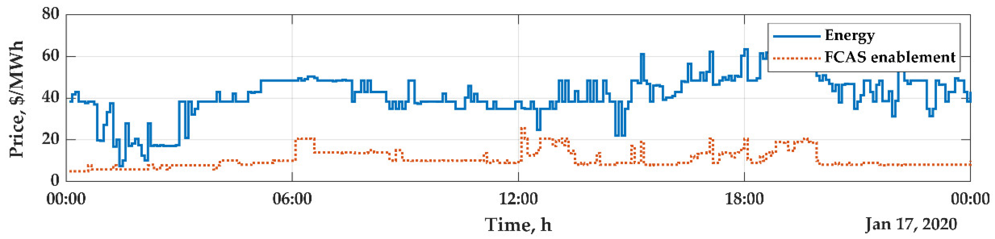
Figure 9.
Battery charge and discharge actions (top) and resulting SOC (bottom) under Strategy 1 (maximization of revenue from spot energy market) for a single day of operation with market prices.
Figure 9.
Battery charge and discharge actions (top) and resulting SOC (bottom) under Strategy 1 (maximization of revenue from spot energy market) for a single day of operation with market prices.
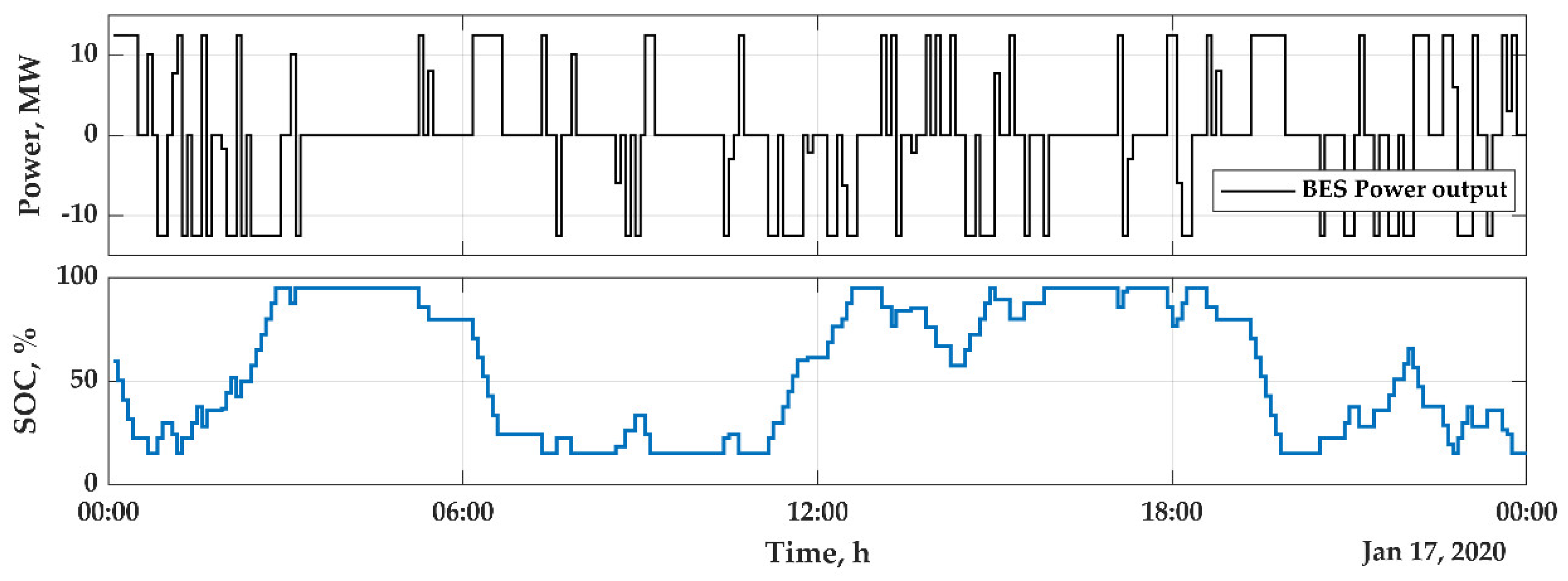
Figure 10.
Battery charge and discharge actions and FCAS enablement (top) and resulting SOC (bottom) under Strategy 2 (maximization of revenue from spot and FCAS markets) for a single day of operation with market prices.
Figure 10.
Battery charge and discharge actions and FCAS enablement (top) and resulting SOC (bottom) under Strategy 2 (maximization of revenue from spot and FCAS markets) for a single day of operation with market prices.
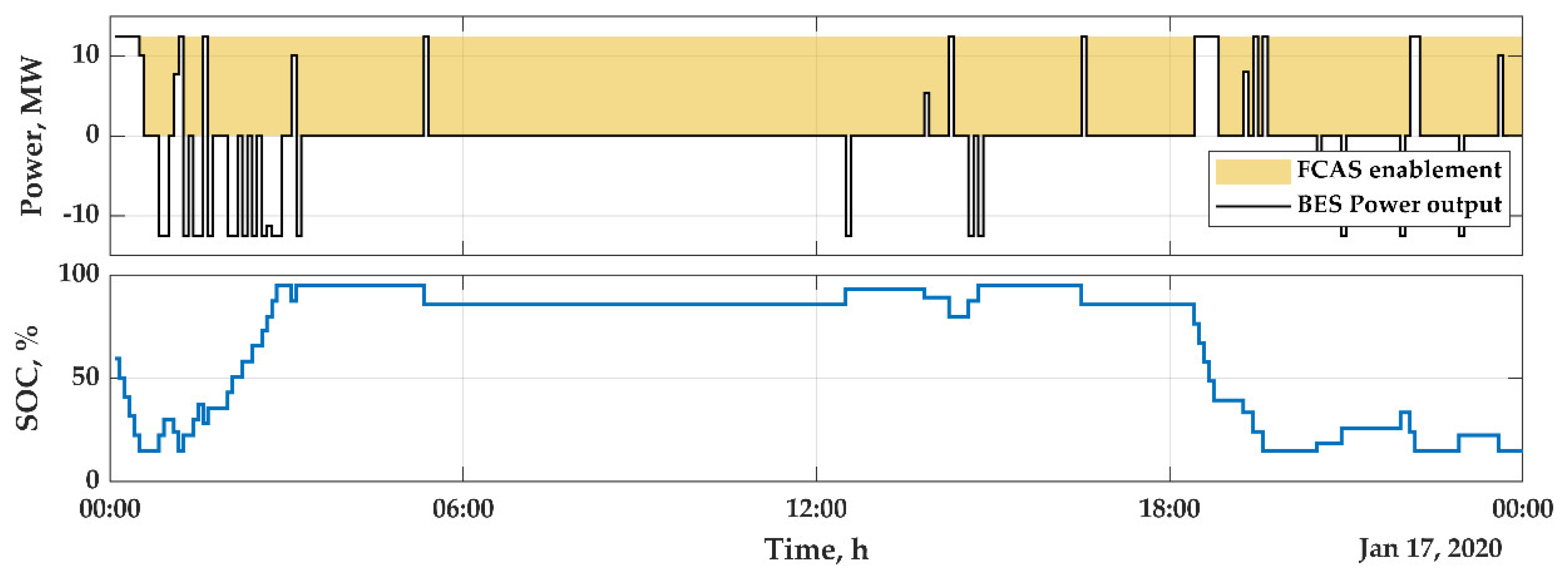
Figure 11.
Battery charge and discharge actions and FCAS enablement (top) and resulting SOC (bottom) under Strategy 3 (BESS operation based on the degradation cost function in spot and FCAS markets) for a single day of operation with market prices.
Figure 11.
Battery charge and discharge actions and FCAS enablement (top) and resulting SOC (bottom) under Strategy 3 (BESS operation based on the degradation cost function in spot and FCAS markets) for a single day of operation with market prices.
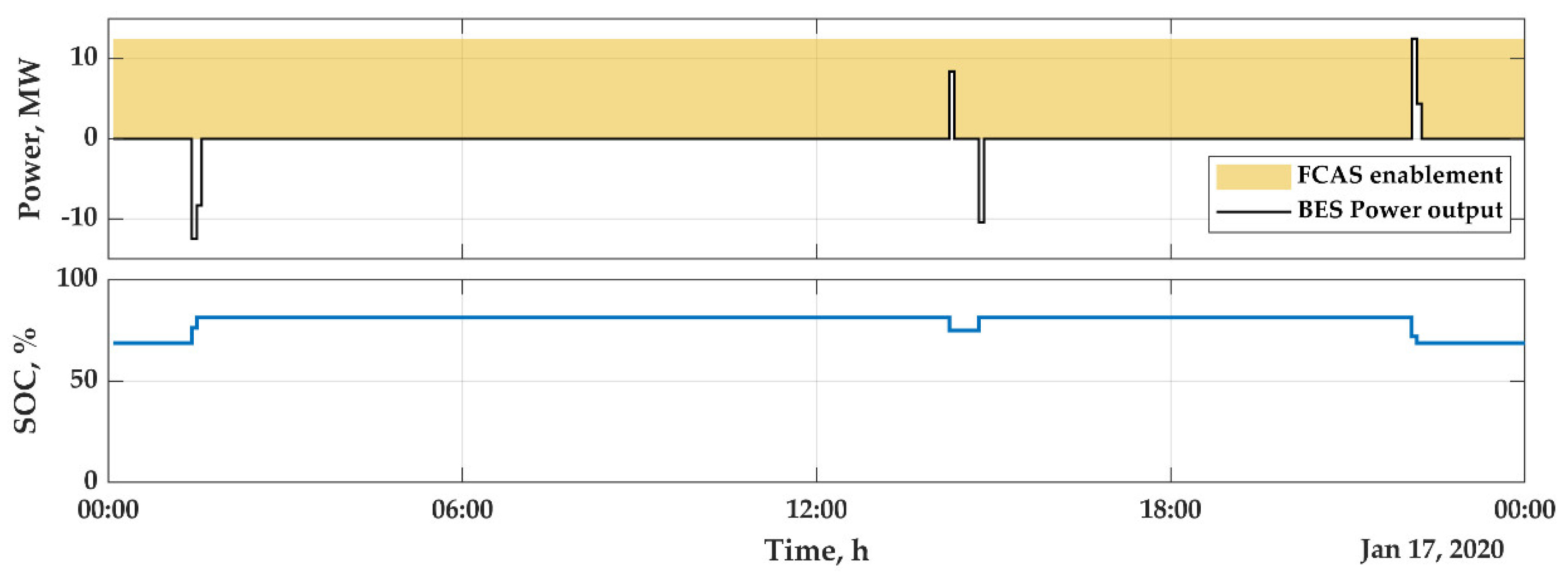
Figure 12.
Cost and revenue breakdown for each BESS strategy.

Figure 13.
Illustration of battery operation in energy and FCAS markets over a single day for NSW. Top plot: power outputs (positive values—discharging, negative—charging) and FCAS enablement (positive values—capacity reserved for raise FCAS markets, negative—for lower). Second plot: resulting battery SOC. Third plot: energy market price. Bottom plot: FCAS market prices.
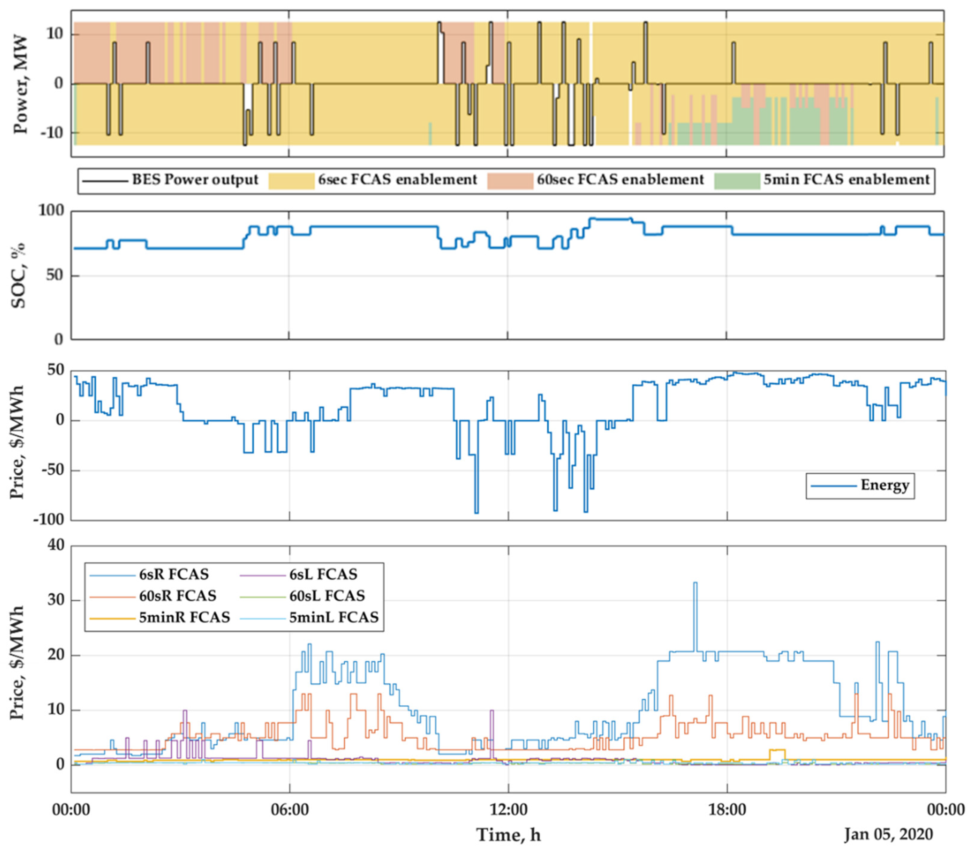
Figure 14.
One-year operation of the battery in regional markets of Australia.


Table 1.
Population, energy technology share and NEM spot price in 2020.
| Year 2020 | Tasmania | South Australia | Victoria | New South Wales | Queensland |
|---|---|---|---|---|---|
| Population (M) | 0.5 | 1.7 | 6.4 | 7.5 | 5.1 |
| Solar PV | 2% | 17% | 8% | 8% | 13% |
| Wind | 14% | 42% | 14% | 6% | 2% |
| Hydro | 83% | - | 5% | 3% | 1% |
| Gas | 1% | 42% | 3% | 2% | 11% |
| Coal | - | - | 74% | 73% | 80% |
| Imports | 12% | 7% | 3% | 8% | - |
| Exports | 12% | 8% | 7% | 0% | 7% |
| Renewables share | 99% | 59% | 27% | 18% | 16% |
| Price $/MWh | 43 | 43 | 61 | 68 | 43 |
Table 2.
FCAS markets in the Australian NEM.
| FCAS Type | FCAS Name | Function | General Description |
|---|---|---|---|
| Regulation | Raise | Correct minor drop in frequency | Designed to respond to small deviation in the frequency (up to ±0.15 Hz). The control is implemented using utomatic generator control (AGC). Units on regulation duties have to continuously adjust their operational set points, injecting more or less active power depending on control signals provided by AEMO. |
| Lower | Correct minor raise in frequency | ||
| Contingency | Fast raise | Provides an active power response within 6 s after frequency deviates away from normal operating band (NOB). It must be sustained for 60 s | Designed to respond to contingency events when frequency deviates away from normal operating band (NOB). No contingency response is provided if frequency stays within NOB (49.85–51.15 Hz) |
| Fast lower | |||
| Slow raise | Provides an active power response within 60 s after frequency deviates away from NOB. It must be sustained for 300 s | ||
| Slow lower | |||
| Delayed raise | Provides an active power response within 5 min after frequency deviates away from NOB. It must be sustained for 600 s | ||
| Delayed lower |
Table 3.
BESS specifications [47].
Table 3.
BESS specifications [47].
| Parameter | Value |
|---|---|
| Nominal capacity | 12.5 MWh/12.5MW |
| Charging/discharging power rating | 1C |
| Maximum SOC | 95% |
| Minimum SOC | 15% |
| Charging/discharging efficiency | 90% |
| Battery cycle life | 3000 cycles at 80% DOD 22,0000 cycles at 30% DOD |
| Battery shelf life () | 10 years |
| Cell temperature | Maintained at 25 °C |
| Battery-pack replacement cost | 380,000 AUD/MWh |
| Chemistry | Li(NiMnCo)O2 lithium-ion |
Table 4.
BESS bidding strategies.
| Strategy 1 | Strategy 2 | Strategy 3 | |
|---|---|---|---|
| Participation in the energy market | Y | Y | Y |
| Participation in FCAS market | N | Y | Y |
| Cycling degradation costs constraint | N | N | Y |
Table 5.
Outcomes from dispatch of 12.5 MWh BESS participating in Australian energy market (NSW, 2020).
Table 5.
Outcomes from dispatch of 12.5 MWh BESS participating in Australian energy market (NSW, 2020).
| Strategy 1 | Strategy 2 | Strategy 3 | |
|---|---|---|---|
| Revenue from the energy market | $1,585,793 | $1,450,624 | $1,217,395 |
| Revenue from FCAS market | $0.0 | $1,492,116 | $1,598,569 |
| Gross revenue | $1,585,793 | $2,942,740 | $2,815,964 |
| Battery cycling costs | $1,445,615 | $1,007,162 | $57,514 |
| Benefit after costs | $140,178 | $1,935,578 | $2,758,450 |
| Annual cycling degradation | 30.43% | 21.20% | 1.21% |
| Equivalent cycles (@80%DOD) | 913.6 | 636.5 | 36.3 |
| Battery life expectancy (years) | 3.29 | 4.72 | 10.00 |
Publisher’s Note: MDPI stays neutral with regard to jurisdictional claims in published maps and institutional affiliations. |
© 2021 by the authors. Licensee MDPI, Basel, Switzerland. This article is an open access article distributed under the terms and conditions of the Creative Commons Attribution (CC BY) license (https://creativecommons.org/licenses/by/4.0/).
Share and Cite
MDPI and ACS Style
Bayborodina, E.; Negnevitsky, M.; Franklin, E.; Washusen, A. Grid-Scale Battery Energy Storage Operation in Australian Electricity Spot and Contingency Reserve Markets. Energies 2021, 14, 8069. https://doi.org/10.3390/en14238069
AMA Style
Bayborodina E, Negnevitsky M, Franklin E, Washusen A. Grid-Scale Battery Energy Storage Operation in Australian Electricity Spot and Contingency Reserve Markets. Energies. 2021; 14(23):8069. https://doi.org/10.3390/en14238069
Chicago/Turabian StyleBayborodina, Ekaterina, Michael Negnevitsky, Evan Franklin, and Alison Washusen. 2021. "Grid-Scale Battery Energy Storage Operation in Australian Electricity Spot and Contingency Reserve Markets" Energies 14, no. 23: 8069. https://doi.org/10.3390/en14238069
Note that from the first issue of 2016, this journal uses article numbers instead of page numbers. See further details here.