
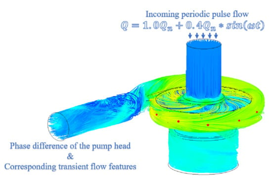
Flow Stability in a Miniature Centrifugal Pump under the Periodic Pulse Flow

1
Faculty of Mechanical Engineering and Automation, Zhejiang Sci-Tech University, Hangzhou 310018, China
2
School of Energy and Power Engineering, Xi’an Jiaotong University, Xi’an 710049, China
*
Authors to whom correspondence should be addressed.
Energies 2021, 14(24), 8338; https://doi.org/10.3390/en14248338
Submission received: 20 October 2021
/
Revised: 5 December 2021
/
Accepted: 6 December 2021
/
Published: 10 December 2021
(This article belongs to the Topic Energy Storage and Conversion Systems)
Abstract
:The flow behavior inside a miniature centrifugal pump, under a periodic pulse flow rate, was studied by means of numerical simulation. For a given incoming periodic pulse flow with a sine wave, the performance of the centrifugal pump was investigated in the section with increasing flow and the section with decreasing flow, and the special points of the flow rate and the periodic flow were identified. Further, the energy gradient method and the Q-criterion were adopted to analyze the internal vertical structure and flow stability. It was found that the regions with large variations in velocity and total pressure were mainly located at the leading edge of the suction surface and the middle area of the pressure surface of the blades. Irregular pressure fluctuation frequency under the periodic pulse flow was shown; this was mainly concentrated in the low-frequency zones close to the impeller’s rotational frequency. In addition, for the same flow rate in the periodic pulse flow, the pressure frequency fluctuation for the increasing flow rate section was higher than that observed for the decreasing flow rate section. It was found that the most unstable sections appeared in the first half-period of the flow rate variation (large flow rate), according to the distributions of the Q criteria of the vortex and the energy gradient function K. In this section, motions of strong vortices led to large gradients of the mechanical energy.
1. Introduction
The miniature centrifugal pump has a characteristic dimension of 1–50 mm. It has promising application prospects, especially for micro transport system devices. The special geometric dimension, suspended impeller as well as the hydraulic features have caused extensive concerns in fluid mechanics. Since the external performance of the pump system is determined by internal flow, the unstable flow phenomenon is the main reason for energy loss and hydrodynamic noise [1]. To enhance the performance of the miniature pump, further investigation on the internal flow and hydraulic performance are needed. In particular, periodic pulse flow is one of the main features of miniature centrifugal pumps used for heart medical applications.
Essentially different from the fixed constant flow rate, periodic variable flow is the process of continuous flow change, which reflects some peculiar features. Taylor et al. [2] pointed out that creating accurate physiological circulatory conditions is beneficial to the evaluation of cardiac assist technologies. Salewski et al. [3] and Stanfield et al. [4] investigated the minimal-access left ventricular assist device (LVAD) implantation, and stressed its importance for microfluidic transport under periodic pulse flow. Salama [5] numerically investigated the flow reversal phenomenon caused by the change of the pump flow rate, and discussed the corresponding thermal–hydraulic transients in the fast loss of flow accident (FLOFA).
Research has been carried out on the hydraulic performance of miniature pumps. Wu et al. [6] investigated the pressure gradient and multiple vortices in a miniature magnetically levitated centrifugal pump. Paul et al. [7] investigated the hydraulic performance of a shrouded centrifugal impeller with different passage curvatures and tip clearances. Taskin et al. [8] studied the distribution of pressure and shear stress in a wearable artificial pump lung. To investigate the pulsatile flow features caused by the heart pumping process, works on pulsatile flow have been carried out. Lee et al. [9] proposed that the pumping process of the heart can be regarded as the course with sinusoidal changes. Zhuang et al. [10] conducted a study on a double-suction miniature pump, and it was suggested that the flow function during heart pumping can be considered as a superposition of several sinusoidal functions. Furthermore, Nosé et al. [11] researched the cardiac pumping effect on the flow of the bloodstream by studying the simplified pressure or flow rate output. Lee et al. [12] pointed out that the miniature pump under periodic variable flow presents a different hydraulic performance.
Qian et al. [13], Xin et al. [14], and Bumrungpetch et al. [15] conducted a series of works to obtain a pulsating pump with low hemolytic blood flow and a better flow stability in blood pump. They stressed that it is important to study the pulsatile flow in terms of differences in hydraulic performance between the pulsatile and non-pulsatile ventricular assisting devices.
Li et al. [16] studied the flow instability in a miniature centrifugal pump at a constant flow rate based on the energy gradient method. The unstable zones in the impeller were identified using energy gradient analysis. However, the blood pump often works at a periodic flow rate, which results in peculiar features and hydraulic performance vibration. The pump requires better flow stability in the pumping process to provide a comfortable environment to customers. Therefore, it is important to study the influence of periodic flow rate on flow stability in the pump in order to improve the stability of flow and to enhance the working quality of the pump.
In present study, the internal flow parameters in the impeller of a miniature centrifugal pump under the periodic inlet pulse flow were studied. Numerical simulation of the internal flow of the miniature pump was performed with Navier–Stokes equations. The flow stability was analyzed with the energy gradient method. The hydraulic performance, the differential analysis, energy field analysis and the spectrum analysis of pressure pulsation were adopted to characterize the peculiar internal flow performance. The differences in the constant incoming flow and periodic inlet pulsation flow were observed, and the influence of the periodic inlet flow on the stability was clarified.
2. Numerical Methods and Modeling
2.1. Parameters of the Miniature Centrifugal Pump
The miniature pump analyzed in present paper was used as a blood pump. Figure 1 visualizes the geometry of the miniature centrifugal pump. The computational domain consists of seven parts: the inlet, volute, impeller with five backward curved blades, two side chambers, and the extended inlet/outlet duct. The miniature centrifugal pump under investigation has a characteristic dimension of 33 mm. The impeller is magnetically levitated and five backward blades rotate at the operating rotating speed at 8000 rpm. The inlet diameter is 10 mm, and the narrow gap between the impeller and back chamber is 0.5 mm. The design flow rate of the pump is 0.48 m3/h. Table 1 presents a summary of the main parameters of the pump.
2.2. Function of Periodic Pulse Flow and Its Section Division
The typical sine wave function was selected to simplify the pump processing. Based on the actual design and operating conditions of this model pump, the function of the sinusoidal flow rate was changed as follows: the initial value of the flow function was set as the design flow rate 1.0Qn. To avoid extreme flow rates, the range of fluctuation of this flow function was set as ±0.4Qn. The function of the inlet sinusoidal flow can be expressed as:
where Q denotes the flow rate of the periodic inlet pulse flow, Qn is the design flow rate and t denotes the operating time. In Equation (1),
where T indicates the time consumed by one impeller cycle. The selected sinusoidal flow function has the variation period of 0.27 s, which means that one sine wave period includes 36 cycles of pump rotation.
The internal flow of the miniature centrifugal pump under the four sinusoidal flow period was calculated, and the internal flow parameters during the third sine period were selected for the specific analysis. Figure 2 shows the case points selected for study during the third sine cycle of the incoming periodic pulse flow, which will be detailed in the following sections.
Table 2 shows the three different flow sections and their corresponding cases for the third sine period. Based on the cyclical variation of the flow rate and in order to facilitate the unification of symbols, the next case of case 12 is still marked as case 1, and so on. It is notable that the cases 1 and case 7 are located at different flow conditions although they have the same flow rate.
2.3. Governing Equations and Mesh Generation
The governing equations can be expressed by the time-dependent three-dimensional incompressible Reynolds-averaged Navier–Stokes equations, which can be described as:
where, u, v, and w denote the velocity component in the x, y, and z directions, t is the time, p is the pressure, and Su, Sv, and Sw denote the generalized source terms, respectively.
The finite volume method (FVM) was employed to solve the system of equations with the ANSYS-CFX (Canonsburg, PA, USA). The SST k-ω turbulence model was employed to couple governing equations, similar to Li et al. [16] and Wu et al. [17]. Numerical investigation of the hydraulic performance of the miniature centrifugal pump was conducted on the working station with 48 cores (Intel Xeon at 3.0 GHz, INSPUR Co., Ltd., Jinan, China). Furthermore, the inlet boundary was located three average impeller diameters upstream of the impeller’s inlet, and the static pressure outlet boundary was located three average impeller diameters downstream of the volute outlet. The turbulence intensity at the inlet boundary was 5%. The total pressure was given as 101.325 Pa and was normal to the outlet boundary.
As illustrated in Figure 3, the structured mesh was adopted in the inlet, front chamber, impeller and back chamber, and the refined unstructured mesh was generated in the eccentric volute. The mesh generated for the narrow gaps was refined, such as the clearance in the front chamber and the clearance between the impeller and the back chamber. Meanwhile, the wall mesh Y plus for the overall model was 0–45, and was 0–20 for the impeller domain. The selection of Y plus was in good agreement with the requirements of the SST k-ω turbulent model.
The non-dimensional head coefficient ψ is defined as,
where r is the outer radius of the impeller.
The power coefficient Pc can be expressed as,
where ρ is the fluid density and M denotes the measured torque.
Variations of the calculated head coefficient ψ and power coefficient Pc for the four sets of meshes are given in Table 3. It was found that mesh independence could be confirmed. With the mesh number increasing, the relative change of the head coefficient (ψ) was −1.46% for 4.31 million, −0.59% for 6.68 million and −0.30% for 10.8 million. Meanwhile, the relative change of the power coefficient (Pc) was −3.12% for 4.31 million, −2.59% for 6.68 million and −0.16% for 10.8 million. The relative changes in ψ and Pc were not very significant with the increasing of the mesh number when the mesh number was more than 6.68 million cells. Finally, the case with 6.68 million cells was chosen for the following simulations.
3. Briefs of Energy Gradient Method
Recently, Dou and co-authors [18,19,20] proposed the energy gradient method to analyze the flow instability and turbulent transition. The energy gradient function, which represents a local Reynolds number, is employed to characterize the local behavior of flow stability. The maximum of the energy gradient function represents the most unstable position in the flow field. The method has been successfully applied to analyze the flow stability in rotating devices [21] and centrifugal pumps [16] as well as centrifugal compressors [22].
According to the energy gradient method, the energy gradient function K indicates the ratio of the amplification of disturbance energy and the damping of disturbance due to viscous friction. Regions with large magnitudes of K are more unstable than those with low magnitudes of K, and the position with the maximum Kmax is the most dangerous position in terms of initiating instability. For a given flow, Dou [15,16,17,18,19] proposed that the K can be expressed as follows for shear-driven flows,
Here, K is a dimensionless field function, s denotes the transverse direction, and n is measured along the normal direction. V denotes the total velocity, E is the total mechanical energy per unit volume, and W is the work conducted by shear stress along the streamline for a finite length.
The total mechanical energy gradient along the direction normal to the streamline can be written as
where P denotes the static pressure.
In shear-driven flows, the rate of work conducted by the tensor of shear stress on the unit volume of fluid can be expressed as follows for steady flows,
In these equations, φ is the rate of energy dissipation and can be written as
where D is the strain rate tensor and μ is the dynamic viscosity. These equations were used to calculate the vortex breakdown in a rotating cylinder with the bottom rotating, and good agreement was achieved with experimental data.
The calculation of the energy gradient function K and the related quantities were completed using in-house code for the given flow field.
4. Results and Discussion
4.1. Pump Head under Incoming Constant Mass Flow and Incoming Periodic Pulsating Flow
The hydraulic performance of the miniature centrifugal pump at the constant incoming flow is presented in Figure 4. With the increase in the flow rate, the head increased in the low flow rate regime, and decreased in the high flow rate regime. The pump head, at a constant incoming flow, showed a hump-like distribution, which indicated that the pump was prone to inducing flow instability under the off-design load. The head under the fixed constant flow rate varied in the range of 11.73–12.02 m.
Figure 5 shows the variation of the head of the pump with the time for the second and the third cycle of periodic incoming pulsation flow. The head under this rate of periodic inlet pulse flow had a fluctuation range of 11.38–12.03 m. Under the influence of the sinusoidal flow rate, the head of miniature pump presented a sinusoidal distribution, although there was a slight fluctuation.
Combining Figure 4 with Figure 5, the maximum head under both a variable flow rate and a fixed flow rate was around 12.00 m, while the miniature head presented a significant difference. The pump head, under the incoming flow of the periodic inlet pulsation, was much lower than that of the constant incoming flow at the flow rate Q/Qn = 0.6 or Q/Qn = 1.4. This indicates that there existed a more complex internal flow performance and a strong flow variation for the periodic pulse flow.
Figure 6 shows the sinusoidal-like distribution of the head under the periodic incoming pulsation flow and the given periodic flow rate, respectively. It is seen that there was a certain phase difference between the flow’s sinusoidal waveform distribution and the head’s sinusoidal waveform distribution. Case 10 (corresponding t = 0.6075 s, Q = 0.6Qn), which exhibited the minimum flow rate, and case 4 (corresponding t = 0.7425 s, Q = 1.4Qn), which also exhibited the maximum flow rate, did not reach the maximum/minimum values for the head. For the same flow rate Q = 1.0Qn, the head under the fixed continuous flow rate was 11.93 m, while it was 11.78 m for case 1 and 12.00 m for case 7, and case 7 had the highest head. It is noticed that case 1 was located in the increasing flow rate section, and case 7 was located in the decreasing flow rate section. The phase difference between the head and flow rate was mainly caused by the hysteresis effect of the periodic inlet pulse flow.
4.2. Internal Flow Parameters in the Increasing Flow Rate Section
The velocity and total pressure for case 1 under the design flow rate was selected as the base data for the differential analysis. The variation between case 11 and 12 was the result of subtracting cases 11 and 12 from case 1. Additionally, cases 2 and 3 were the result of the subtraction of case 1 from case 2 and 3. Cases 11, 12, 2 and 3 were the cases in the increasing flow rate section.
Large variation values indicated huge changes in velocity/total pressure. In Figure 7a,b, the velocity variations for cases 11 and 12 show a similar distribution. Fields with high velocity increases were mainly located at the leading edge and the trailing edge of the suction surface, and also at the leading edge and the middle region of the pressure surface. It is important to note that the velocity was observed to change more rapidly in the areas near the pressure surface.
In Figure 7c,d, the velocity variation for case 2 and 3 reached the maximum in the “swirling” region, marked in Figure 7d near the leading edge. During the increasing of the flow rate from case 1 to case 3, there was still a large velocity variation in the leading edge of the suction surface. In addition, the region with large positive velocity variation was located in the middle suction surface and extended out to the pressure surface’s trailing edge.
The differential analysis of the total pressure on the center plane for cases 11, 12, 2 and 3 was carried out. In Figure 8a,b, with the increasing of the flow rate from a low flow rate to the design flow rate, the distribution of the total pressure variation shows an overall increasing tendency. The main areas of increase were concentrated around the leading edge of the suction surface and the trailing edge of the pressure surface. With the increasing of the flow rate, the region with increasing total pressure and the region with decreasing total pressure were mainly located around the leading edge of the suction surface. This was mainly affected by the small separating vortices generated at the blade’s leading edge.
Figure 8c,d shows the total pressure variation from the design flow rate to the high flow rate. During this process, the areas of increasing total pressure were mainly concentrated in the impeller passage and regions near the pressure surface. Conversely, in case 11 and 12, for the regions near the leading edge of the suction surface, the areas of increasing total pressure transferred to the areas where pressure was reduced. Both the fields with increasing total pressure and the fields with decreasing total pressure existed simultaneously in the vicinity of the leading edge of the suction surface. This phenomenon at the leading edge was mainly caused by the effect of the small-scale separation vortices.
In Figure 9a,b, regions with strong vortex intensity were mainly located in the leading edge and the middle area of the suction surface. For the miniature centrifugal pump, there was a narrow space between the impeller and the back chamber. As a result of the rotor–stator interaction between the high speed impeller and the static back case, as shown in Figure 9a,b, the flow field inside this narrow space had high vortex intensity. It is worth nothing that the regions with separation vortices near the leading edge of the suction surface showed good agreement with the regions with high variations of velocity and total pressure, as shown in Figure 7 and Figure 8. This indicated that the separating vortices had a huge effect on the local velocity and total pressure.
In Figure 9c, in the middle area near the suction surface, one vortex core shifted into two vortex cores. This indicates that with the flow rate entering into the large flow regions, the shedding of the small-scale vortices on the suction surface became more frequent. This further led to the increasing of the number of small-scale vortices in the impeller passage. Furthermore, as a result of the geometry curvature of the impeller’s inlet, “circular ring” regions with strong vortex intensities appeared near the impeller’s inlet. The emerging “circular ring” regions could be explained in terms of the strong collision impact between the fluid particles and the impeller’s solid wall.
According to the energy gradient theory, the velocity gradient and the pressure gradient are one of the most important parameters. In Figure 10, it can be seen that with the increasing of the flow rate, the regions with the high values for the energy gradient function K under the periodic inlet flow presented an expanding trend. Large values were observed for the energy gradient function K in the areas where the velocity/total pressure had drastically changed, which further characterized those areas that had high K.
As shown in Figure 10, the regions with Kmax were located along the middle and the trailing edge of the pressure surface and the impeller exit near the trailing edge of the pressure surface. In Figure 10, the “circular ring” it can be seen that regions near the impeller entrance also presented high mechanical energy gradients. This was the result of the sudden change of velocity direction at the impeller’s inlet as well as the strong collision impact between the fluid particles and the impeller’s solid wall.
4.3. Internal Flow Parameters in the Decreasing Flow Rate Section
In this section, the velocity and total pressure for case 7 under the design flow rate are selected as the data to be used in the differential analysis. Cases 5, 6, 8 and 9 are the cases in the decreasing flow rate section.
As presented in Figure 11, during the process in which the flow rate decreased from a large flow rate to the designed flow rate, the main regions on the center plane showed a decreasing velocity. Fields with the increased velocity were mainly located in the areas of the leading edge of the suction surface, the middle position of the pressure surface and the exit of the impeller. In Figure 11a, two regions can be identified with large velocity variation around the suction surface’s leading edge. This was mainly because the shedding vortices influenced the local velocity field and the pressure field, which further intensified the velocity change. Figure 11c,d shows that with the flow rate decreasing from the design flow rate to a low flow rate, the distribution of the positive velocity variation was different from that of case 11 and case 12 in Figure 7. This indicates that at the same flow rate, different tendencies in the variation of the flow rate led to different degrees of velocity variation.
The results of the differential analysis of the total pressure on the center plane for cases 5, 6, 8 and 9 are shown in Figure 12. The total pressure variation for case 5 and case 6 was mainly negative, and the decreasing areas were located in the leading edge and the trailing edge of the pressure surface. In the leading edge of the suction surface, both the fields with increasing total pressure and the fields with decreasing total pressure existed simultaneously. With the flow rate decreasing from a high flow rate to the design flow rate, the areas with increased total pressure, for case 5 and case 6, were mainly concentrated around the leading edge and the trailing edge of the pressure surface. With the decreasing of the flow rate from the design flow rate to the low flow rate, the total pressure, for case 8 and case 9, exhibited an increasing trend. Furthermore, the regions with increased total pressure were located at the leading edge and the trailing edge of the pressure surface.
Regions with strong vortex intensity in the impeller for the decreasing flow rate section are shown in Figure 13. Fields with strong vortex intensity were mainly located in the leading edge, the middle area of the suction surface as well as the narrow clearance between the impeller and the back chamber. In the leading edge and middle area of the suction surface, there were regions with different vortex intensities and different vortex scales, that is, the flow structures in these areas were dominated by strong vortex intensity.
In the decreasing flow rate section, the vortex intensity of internal flow was more complicated than that of the increasing flow rate section. In Figure 13a,b, it can be seen that there was stronger vortex intensity for the shedding vortices near the leading edge of the suction surface.
Figure 14 shows the distribution of the energy gradient function K in impeller for the decreasing flow rate section. In Figure 14a,b, it is shown that fields with the Kmax were mainly located in the middle area and trailing edge of the pressure surface. With the decreasing of the flow rate, regions with Kmax inside the impeller showed a gradually decreasing trend. It is worth noting that, considering the above in combination with Figure 1c,d, it can be seen that the vortices in the impeller passage affected the local velocity field and the total pressure field, which further influenced the local mechanical energy field and local shear strength. Furthermore, the changed mechanical energy and shear strength were then captured by the energy gradient function K. In addition, the “circular ring” regions near the impeller’s inlet with Kmax decreased gradually as the flow rate decreased.
4.4. Internal Flow Parameters for Special Positions of the Flow Function
After the differential analysis of the flow characteristics of the increasing flow rate section and the decreasing flow rate section, the flow characteristics of the special position of the periodic variable flow function were further observed and analyzed.
In this section, the two extremum positions of the flow function and the two design flow rates (the same flow rates with the different flow rate trends) were investigated, respectively. The corresponding relationship among the four cases was: case 1 was the design flow rate with a positive slope of the flow function, case 4 was the maximum point of the flow function, case 7 was the design flow rate with a negative slope of the flow function and case 10 was the minimum for the flow function.
In Figure 15a,c, it is shown that the fields with strong vortex intensities presented a similar distribution for both case 1 and case 7 under the design flow rate. Both of them had two vortex cores in their separation vortices at the leading edge of the suction surface. However, in the middle area of the suction surface, the vortex intensity for case 1 was lower than that of case 7. The contour diagram for case 1 shows the single vortex core distribution, and the contour diagram for case 7 shows two vortex cores in the same region. In Figure 15, the vortex core distribution inside the impeller for case 4 is shown to be more extensive than those of the other three operating conditions.
The distribution of the fields with strong vortex intensities were different for the fixed constant flow rate and the periodic inlet pulsation flow. For the same flow rate of 1.0Qn, fields with strong vortex intensities were mainly located in the outer layer of the large-scale vortices under the fixed constant flow rate, as well as the leading edge and middle area of the suction surface.
To further study the peculiar features under this rate of periodic pulsation flow of the inlet, time-domain analysis and frequency-domain analysis were carried out. The pressures measured from the monitoring points around the impeller in the four different cases are shown in Figure 16. The monitors are numbered clockwise, and the monitor that is located near the impeller tongue is named monitor 1.
In addition, pressure pulsation at monitors near to/far from the pump tongue presented similar time-domain and frequency-domain characteristics. Therefore, the following investigation on the pressure pulsation is divided into two parts: the near tongue monitors (monitor 1, monitor 2, monitor 3 and monitor 8) and the far tongue monitors (monitor 4, monitor 5, monitor 6 and monitor 7).
In the following investigation, the pressure pulsation for both the constant incoming flow and periodic incoming pulsation flow is carefully studied and compared. Considering that the incoming periodic pulsation flow was constantly changing with time, the time-domain and frequency-domain analysis of the pressure were conducted based on the monitor data of ±0.5 rotation cycles around the analyzed cases. For cycles with variable flow regimes containing 36 centrifugal pump cycles, the pressure changes in the selected ±0.5 rotation cycles were negligible.
The impeller diameter D1 of this pump was 33 mm, and the circumference diameter of each monitoring point was 35 mm. As shown in Figure 16, eight monitors were evenly distributed in the circumferential direction. The miniature centrifugal pump had a design speed of 8000× g rpm, the impeller’s rotational frequency F = 133.33 Hz, and the blade-passing frequency Fb = 5F ≈ 666.6 Hz.
A periodicity characteristic of the time-domain pressure was observed, and is presented Figure 17. The pressure value at monitor 2 was the smallest, but it showed the largest change in pressure amplitude among all the detection points. Monitor 2 was located in the area near the pump outlet and the impeller tongue, where unstable structures such as the “jet-wake” structure and the separation vortex could not be neglected. These unstable structures aggravated the complexity of local flows and were reflected in the range of pressure amplitude variation at monitor 2. Similarly, the circumferential position of the monitor points 4, 5, 6 and 7 were far away from the tongue, which resulted in the corresponding pressure amplitude variation range being small and the overall regularity being relatively uniform.
Under the different incoming flow rates, the main frequency of the pressure pulsation was always located at the blade-passing frequency Fb and the multiple blade-passing frequency m × Fb (m = 1, 2, 3…), and the amplitude of the other frequency division was much lower. For the same monitor (the impeller’s circumferential position), the pressure frequency at the 0.6Qn flow rate was higher than that in the design condition 1.0Qn and the large flow condition 1.4Qn, and the main pressure frequency tended to decrease with the increasing of the flow rate. This might have been due to the fact that the flow structure in the impeller was more complex under the small flow rate, and the larger dominant frequency peak may have been related to the collision of the multi-scale vortex structures.
Furthermore, monitor 1 and monitor 2 were located near the tongue, and their dominant frequency amplitudes at 0.6Qn were much higher than those at other monitors, which further verified that the internal flow conditions near the tongue were poor and that there was a huge pressure instability. With the increasing of the flow rate, the amplitude of pressure frequency at monitor 1 and 2 decreased significantly.
Figure 18 visualizes the transient Energy gradient function K (define Kmax = 30) performance in the pump impeller. Compared with the vortex core distribution (visualized by QT), it can be seen that the distribution of the energy gradient function K in space had a certain overlap with the vortex core distribution, especially in the outer layer of the large-scale vortices. In addition, the flow instability, which was affected by the wake-jet regions, was also reflected by the K function.
At the times of T, T + 9 × ∆t and T + 18 × ∆t, the regions with Kmax agreed fairly well with the jet-wake structure and the large-scale vortices near the impeller tongue, which implied that the local flow instability was caused by the strong jet-wake structure and the influence of the impeller. When the time increased, the relative location of the impeller and impeller tongue was changed, which led to a strong interaction occurring in the local field. The corresponding changes in the separation passage vortices and the local flow instability were also reflected by the energy gradient function K.
The variation of the impeller pressure under periodic pulse flow was very different from that observed at a fixed constant flow rate. The different manifestations were as follows: the time-domain analysis of the pressure pulsation under the fixed flow rate was highly periodic, while that under periodic pulse flow was not. There was also a great difference between the pressure fluctuation spectrum range and the pressure fluctuation period. The large difference in pressure pulsation indicated that the flow characteristics under periodic pulse flow had their own features, and could not be fitted with the fixed constant flow rate cases.
Figure 19 shows the time-domain and frequency-domain analysis of pressure pulsation spectrum for case 1 and case 7. The two cases had the same flow rate and different flow rate trends. The monitors 1, 2, 3 and 8 near the tongue were selected to study the circumferential pressure performance.
Figure 19 shows that, for the same monitoring points, the pressure fluctuation spectrum amplitudes for case 1 and case 7 were different. In the frequency-domain analysis of pressure pulsation, the main pressure fluctuation frequency of case 1 was smaller than Fb ≈ 666.6 Hz, and was close to the impeller’s rotational frequency F = 133.33 Hz. The frequency-domain for case 1 remained in the low-frequency composition category, and the overall frequency composition was mainly concentrated at a level that was twice that of the blade-passing frequency. The main pressure fluctuation frequency of case 7 was close to its impeller’s rotational frequency F = 133.33 Hz; the fractional frequency of the pressure was mainly concentrated at a level that was one to two times the impeller’s rotational frequency, denoted as F. Compared with case 7, the amplitude of the dominant pressure frequency for case 1 was much larger. The generation, separation and fragmentation of vortices and the collision between flow particles were the source of low-frequency pressure pulsation. The case with the complex low-frequency pressure pulsation indicated that the internal flow was highly complex and unstable. Case 1 and case 7 showed different distributions in terms of the fractional frequency of the pressure. This indicated that the flow instability in the impeller was more likely to occur in the cases under the rising section than those under the decreasing section.
In Figure 20, case 4 is the case with the maximum flow rate, and case 10 is the case with the minimum flow rate. The pressure fluctuation spectrum for case 4 was mainly located within one or two times the blade-passing frequency Fb. Furthermore, there were some fractional frequencies of pressure that exceeded two times the blade-passing frequency Fb for case 10. For the same monitoring point, the pressure amplitude for case 4 was also lower than that for case 10.
It is seen from Figure 20 that the main pressure fluctuation frequency for case 4 was equal to the blade-passing frequency Fb. Comparing the pressure spectrum for case 4 with that of 1.4Qn under a fixed constant flow rate, the amplitude of main pressure fluctuation frequency under periodic pulse flow showed a smaller amplitude than that obtained under a fixed constant flow rate. Subjected to the effect of periodic pulse flow, many low-frequency components for case 4 were less than twice the blade-passing frequency (2Fb), and they were mainly located around the impeller’s rotational frequency F (133.33 Hz).
In addition, different from case 4, with the minimum flow rate, the main pressure fluctuation frequency for case 10 was around the impeller’s rotational frequency F = 133.33 Hz and the pressure amplitude was much higher than that for case 4. The components’ pressure pulsation spectra were concentrated at a level of two times the blade-passing frequency Fb.
The far more complex and lower amplitude of the fractional frequency of the pressure further illustrated the complex internal flow structures around the impeller at low flow rates. In the impeller, the unstable flow structures included the “jet-wake” structure and various scales of the separation vortices. The collisions and static pressure exchange between these unstable flow structures led to the local pressure and local pressure pulsation spectrum reaching its low flow value for case 10.
Finally, based on the energy gradient method, the distribution of the energy gradient function K of the four cases with special flow rates were analyzed. The parameters of the flow inside the impeller were captured and investigated from the perspective of the energy field. In general, the distributions of the flow fields with large K values were roughly the same for the four cases. As shown in Figure 21, the regions with the Kmax were mainly located in the middle and the trailing edge of the pressure surface, the exit of the impeller passage and the “circular ring” regions near the impeller’s inlet.
There was a certain change in regions with Kmax in the middle and the trailing edge of the pressure surface. For the same flow rate, case 1 and case 7 showed different distributions of regions with Kmax. In Figure 21a,b, the area with the Kmax at the outlet of the impeller for case 1 had a smaller scale than that for case 7. It is noteworthy that areas with the Kmax for the middle and trailing edge of the pressure surface had a large change. This indicated that the flow behavior at the impeller exit was sensitive to the flow rate. Furthermore, “circular ring” regions with the Kmax near the impeller’s inlet are shown for the four cases.
Comparing Figure 10, Figure 14 and Figure 21, it was found that the most unstable section appeared in the first half-period of the flow rate variation (large flow rate, cases 2, 3, 4, 5 and 6), according to the distributions of Q criteria of the vortex and the energy gradient function K. In this section, it was shown that the motions of strong vortices led to large gradients of the mechanical energy.
5. Conclusions
The internal flow behavior in a miniature centrifugal pump, under periodic pulse flow, was studied by numerical simulation. A periodic sinusoidal flow was given on the inlet of the pump. The performance of the centrifugal pump was carefully analyzed in the section with increasing flow and the section with decreasing flow, and the special points of the flow rate and the periodic flow were identified. The following conclusions can be drawn.
- Under the periodic inlet pulse flow, the head of the miniature pump showed a sinusoidal variation with a time lag as compared with the flow rate. Thus, there was a phase difference between the flow rate and the head of the pump according to the sinusoidal waveforms.
- For the periodic inlet pulse flow, large variations of velocity and the total pressure occurred at the leading edge of the suction surface and the middle area of the pressure surface. This reflected the fact that the continuous variation of the flow rate led to a continuously changing attack angle, which further intensified the flow separation in the blade passages.
- Regions with large energy gradient function K were mainly located in the middle of the pressure surface, the exit of the impeller passage and the “circular ring” regions near the impeller’s inlet. The regions with Kmax were in a good agreement with the areas where there were strong variations of the velocity and the total pressure.
- According to the distributions of the Q criteria of vortex and the energy gradient function K, the most unstable section appeared in the first half-period of the flow rate variation (large flow rate), where motions of strong vortices led to large gradient of the mechanical energy. When the pump is used for medical purposes, special attention should be paid during this section.
- The main pressure fluctuation frequency under the periodic pulse flow was no longer the blade-passing frequency, but was concentrated in the low-frequency range close to the impeller’s rotational frequency. At the same flow rate, the main pressure fluctuation frequency in the section where the flow rate was increasing appeared to be more complex than that in the section where the flow rate was decreasing. Therefore, in future studies, special attention is needed in the section where increasing flow rate is observed.
Author Contributions
Conceptualization, K.L. and H.-S.D.; methodology, K.L. and H.-S.D.; software, K.L.; validation, K.L.; formal analysis, K.L. and H.-S.D.; investigation, K.L., and H.-S.D.; resources, K.L. W.X. and H.-S.D.; data curation, K.L.; writing—original draft preparation, K.L.; writing—review and editing, W.X. and H.-S.D.; visualization, W.X.; funding acquisition, W.X. and H.-S.D. All authors have read and agreed to the published version of the manuscript.
Funding
This research was funded by National Natural Science Foundation of China, grant number 51876103; the Natural Science Foundation of Zhejiang Province, grant number No. LZY21E060001, and the research fund of Zhejiang Sci-Tech University, grant number 21022094-Y.
Data Availability Statement
Not applicable.
Acknowledgments
The authors thank Xiaoping Chen, Zuchao Zhu, and Xianwu Luo for their helpful discussions.
Conflicts of Interest
The authors declare no conflict of interest. The funders had no role in the design of the study; in the collection, analyses, or interpretation of data; in the writing of the manuscript, or in the decision to publish the results.
Nomenclature
| D | strain tensor (s−1) |
| D0 | impeller’s inlet diameter (mm) |
| D1 | impeller’s diameter (mm) |
| E | total mechanical energy (N∙m−2) |
| F | impeller’s rotational frequency (Hz) |
| Fb | blade-passing frequency (Hz) |
| g | acceleration of gravity (m/s2) |
| H | pump head (m) |
| K | energy gradient function (dimensionless) |
| Kmax | maximum of energy gradient function |
| M | torque (N∙m) |
| N | rotating speed (r/min) |
| n | normal direction |
| P | instantaneous static pressure (Pa) |
| Pc | power coefficient (dimensionless) |
| Q | incoming flow rate (m3/h) |
| Qn | design flow rate (m3/h) |
| QT | Q-criterion |
| r | impeller’s radius (mm) |
| Su | generalized source term |
| Sv | generalized source term |
| Sw | generalized source term |
| s | streamwise direction |
| t | transient time (s) |
| T | time for one impeller cycle (s) |
| u | velocity component in x direction (m/s) |
| V | velocity (m/s) |
| v | velocity component in y direction (m/s) |
| W | work conducted by shear stress (N∙m−2) |
| w | velocity component in z direction (m/s) |
| Z | blade number |
| Greek Symbols | |
| μ | dynamic viscosity (Pa∙s) |
| ρ | fluid density (kg/m3) |
| φ | energy dissipation rate (N∙m−2s−1) |
| ψ | head coefficient (dimensionless) |
| ω | circular frequency of the Sine wave incoming flow z |
References
- Wu, Y.L.; Li, S.; Liu, S.H.; Dou, H.S.; Qian, Z. Vibration of Hydraulic Machinery; Springer: Berlin/Heidelberg, Germany, 2013. [Google Scholar]
- Taylor, C.E.; Dziczkowski, Z.W.; Miller, G.E. Automation of the harvard apparatus pulsatile blood pump. J. Med. Devices 2012, 6, 045002. [Google Scholar] [CrossRef]
- Salewski, C.; Nemeth, A.; Boburg, R.S.; Steger, V.; Popov, A.F. Video assisted thoracoscopic sympathectomy for intractable recurrent VT after minimal-invasive LVAD implantation. J. Card. Surg. 2020, 35, 1708–1710. [Google Scholar] [CrossRef] [PubMed]
- Stanfield, J.R.; Long, J.W. Development of a surgical tool for off-pump deployment of a ventricular assist device. J. Med. Devices 2016, 10, 030936. [Google Scholar] [CrossRef]
- Salama, A. CFD investigation of flow inversion in typical MTR research reactor undergoing thermal–hydraulic transients. Ann. Nucl. Energy 2011, 38, 1578–1592. [Google Scholar] [CrossRef]
- Wu, J.; Antaki, J.F.; Wagner, W.R.; Snyder, T.A.; Paden, B.E.; Borovetz, H.S. Elimination of adverse leakage flow in a miniature pediatric centrifugal blood pump by computational fluid dynamics-based design optimization. ASAIO J. 2005, 51, 636–643. [Google Scholar] [CrossRef] [PubMed]
- Paul, G.; Rezaienia, A.; Avital, E.J.; Korakianitis, T. Machinability and optimization of shrouded centrifugal Impellers for implantable blood pumps. J. Med. Devices 2017, 11. [Google Scholar] [CrossRef]
- Taskin, M.E.; Tao, Z.; Griffith, B.P.; Wu, Z.J. Design optimization of a wearable artificial pump-lung device with computational modeling. J. Med. Devices 2010, 6, 121–122. [Google Scholar]
- Lee, T.S.; Leow, L.C. Numerical study on the effects of air valve characteristics on pressure surges during pump trip in pumping systems with air entrainment. Int. J. Numer. Methods Fluids 2015, 29, 645–655. [Google Scholar] [CrossRef]
- Zhuang, B.T.; Luo, X.W.; Wei, W.; Xu, H.Y.; Ji, J.J. Internal flow analysis of a shaft-less double-suction blood pump. J. Eng. Thermophys. 2015, 36, 2608–2613. [Google Scholar]
- Nosé, Y.; Yoshikawa, M.; Murabayashi, S.; Takano, T. Development of rotary blood pump technology: Past, present, and future. Artif. Organs 2000, 24, 412–420. [Google Scholar] [CrossRef] [PubMed]
- Lee, C.; Liamini, M.; Frechette, L.G. A silicon microturbopump for a rankine-cycle power-generation microsystem—Part II: Fabrication and characterization. J. Microelectromech. Syst. 2011, 20, 326–338. [Google Scholar] [CrossRef]
- Qian, K.X. Artificial heart non-pulsatile ventricular assist device with straight impeller vanes. J. Clin. Rehabil. Tissue Eng. Res. 2009, 13, 5122–5124. [Google Scholar]
- Wang, X.; Zhu, L.; Luo, X.W.; Liu, S.H.; Cao, G.J. Experimental investigation and numerical simulation of the hydraulic performance of a centrifugal blood pump. J. Tsinghua Univ. 2011, 51, 499–507. [Google Scholar]
- Bumrungpetch, J.; Tan, A.C.; Liu, S.H.; Luo, X.W.; Wu, Q.Y.; Yuan, J.P.; Zhang, M.K. Flow evaluation and hemolysis analysis of BVAD centrifugal blood pump by computational fluids dynamics. Int. J. Fluid Mach. Syst. 2014, 7, 34–41. [Google Scholar] [CrossRef] [Green Version]
- Li, K.H.; Chen, X.P.; Dou, H.S.; Zhu, Z.C.; Zheng, L.L.; Luo, X.W. Study of flow instability in a miniature centrifugal pump based on energy gradient method. J. Appl. Fluid Mech. 2019, 12, 701–713. [Google Scholar] [CrossRef]
- Wu, Y.; Liu, S.; Dou, H.S.; Wu, S.; Chen, T. Numerical prediction and similarity study of pressure fluctuation in a prototype Kaplan turbine and the model turbine. Comput. Fluids 2012, 56, 128–142. [Google Scholar] [CrossRef]
- Dou, H.S. Mechanism of flow instability and transition to turbulence. Int. J. Non-Linear Mech. 2006, 41, 512–517. [Google Scholar] [CrossRef]
- Dou, H.S.; Khoo, B.C.; Yeo, K.S. Instability of Taylor-Couette flow between concentric rotating cylinders. Int. J. Therm. Sci. 2008, 47, 1422–1435. [Google Scholar] [CrossRef] [Green Version]
- Dou, H.S. A universal equation for calculating the energy gradient function in shear driven flows using the energy gradient theory. In Proceedings of the ICCHMT, Seoul, Korea, 28 May–1 June 2017. [Google Scholar]
- Xiao, M.N.; Dou, H.S.; Wu, C.Y.; Zhu, Z.C.; Zhao, X.F.; Chen, S.Y.; Chen, H.L.; Wei, Y.K. Analysis of vortex breakdown in an enclosed cylinder based on the energy gradient theory. Eur. J. Mech./B Fluids 2018, 71, 66–76. [Google Scholar] [CrossRef] [Green Version]
- Du, Y.; Dou, H.S.; Lu, F. Counter-propagating rotating stall of vaned diffuser in a centrifugal compressor near design condition. ASME J. Turbomach. 2020, 142, 111007. [Google Scholar] [CrossRef]
Figure 1.
Geometry of the miniature centrifugal pump.

Figure 2.
Sinusoidal incoming flow period division and its case distribution.

Figure 3.
Mesh and wall y+ of the centrifugal pump: (a) grid of centrifugal pump; (b) wall y+ of the pump.
Figure 3.
Mesh and wall y+ of the centrifugal pump: (a) grid of centrifugal pump; (b) wall y+ of the pump.

Figure 4.
Head of pump under the constant inlet incoming flow rate.

Figure 5.
Head of pump under the periodic inlet pulsation flow rate.

Figure 6.
Phase analysis of the pump head versus the periodic incoming pulsation flow.

Figure 7.
Distribution of velocity variation on the center plane of the increasing flow rate section.
Figure 7.
Distribution of velocity variation on the center plane of the increasing flow rate section.

Figure 8.
Distribution of total pressure variation on the center plane in the increasing flow rate section.
Figure 8.
Distribution of total pressure variation on the center plane in the increasing flow rate section.

Figure 9.
Distribution of the QT values in the increasing flow rate section (QT = 1.0 × 10⁷).

Figure 10.
Distribution of the energy gradient function K in the increasing flow rate section (Kmax = 30).
Figure 10.
Distribution of the energy gradient function K in the increasing flow rate section (Kmax = 30).


Figure 11.
Distribution of total velocity variation on the center plane in the decreasing flow rate section.
Figure 11.
Distribution of total velocity variation on the center plane in the decreasing flow rate section.


Figure 12.
Distribution of total pressure variation on the center plane in the decreasing flow rate section.
Figure 12.
Distribution of total pressure variation on the center plane in the decreasing flow rate section.

Figure 13.
Distribution of the tensor QT in the decreasing flow rate section (QT = 1.0 × 10⁷).

Figure 14.
Distribution of the energy gradient function K in the decreasing flow rate section (Kmax = 30).
Figure 14.
Distribution of the energy gradient function K in the decreasing flow rate section (Kmax = 30).


Figure 15.
Distribution of the QT values for (a) Case 1, (b) Case 4, (c) Case 7, and (d) Case 10 (QT = 1.0 × 10⁷).
Figure 15.
Distribution of the QT values for (a) Case 1, (b) Case 4, (c) Case 7, and (d) Case 10 (QT = 1.0 × 10⁷).

Figure 16.
Distribution of the circumferential monitoring points.

Figure 17.
Time-domain and frequency-domain of pressure pulsation under 0.6Qn (first row), 1.0Qn (second row) and 1.4Qn (third row).
Figure 17.
Time-domain and frequency-domain of pressure pulsation under 0.6Qn (first row), 1.0Qn (second row) and 1.4Qn (third row).

Figure 18.
Distribution of the K for one pump cycle at different times (Q = 1.0 × Q, Kmax = 30).

Figure 19.
Time-domain and frequency-domain analysis of pressure pulsation for Case 1 (first column) and Case 7 (second column).
Figure 19.
Time-domain and frequency-domain analysis of pressure pulsation for Case 1 (first column) and Case 7 (second column).

Figure 20.
Time-domain and frequency-domain analysis of pressure pulsation for Case 4 (first column) and Case 10 (second column).
Figure 20.
Time-domain and frequency-domain analysis of pressure pulsation for Case 4 (first column) and Case 10 (second column).

Figure 21.
Distribution of the K values for (a) Case 1, (b) Case 4, (c) Case 7 and (d) Case 10 (Kmax = 30).
Figure 21.
Distribution of the K values for (a) Case 1, (b) Case 4, (c) Case 7 and (d) Case 10 (Kmax = 30).


Table 1.
Parameters of the miniature centrifugal pump.
| Parameter | Title 2 | Value |
|---|---|---|
| Blade number Design flow rate Head Impeller’s inlet diameter Impeller’s diameter Rotating speed | Z Qn (m3/h) H (m) D0 (mm) D1 (mm) N (rpm) | 5 0.48 11.5 10 33 8000 |
Table 2.
Section division and its corresponding case.
| Sections | Corresponding Cases |
|---|---|
| Increasing flow rate section Decreasing flow rate section Cases with designed mass flow rate Cases with the Max/Min mass flow rate | Case 2, 3, 11, 12 Case 5, 6, 8, 9 Case 1, 7 Case 4, 10 |
Table 3.
Validation of grid independence.
| Cases (Million) | Head Coefficient | Relative Change | Power Coefficient | Relative Change |
|---|---|---|---|---|
| 2.87 | −1.46% | −3.12% | ||
| 4.31 | −0.59% | −2.59% | ||
| 6.68 | −0.30% | −0.16% | ||
| 10.80 | / | / |
Publisher’s Note: MDPI stays neutral with regard to jurisdictional claims in published maps and institutional affiliations. |
© 2021 by the authors. Licensee MDPI, Basel, Switzerland. This article is an open access article distributed under the terms and conditions of the Creative Commons Attribution (CC BY) license (https://creativecommons.org/licenses/by/4.0/).
Share and Cite
MDPI and ACS Style
Li, K.; Xu, W.; Dou, H.-S. Flow Stability in a Miniature Centrifugal Pump under the Periodic Pulse Flow. Energies 2021, 14, 8338. https://doi.org/10.3390/en14248338
AMA Style
Li K, Xu W, Dou H-S. Flow Stability in a Miniature Centrifugal Pump under the Periodic Pulse Flow. Energies. 2021; 14(24):8338. https://doi.org/10.3390/en14248338
Chicago/Turabian StyleLi, Kunhang, Wenqian Xu, and Hua-Shu Dou. 2021. "Flow Stability in a Miniature Centrifugal Pump under the Periodic Pulse Flow" Energies 14, no. 24: 8338. https://doi.org/10.3390/en14248338
Note that from the first issue of 2016, this journal uses article numbers instead of page numbers. See further details here.