Article

Simulation of Crop Yields Grown under Agro-Photovoltaic Panels: A Case Study in Chonnam Province, South Korea

1
Department of Applied Plant Science, Chonnam National University, Gwangju 61186, Korea
2
Jeollanamdo Agricultural Research Extension Services, Naju 58213, Korea
3
Department of Management Information, Hallym Polytechnic University, Chuncheon 24210, Korea
*
Author to whom correspondence should be addressed.
Energies 2021, 14(24), 8463; https://doi.org/10.3390/en14248463
Submission received: 30 November 2021 / Revised: 12 December 2021 / Accepted: 13 December 2021 / Published: 15 December 2021
(This article belongs to the Special Issue Renewable Energy Resource Assessment)

Abstract

:
Agro-photovoltaic systems are of interest to the agricultural industry because they can produce both electricity and crops in the same farm field. In this study, we aimed to simulate staple crop yields under agro-photovoltaic panels (AVP) based on the calibration of crop models in the decision support system for agricultural technology (DSSAT) 4.6 package. We reproduced yield data of paddy rice, barley, and soybean grown in AVP experimental fields in Bosung and Naju, Chonnam Province, South Korea, using CERES-Rice, CERES-Barley, and CROPGRO-Soybean models. A geospatial crop simulation modeling (GCSM) system, developed using the crop models, was then applied to simulate the regional variations in crop yield according to solar radiation reduction scenarios. Simulated crop yields agreed with the corresponding measured crop yields with root mean squared errors of 0.29-ton ha−1 for paddy rice, 0.46-ton ha−1 for barley, and 0.31-ton ha−1 for soybean, showing no significant differences according to paired sample t-tests. We also demonstrated that the GCSM system could effectively simulate spatiotemporal variations in crop yields due to the solar radiation reduction regimes. An additional advancement in the GCSM design could help prepare a sustainable adaption strategy and understand future food supply insecurity.

1. Introduction

The demand for innovative renewable energy resources and the increasing price of fossil fuels both suggest the possibility that agricultural fields could be a source of renewable energy for the future [1,2]. An agro-photovoltaic system (AVS) is an innovative facility to encompass the productions of both photovoltaic power and crops in agricultural fields [2]. Furthermore, the AVS is specifically designed to facilitate an agro-photovoltaic panel (AVP) structure over the same cropland as a coexistence system [3]. The AVP structure is generally arranged at a height sufficient to allow farm machinery to move around for cultivation management, resulting in partially shaded microenvironments for crop production [4,5]. It is assumed that the crop productivity of the AVS is somehow reduced due to the shading conditions. Therefore, an appropriate crop production strategy under the AVPs based on the AVS design should be investigated and determined to ascertain the optimum microenvironment suitable for crop production.
The agriculture industry also needs to produce sufficient crops to meet consumer demand for future generations. Therefore, innovation and efficiency in the agricultural sector must be complemented to meet consumer demand through the development of various agricultural systems [6,7,8,9], considering a wide range, the effective use, and the delivery of food resources [10,11]. Meanwhile, it is expected that global and regional crop productivity, due to climate change, will vary considerably due to the environmental difference in distinct regions [12,13,14]. The prospective impact in a specific area can differ depending on the extent of these variations, the responses of the crops in question, the management of the particular site, and the socio-economic conditions [15,16]. Therefore, it is necessary to find an ideal option for the optimum coexistence scenario of AVS and crop production, delivering multiple issues in a changing climate mentioned above with an appropriate decision-making approach.
Crop growth and development are predominantly affected by genetic mechanisms and the combined responses of various environmental and biological processes in ecosystems, impacting productivity. Crop production is also influenced by multiple ecological conditions (i.e., solar radiation, temperature, CO2 concentration, soil nutrients, and water) and management choices. However, it is impossible to describe all the environmental variables and their interactions to assess the likely influences of these ecological characteristics on crop production using only field experiments. In this perspective, well-evaluated cropping system models can be applied for exploring the combined effects of numerous chemical, physical, and biological processes [17,18]. Crop models frequently adopted for crop productivity assessments comprise the Agricultural Production System Simulator (APSIM) [19], the multidisciplinary simulator for standard crops (Stics) [20], the Root Zone Water Quality Model (RZWQM) [21], the Environmental Policy Integrated Climate (EPIC) model [22], the World Food Studies (WOFOST) model [23], and different crop models in the DSSAT package [24]. Agricultural and ecological researchers have broadly employed the crop models in the DSSAT package to investigate possible influences on crop productivities under various environmental conditions and scenarios, including climate change. DSSAT encompasses CERES models [25], CROPGRO [26], and SUBSTOR [27], including over 42 crops as of version 4.7 (https://dssat.net, accessed on 1 November 2021). Recent crop modeling studies that use these models include the projection of regional geographical variation in crop productivity, influenced by climate change [12,28]. However, to the best of our knowledge, there has been no known report on agricultural system modeling to address the coexistence of AVS and crop production.
Technological alternatives that are compatible and can coexist with agriculture are needed for the development of photovoltaics for renewable energy conservation. It is essential to realize the energy and food nexus in order to improve and maximize crop production under AVPs, which will allow the agricultural industry to become an active producer of electric power from an energy consumer group. Some efforts have been made to deliver the technological options based on field studies from AVS advances to microenvironments [1,2,3,4,5,29]. We assume that the scientific knowledge from these findings can add more adhesive value by expanding the experience or filling a gap by adopting a crop modeling approach. Crop models can support complicated field experiments, help formulate a decision support tool, and allow technological fusions and collaborations between the scientific fields of common interest [30]. Therefore, the aim of this study was to simulate agronomic crop yields under AVPs to reach suitable agricultural productivity for the energy and food nexus coexistence, based on the calibration of crop models in the DSSAT 4.6 package. We performed the study in the regional environment case of Chonnam Province, South Korea. We also expanded the crop models for projecting geospatial variation in crop yield based on further development of a previously designed and formulated GCSM system [12].

2. Materials and Methods

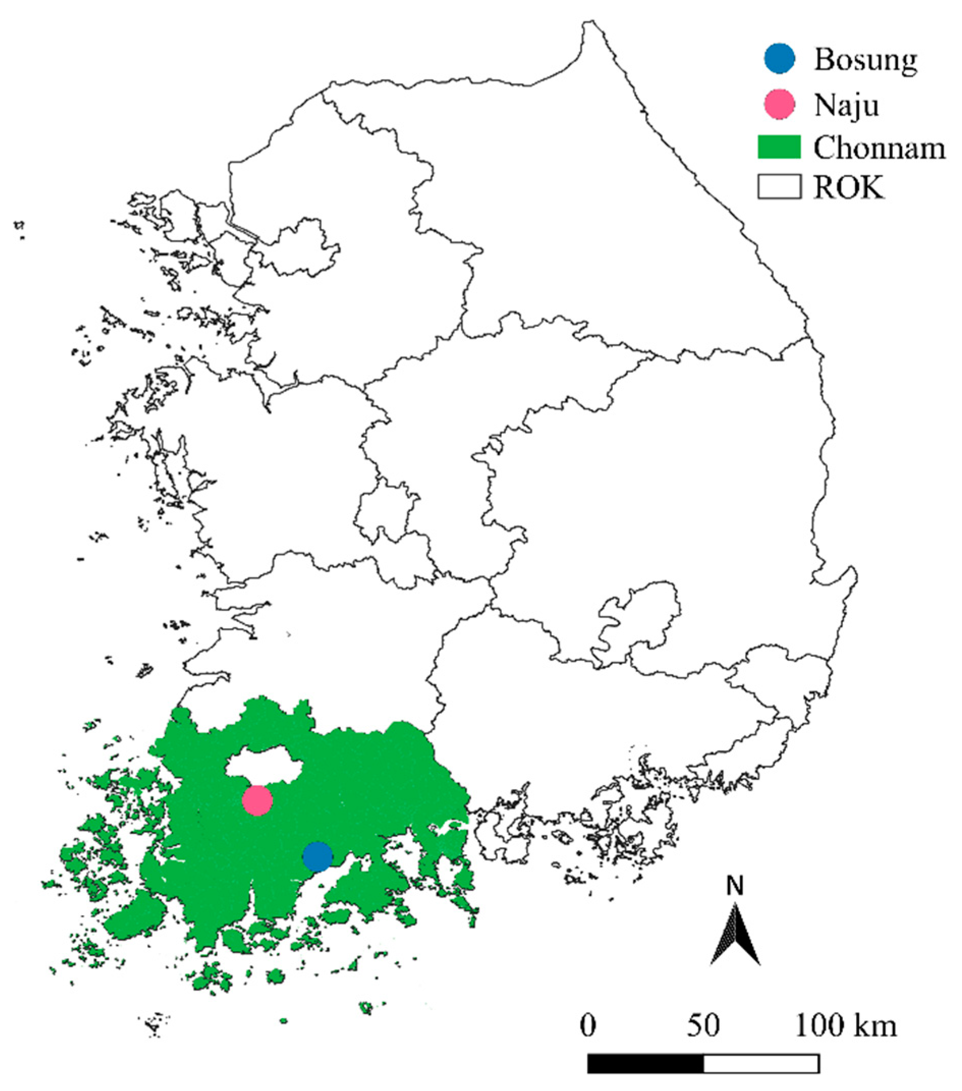
2.1. Experimental Field Data of Rice, Barley, and Soybean

Field experiments were conducted at AVS research facilities in Bosung and Naju, Chonnam Province, South Korea (Figure 1). The AVS in Bosung covers 2016 m2 (84 × 24 m), with a panel distance of 1.5 m at the height of 6 m. The AVS structure in Naju covers 3900 m2 (65 × 60 m) with a panel distance of 2.5 m at the height of 6 m. The panel slope of 35°, facing southeast, was designed to obtain a 35% solar radiation reduction rate. The panel slope of 30°, facing south, was intended to achieve a 28.9% solar radiation reduction rate.
The total provincial area of Chonnam is ~12,247 km2, situated in an inland region between latitudes 34° 17′ and 35° 29′ N, and longitudes 126° 5′ and 127° 46′ E. The 30-year average annual temperatures during the summer crop growing season, from May to October, in Chonnam ranged from ~12 °C to 15 °C, according to the Korea Meteorological Administration, KMA (https://data.kma.go.kr/, accessed on 1 November 2021). The average annual total precipitation for the equivalent period ranged from ~1200 to 1500 mm, with ~60% of it being received between June and September. The soil textures of the experimental areas were classified as an Entilsols loam at Naju and an Inceptisols sandy loam at Bosung based on the United States Department of Agriculture soil taxonomy. The Naju soil contains a total organic carbon of 12.3 g kg−1, total nitrogen of 1.0 g kg−1, available phosphate of 13.1 g kg−1, and the soil pH (in H2O) of 5.5. The Bosung soil contains a total organic carbon of 16.5 g kg−1, a total nitrogen of 1.2 g kg−1, an available phosphate of 12.7 g kg−1, and a soil pH in H2O of 5.8. Additional specific soil properties can be found in the Korea Soil Information System (http://soil.rda.go.kr/eng/, accessed on 1 November 2021) [31].
The field experiments were performed from 2019 to 2020 at the synthetic AVS facilities in Bosung and Naju to simulate barley (Hordeum vulgare), rice (Oryza sativa), and soybean (Glycine max) yields based on the determination of genetic coefficients of each crop cultivar (Table A1, Table A2 and Table A3). We chose two varieties of rice and barley and one variety of soybean among the available local crop cultivars bred by the National Institute of Crop Science (http://www.nics.go.kr/english/index.do, accessed on 1 November 2021). Paddy rice was transplanted on day of year (DOY) 162 of 2019 in Naju and DOY 162 of 2020 in Bosung. Barley was seeded on DOY 308 of 2019 in Bosung, while soybean was sown on DOY 167 of 2019 and 2020 in Naju. Each crop field was arranged as three randomized complete blocks. During the crop seasons, all the fields were managed with the typical N-P2O5-K2O fertilization of 80-70-35 kg ha−1 for barley, 90-45-57 kg ha−1 for rice, and 30-30-34 kg ha−1 for soybean, respectively. We estimated crop yields by measuring the grains harvested from sample plants in each experimental plot (2 m2, soybean and barley; 100 plants, rice). The plant samples for the yield estimation were harvested and measured at maturity in four replicates in each experimental unit. The rice plant samples were manually cut on DOY 265 for Chomeong-1, DOY 275 for Ilmi in 2019, and DOY 273 for Chomeong-1, DOY 280 for Ilmi in 2020. The Heenchal and Hopum barley cultivars were harvested for the yield estimation on DOY 156 in 2020. Daewon soybean was sampled on DOY 309 in 2019 and 297 in 2020. In addition, the weather data of the AVS-facilitated and open fields were obtained using separate sensors at five representative locations in each experimental block (i.e., north, south, east, west, and the center). The weather factors were measured using the following sensors: SQ-110 (Apogee Instruments Inc., Logan, UT, USA) for photosynthetically active radiation, SP-100 (Apogee Instruments Inc., Logan, UT, USA) for incident solar radiation, ATMOS-14 (METER Inc., Pullman, WA, USA) for temperature and humidity, and ECRN-100 (METER Inc., Pullman, WA, USA) for rainfall.

2.2. Crop Models

Crop models are theoretically designed and formulated to reproduce the field conditions of crop productivity, responding to diverse ecological, biological, and physical aspects (Figure A1). We employed CERES-Rice, CERES-Barley, and CROPGRO-Soybean from crop models available in the DSSAT package [24] to simulate the impacts of solar radiation reduction regimes on the yield of rice, barley, and soybean in Chonnam province, South Korea. These crop models, being designed as process-based management-level simulation models, can reproduce field conditions of crop morphogenesis and yield, soil water, and soil nutrient balance associated with crop growth. This study highlights the distinction between general field practice and our simulation research using the CERES-Rice, CERES-Barley, and CROPGRO-Soybean models.
Independent variables and parameters in the CERES and CROPGRO models comprise crop genetic coefficients, climate data, CO2 concentration, and chemical and physical soil data [32]. Daily solar radiation, maximum and minimum temperatures, and precipitation are the minimum variables for model simulations. The other required input parameters comprise crop genetic coefficients, physical and hydraulic soil characteristics, initial soil nitrogen and water conditions, and crop management records, such as planting date, planting depth, plant population, and the amounts and methods of irrigation and fertilizer applications. For example, there are eight genetic coefficients in CERES-Rice, seven genetic coefficients in CERES-Barley, and twelve genetic coefficients in CROPGRO-Soybean (Table A1, Table A2 and Table A3). These genetic coefficients are used to characterize the morphogenesis and yield-producing processes of the associated crop species.

2.3. Simulation of Crop Yield Variations

The CERES-Rice, CERES-Barley, and CROPGRO-Soybean models were calibrated and validated using the rice, barley, and soybean datasets obtained from the APS experimental fields in Bosung and Naju. The models in the GCSM were then applied to simulate the impacts of solar radiation reduction scenarios on these crops for the whole geographical area of Chonnam province, South Korea. Environmental variables and parameters used to reproduce the field conditions of rice, barley, and soybean yields in this study included (1) soil data, (2) climate data, (3) crop genetic coefficients, and (4) crop management metadata.
The GCSM system was established using the CERES-Rice, CERES-Barley, and CROPGRO-Soybean crop models. The GCSM scheme developed earlier [12,33] was further formulated to simulate the probable effects of solar radiation reduction regimes on regional geographical variations in rice, barley, and soybean yields. The GCSM system was programmed to run each crop model repeatedly, using pixel-based two-dimensional climate and soil data based on shell scripting in a Linux operating system (Figure 2). We also formulated the GCSM structure to manipulate model input conditions of interest, including crop cultivar choice, planting date, planting density, soil fertilization, and environmental changes (i.e., solar radiation, temperature, and CO2 concentration). The GCSM scheme allows the whole geographical territory to be assigned using a two-dimensional pixel array, with each pixel corresponding to 1 km2.
We used the grid-based two-dimensional soil data from digital soil maps (1:5000) for the whole Chonnam Province, South Korea, obtained from the National Academy of Agricultural Science, NAAS (http://soil.rda.go.kr/eng/, accessed on 1 November 2021). Grid-based climate data were also employed, which was projected using a dynamic downscaling procedure to establish high-resolution regional agro-climate indices using a regional climate model (i.e., Weather Research and Forecasting Model) by Ahn et al. [34]. Fifteen-year climate data (2011–15) with a 1-km ground resolution were employed as the baseline to simulate geographical variation in crop productivity using the GCSM system. We pre-processed and used the pixel-by-pixel soil data and the corresponding climate data as input for the crop models in the GCSM structure to project pixel-by-pixel crop productivity, which was designed and formulated in the earlier study [12]. The details of soil inventory have been explained by Hong et al. [31]. The soil data were used to establish soil input coefficients for the crop model of the GCSM system, based on the information gathered on selected soil properties, such as soil type and texture, adequate soil depth, and soil structure for each pixel of the region. We predetermined and constructed the eight probable soil input collections analytically for crop cultivation in Chonnam Province (Table 1). These soil input archives were prepared from the combined soil information using the generic soil input list of the DSSAT package. The GCSM system was designed to select one of the soil input inventories.

2.4. Statistical Analysis

We applied three assessment statistics to evaluate the crop modeling process of the yield simulation. The p-value from a two-sample t-test, root mean squared error (RMSE), and Nash–Sutcliffe model efficiency (NSE) were obtained [35]. NSE is a normalized indicator that identifies the relative magnitude of the simulated residual variance compared to the measured data variance; thus, it can verify how well the comparison plot of the simulated and measured data statistically agree to the 1:1 line. NSE values range from −∞ to 1. The closer the value is to one, the more dependent the model estimation precision. The nearer to zero, the lower the model estimate. Statisticians employ normalized NSE (NNSE) for advanced interpretation, allowing for the NSE measure in parameter estimation approaches used in model calibration. Thus, NSE = 1, 0, and −∞ correspond to NNSE = 1, 0.5, and 0, respectively.

3. Results

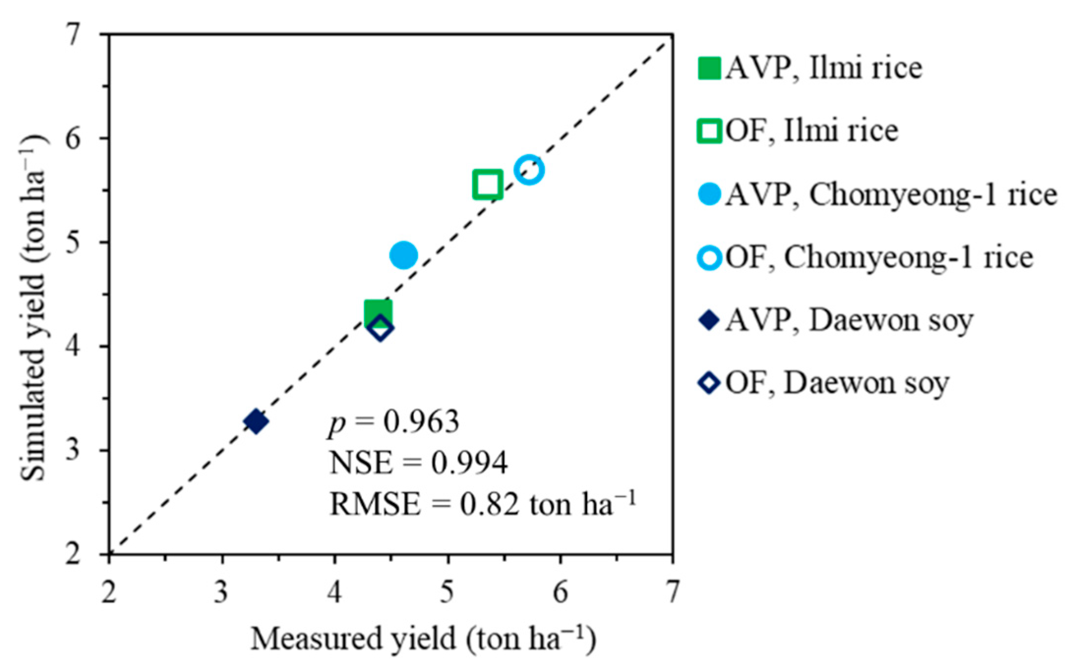
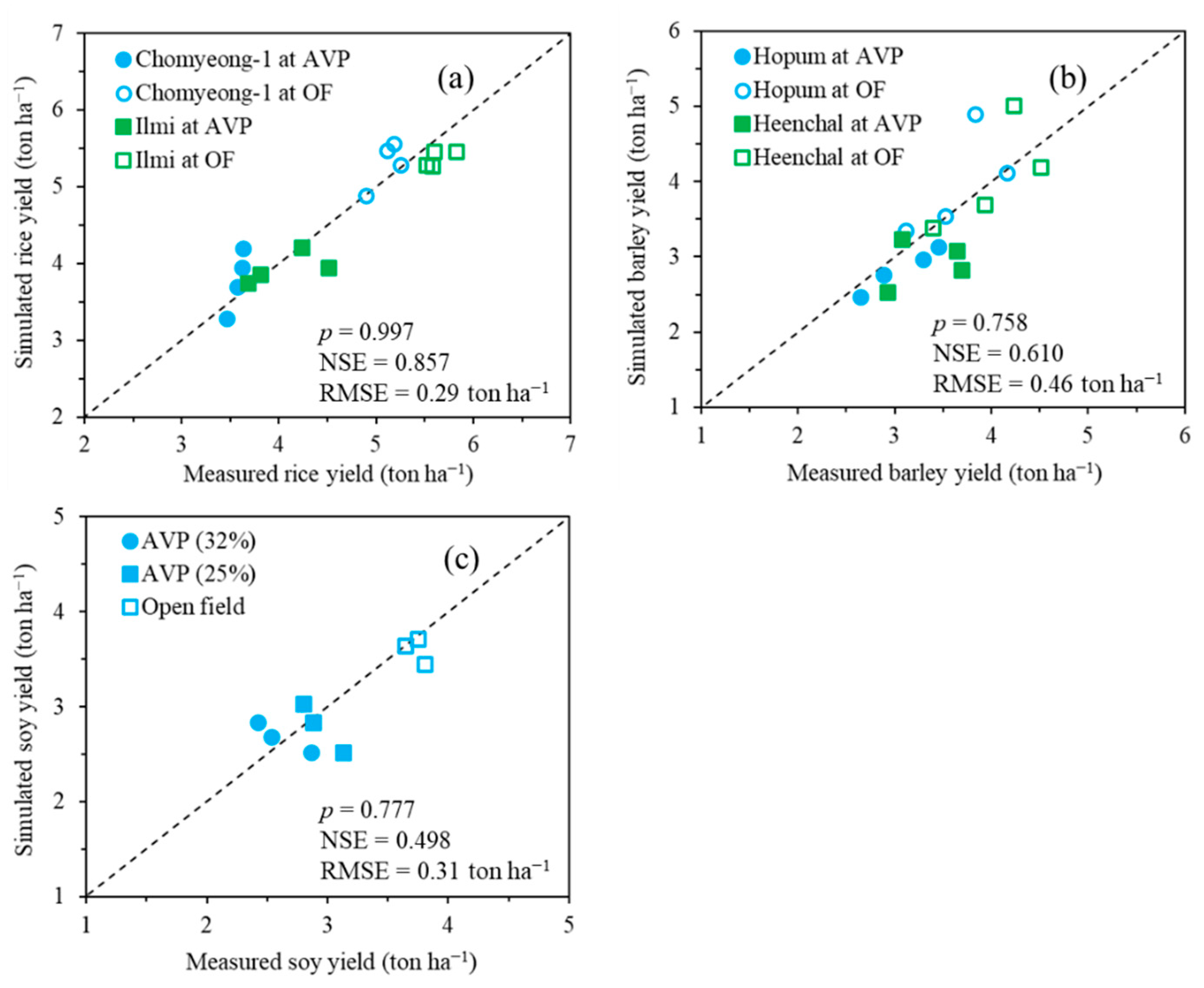
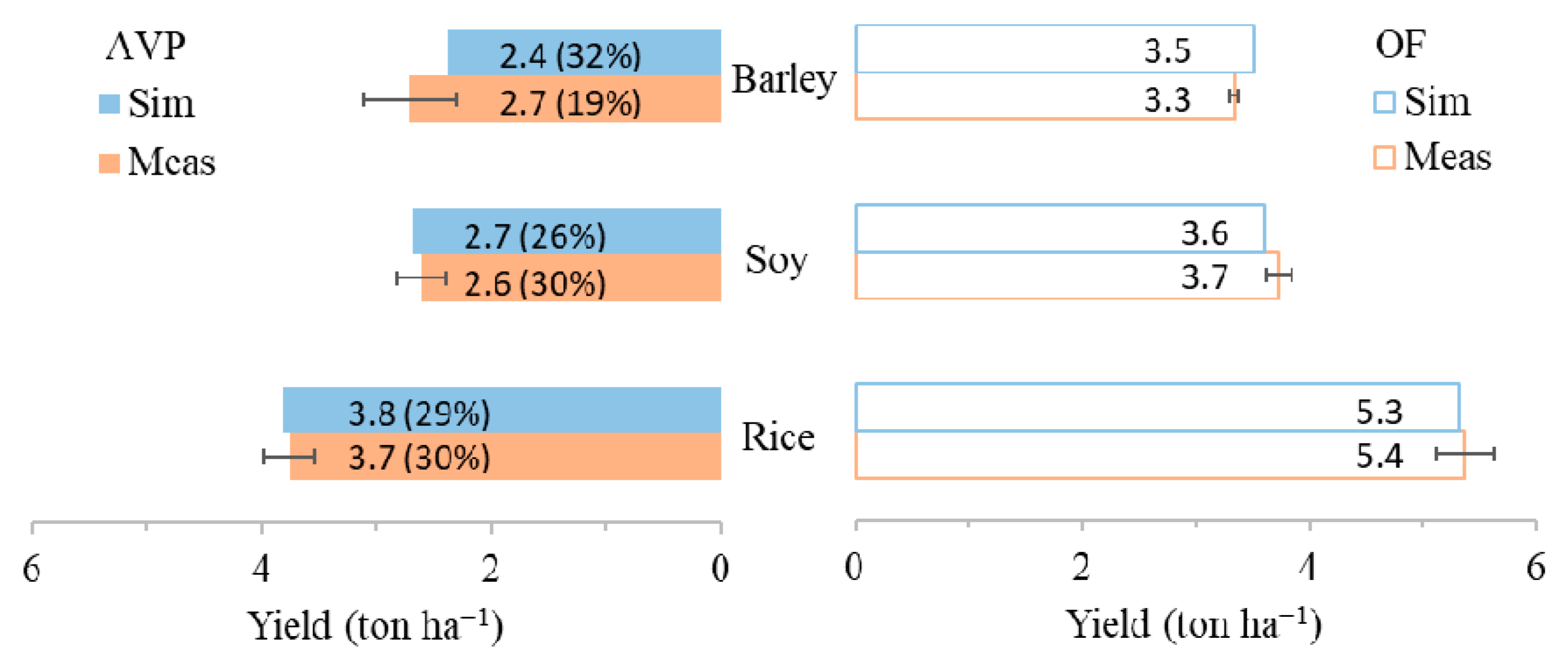
3.1. Simulation of Rice, Barley, and Soybean Yields

The CERES-rice, CECES-barley, and CROPGRO-soybean models reproduced field variations in rice, barley, and soybean yields with significant statistical agreements (Figure 3 and Figure 4). For example, in model calibration using the 2019 dataset, simulated crop yields agreed with the corresponding measured crop yields with a p-value of 0.963 according to a two-sample t-test, an NSE of 0.994, and an RMSE of 0.82-ton ha−1. In the model evaluation using the 2020 dataset, simulated crop yields significantly agreed with the measured crop yields, with p-values of 0.997, 0.758, and 0.777; NSE values of 0.857, 0.610, and 0.498; and RMSEs of 0.29, 0.46, and 0.31-ton 10a−1 for paddy rice, barley, and soybean, respectively. All in all, we found that the crop models closely simulated the crop yields in agreement with the corresponding measurements treated with AVPs compared to open fields, showing its capability of reproducing yield decreases in response to solar radiation declines due to the AVPs (Figure 5).
Paddy rice and barley yields declined curvilinearly with a slow phase, up to a solar radiation reduction of 60%, while the soybean yield decreased linearly at a relatively rapidly falling scale (Figure 6). For example, the paddy rice, barley, and soybean yields declined by 18.1, 14.1, and 20.8% under a 20% solar radiation reduction regime compared to the baseline (100% solar radiation). These crop yields decreased by 27.1, 19.9, and 32.4% under a 30% solar radiation reduction plan.

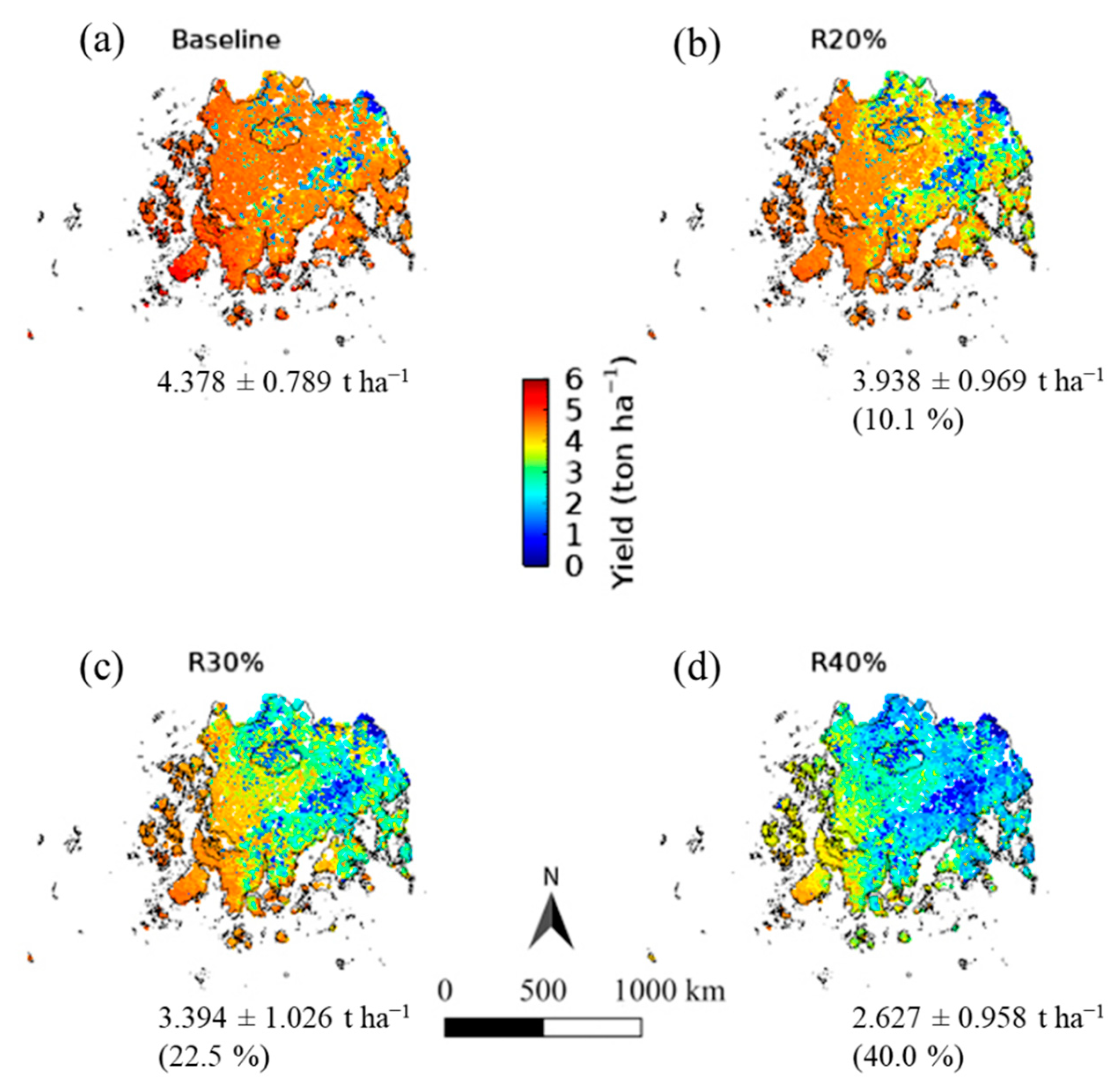
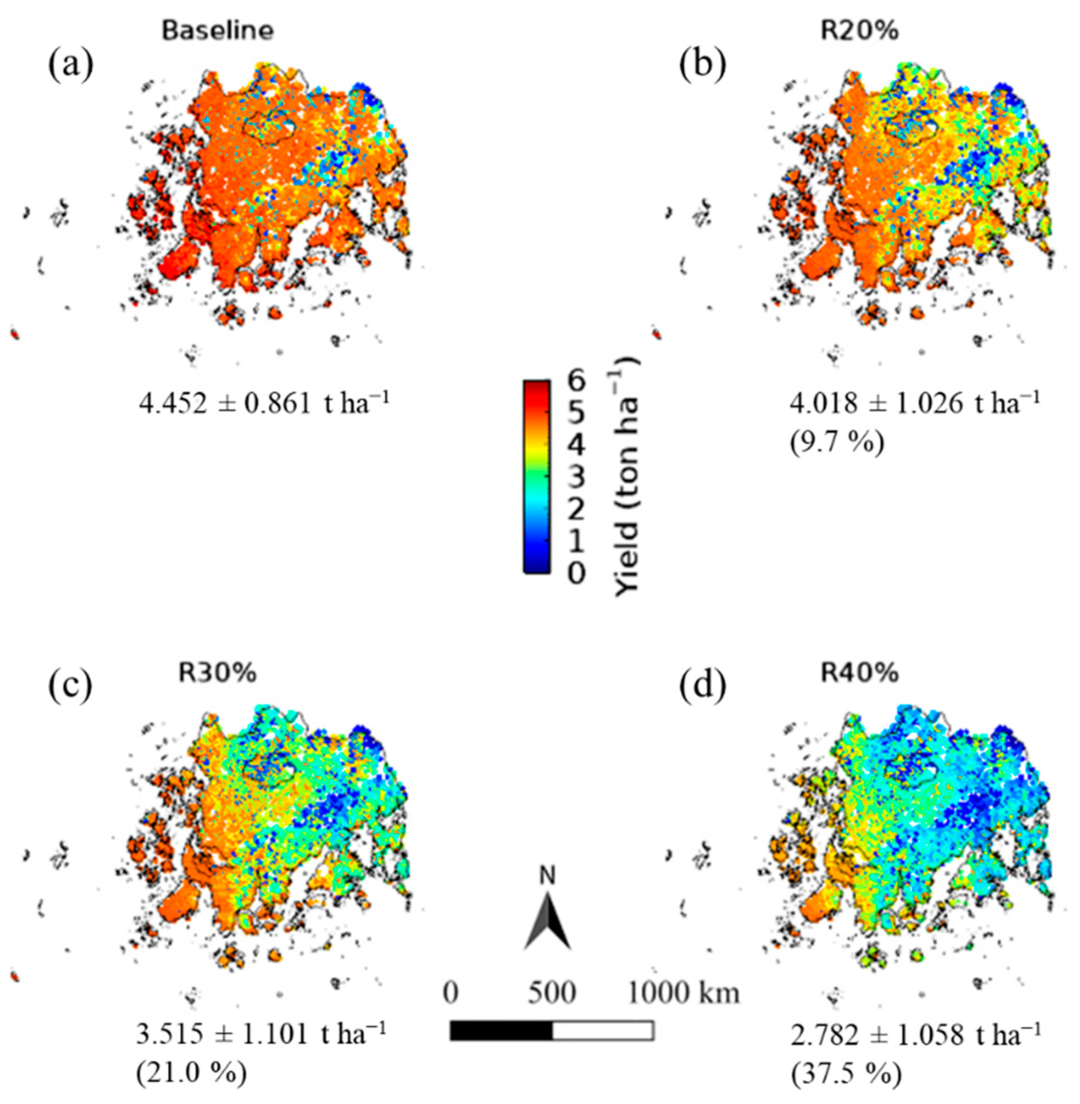
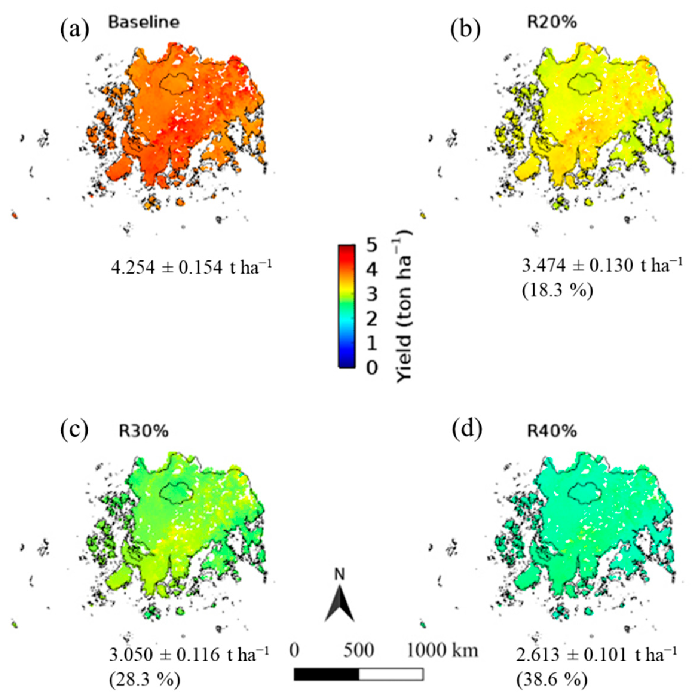
3.2. Simulation of Geographical Yield Variations Due to Solar Radiation Reductions

We also employed the CERES-rice, CERES-barley, and CROPGRO-soybean models in the GSCM system to simulate the potential influences of the AVP regime on yields for these crops in the whole geographical area of Chonnam province, South Korea. As a result, paddy rice, barley, and soybean yield for the solar radiation scenarios of 20, 30, and 40% declines were projected. According to the procedures, Chomyeong rice yields decreased by 9.7, 21.0, and 37.5% under 20, 30, and 40% reductions, respectively (Figure 7). Heenchal barley yields decreased by 8.3, 13.5, and 19.5% under 20, 30, and 40% reductions, respectively (Figure 8). Daewon soybean yields decreased by 18.3, 28.3, and 38.6% under 20, 30, and 40% reductions, respectively (Figure 9). The yield reductions of Ilmi rice were similar to those of Chomyeong (Figure A2). Therefore, it appears that there was not much varietal variation in the yield decline rate in response to the solar radiation reduction regime. Meanwhile, the crop yields estimated were relatively higher in coastal areas and lower in inner mountainous territories.

4. Discussion

The current study successfully calibrated and validated CERES-rice, CERES-barley, and CROPGRO-soybean models for the simulation of rice, barley, and soybean yields grown under the AVS experimental fields, followed by the reproduction of these crop yields in the geographical Chonnam region of South Korea. These models demonstrated effectiveness in these study results and have also been proven useful in various research aspects of scientific interest to deliver more sophisticated crop productivity matters. For example, endeavors toward further progress could include crop morphogenesis study practices and an investigation of plant-water-soil-nutrient interactions [36,37]. We presume that the crop modeling approach can hypothetically fill a gap between the experimental study findings and the practical ecosystem requirement for the optimal AVS, which allows for the development of a crop modeling regime as a decision support system.
Crop models have been applied in various agricultural ecosystems as decision support or research tools. The model applications include, but are not limited to, crop cultivation and productivity management [38,39,40], impacts of climate change [16,41], and fusion with remote sensing [42,43]. However, there have been no reports on the use of a crop model to simulate crop production aspects with AVS field conditions, to the best of our knowledge. Here, we demonstrated that the crop modeling methodology could well reproduce the field conditions of crop yield under AVPs. It is reported that crop yield reduction issues in the AVS fields are attributed to solar radiation declines caused by solar panels [2,4]. Therefore, some efforts to quantify crop productivity due to the solar radiation declines and address the associated challenges are required. Our study also presented that the crop models could project yield responses to solar radiation reductions (Figure 6), demonstrating that the crop models could be employed as a decision support tool. A well-calibrated crop model can be a practical tool to quantify probable influences on various scenarios, such as the solar radiation reduction issue, and to help establish an optimum management option [36]. Feasible measures to overcome the possible effects of solar radiation reduction scenarios on crop production include the selection of optimum cultivars as well as improvement through breeding and different cultivation and management options (e.g., planting date and density and associated fertilization).
We further formulated a GCSM structure established previously [12,33] to simulate the possible effects of solar radiation reduction regimes on geographical changes in rice, barley, and soybean yields. As a result, we effectively characterized the two-dimensional variations in these crop yields within the geographical areas of the province, indicating higher crop yields in coastal regions and lower crop yields in inner mountainous territories. Thus, to the best of our knowledge, this study is the first to simulate the impacts of solar radiation reduction scenarios on rice, barley, and soybean with a fine grid (1 km)-based regional yield projection. Meanwhile, it is assumed that there are typically two-dimensional variation factors within the AVP facility environment during a day in the crop season, mainly attributed to the altitude and direction changes of solar radiations [4,29,44]. Thus, the solar radiation variation is assumed to involve subsequent crop productivity variation, producing yield reductions. Consequently, it would be helpful to design a two-dimensional crop modeling system to project spatiotemporal crop productivity with a fine grid scale to determine local variations in crop production.
The AVS facility of the Naju study site had 161 units of 405 watts (W) with an installation cost of $0.35 per W, generating the total electricity at 88.1 and 110.1 kWh per day with 25.6 and 32% solar radiation shading schemes in the case of the mono-facial solar modules [45]. According to the corresponding report, the crop production profits under the AVP varied depending on crops, estimating ~30 and 38 thousand dollars per ha at 25.6 and 32% solar radiation shadings for soybean when adopting the system marginal price and renewable energy credit policies of the South Korean government [46,47]. Therefore, renewable energy generation likely compensates for crop yield declines due to the solar radiation reductions. However, while it is out of the current study scope, we assume that the crop production profits estimate can be more advanced by employing a decision support system approach formulated with a crop modeling scheme than the field experiment-based results mentioned above. This speculation could be referenced from earlier studies, e.g., the impacts of climate change on cropping systems and irrigation and agricultural resource management [36,38,39]. Therefore, future studies should be directed toward developing the modeling approach as a decision support system considering various AVS and the corresponding crop management options.

5. Conclusions

The results of the current study proved that the CERES-Rice, CERES-Barley, and CROPGRO-Soybean models in the DSSAT package could be used in discovering the effects of solar radiation reductions on rice, barley, and soybean productions for the climate of Chonnam Province, South Korea. Moreover, we also demonstrated that the established GCSM scheme using these crop models could simulate geospatial variations in crop productivity under different solar radiation reduction scenarios. Therefore, we believe that the GCSM structure formulated in this study could be efficiently employed to simulate the influences of solar radiation reductions on staple crops, reproducing geographical variations. Furthermore, the modeling methodology allows for an exploration of practical interpretations for improving food security measures. However, the system needs further improvement to be helpful as an objective tool for scientists and stakeholders. The limitation of the current study is that the crop models were calibrated using the partial AVS experimental dataset. Further studies using additional experimental datasets (e.g., examining different AVP types and the associated crop productivity practices) would add substantial scientific values. Furthermore, a decision support system should be ultimately developed based on formulating a modeling methodology utilizing these datasets.

Author Contributions

J.K. designed the research and wrote the first draft; J.C. (Jaeil Cho), C.-Y.Y., K.-N.A., and D.-K.K. obtained data; J.K. and J.C. (Jinsil Choi) analyzed the data; J.K. and J.-O.B. developed the modeling system; all authors contributed to organizing the final draft. All authors have read and agreed to the published version of the manuscript.

Funding

This research was supported by Chonnam National University (Grant number: 2018-3251), Gwangju, Jeollanamdo Agricultural Research and Extension Services, Naju, Chonnam Province, and KEPCO Research Institute, Daejeon, Republic of Korea. In addition, partial financial assistance was provided by the Cooperative Research Program for Agriculture Science and Technology Development (Project No. PJ01476803) from the Rural Development Administration, Republic of Korea.

Acknowledgments

The authors would like to thank Editage (www.editage.co.kr, accessed on 30 November 2021) for English language editing.

Conflicts of Interest

The authors declare no conflict of interest.

Appendix A

Table A1. Genetic coefficients of two rice cultivars.
Coeff. IlmiChomyeong-1
P1320.0320.0
P2O12.812.8
P2R20.035.0
P5530.0500.0
G165.065.0
G20.0220.021
G31.21.2
G41.01.0
PHINT77.083.0
P1, time length from seedling emergence during which rice is not responsive to variations in photoperiod (growing degree days (GDD) in C above a base temperature of 9 °C); P2O, critical photoperiod (the longest day length) where the plant development happens at a maximum rate (in hours); P2R, extent to which phasic development leading to panicle initiation is delayed for each hour increase in photoperiod above P20 (expressed as GDD in °C); P5, time period from beginning of grain filling (3 to 4 days after flowering) to physiological maturity with a base temperature of 9 °C (GDD in °C); G1, probable spikelet number parameter as valued from the number of spikelets per g of main culm dry weight (less leaf blades and sheaths, plus spikes) at anthesis; G2, single grain weight (g) under perfect growing environments, i.e., non-limiting light, water, nutrients, and absence of pests and diseases; G3, tillering parameter (scaler value) relative to IR64 cultivar under ideal conditions; G4, temperature tolerance coefficient; PHINT, period between following leaf tip appearances (C day). The parameter acronyms and descriptions are from the genetic coefficients of rice in the DSSAT package v4.6 [24].
Table A2. Genetic coefficients of two barley cultivars.
Generic Coefficient HeenChalHopum
P1V1010
P1D2020
P5220220
G12020
G22423
G31.51.5
PHINT9190
P1V, optimum temperature needed for vernalization (day); P1D, photoperiod response (% reduction in the rate per 10 h drop in the photoperiod); P5, grain filling (excluding lag) phase period (°C day); G1, grain number per unit canopy weight at anthesis; G2, normal grain size under optimum conditions (mg); G3, normal, non-stressed mature tiller weight (g); PHINT, interval between successive leaf tip appearances (°C day). The parameter acronyms and descriptions are from the genetic coefficients of barley in the DSSAT package v4.6 [24].
Table A3. Genetic coefficients of Daewon soybean cultivar.
Coeff. Daewon
CSDL12.02
PPSEN0.266
EM-FL13.3
FL-SH12.0
FL-SD18.5
SD-PM39.5
FL-LF26.0
LFMAX1.02
SLAVR390
SIZLF180
WTPSD0.19
SFPDV24.0
CSDL, critical short day period below which reproductive development continues with no day length influence for short-day plants (hour); PPSEN, slope of the comparative response of development to photoperiod with time (positive for short day plants) (per hour); EM-FL, time between plant seedling emergence and initial flowering (R1) (photo-thermal days); FL-SH, time between first flower and first pod (R3) (photo-thermal days); FL-SD, time between first flower and first seed (R5) (photo-thermal days); SD-PM, time between first seed (R5) and physiological maturity (R7) (photo-thermal days); FL-LF, time between first flower (R1) and end of leaf expansion (photo-thermal days); LFMAX, maximum leaf photosynthesis rate at 30 °C, 350 vpm CO2, and high solar radiation (mg (CO2) m−2 s−1); SLAVR, specific leaf area of the variety under normal growth conditions (cm2 g−1); SIZLF, maximum size of whole leaf (three leaflets) (cm2); WTPSD, maximum weight per seed (g); SFPDV, average seed per pod under normal growing conditions (# per pod). The parameter acronyms and descriptions are from the genetic coefficients of soybean in the DSSAT package v4.6 [24].
Figure A1. Crop model concepts (modified from Lövenstein, et al. [48]).
Energies 14 08463 g0a1
Figure A2. Maps of simulated Ilmi rice yields under the solar radiation reductions (R) of 20% (b), 30% (c), and 40% (d) compared to the baseline (a) in Chonnam province, South Korea. The values in the parentheses represent the percentage of yield reduction in comparison with the baseline yield.
Energies 14 08463 g0a2

References

  1. Barron-Gafford, G.A.; Pavao-Zuckerman, M.A.; Minor, R.L.; Sutter, L.F.; Barnett-Moreno, I.; Blackett, D.T.; Thompson, M.; Dimond, K.; Gerlak, A.K.; Nabhan, G.P.; et al. Agrivoltaics provide mutual benefits across the food–energy–water nexus in drylands. Nat. Sustain. 2019, 2, 848–855. [Google Scholar] [CrossRef]
  2. Dupraz, C.; Marrou, H.; Talbot, G.; Dufour, L.; Nogier, A.; Ferard, Y. Combining solar photovoltaic panels and food crops for optimising land use: Towards new agrivoltaic schemes. Renew. Energy 2011, 36, 2725–2732. [Google Scholar] [CrossRef]
  3. AL-agele, H.A.; Proctor, K.; Murthy, G.; Higgins, C. A Case Study of Tomato (Solanum lycopersicon var. Legend) Production and Water Productivity in Agrivoltaic Systems. Sustainability 2021, 13, 2850. [Google Scholar] [CrossRef]
  4. Marrou, H.; Guilioni, L.; Dufour, L.; Dupraz, C.; Wery, J. Microclimate under agrivoltaic systems: Is crop growth rate affected in the partial shade of solar panels? Agric. For. Meteorol. 2013, 177, 117–132. [Google Scholar] [CrossRef]
  5. Cho, Y.; Kim, H.; Jo, E.; Oh, D.; Jeong, H.; Yoon, C.; An, K.; Cho, J. Effect of Partial Shading by Agrivoltaic Systems Panel on Electron Transport Rate and Non-photochemical Quenching of Crop. Korean J. Agric. For. Meteorol. 2021, 23, 100–107. [Google Scholar]
  6. Klerkx, L.; Begemann, S. Supporting food systems transformation: The what, why, who, where and how of mission-oriented agricultural innovation systems. Agric. Syst. 2020, 184, 102901. [Google Scholar] [CrossRef]
  7. de Boon, A.; Sandström, C.; Rose, D.C. Governing agricultural innovation: A comprehensive framework to underpin sustainable transitions. J. Rural. Stud. 2021, 23, 100–107. [Google Scholar] [CrossRef]
  8. Faria, J.R.; Mixon, F.G. Farmer-entrepreneurs, agricultural innovation, and explosive research and development cycles. Adm. Sci. 2016, 6, 13. [Google Scholar] [CrossRef] [Green Version]
  9. Yousefi-Babadi, A.; Bozorgi-Amiri, A.; Tavakkoli-Moghaddam, R. Sustainable facility relocation in agriculture systems using the GIS and best–worst method. Kybernetes 2021. ahead-of-print. [Google Scholar] [CrossRef]
  10. Lombardi, M.; Costantino, M. A Social Innovation model for reducing food waste: The case study of an Italian non-profit organization. Adm. Sci. 2020, 10, 45. [Google Scholar] [CrossRef]
  11. Dospinescu, N.; Dospinescu, O.; Tatarusanu, M. Analysis of the influence factors on the reputation of food-delivery companies: Evidence from Romania. Sustainability 2020, 12, 4142. [Google Scholar] [CrossRef]
  12. Ko, J.; Tim Ng, C.; Jeong, S.; Kim, J.-H.; Lee, B.; Kim, H.-Y. Impacts of regional climate change on barley yield and its geographical variation in South Korea. Int. Agrophysics 2019, 33, 81–96. [Google Scholar] [CrossRef]
  13. Lobell, D.B.; Schlenker, W.; Costa-Roberts, J. Climate Trends and Global Crop Production Since 1980. Science 2011, 333, 616–620. [Google Scholar] [CrossRef] [Green Version]
  14. Palosuo, T.; Hoffmann, M.P.; Rötter, R.P.; Lehtonen, H.S. Sustainable intensification of crop production under alternative future changes in climate and technology: The case of the North Savo region. Agric. Syst. 2021, 190, 103135. [Google Scholar] [CrossRef]
  15. Ko, J.; Kim, H.-Y.; Jeong, S.; An, J.-B.; Choi, G.; Kang, S.; Tenhunen, J. Potential impacts on climate change on paddy rice yield in mountainous highland terrains. J. Crop. Sci. Biotechnol. 2014, 17, 117–126. [Google Scholar] [CrossRef]
  16. Kim, H.Y.; Ko, J.; Kang, S.; Tenhunen, J. Impacts of climate change on paddy rice yield in a temperate climate. Glob. Chang. Biol. 2013, 19, 548–562. [Google Scholar] [CrossRef]
  17. Ahuja, L.R.; Rojas, K.W.; Hanson, J.D.; Shaffer, M.J.; Ma, L. Root Zone Water Quality Model: Modeling Management Effects on Water Quality and Crop Production; Water Resources Publications, LLC: Highland Ranch, CO, USA, 2000. [Google Scholar]
  18. Kirschbaum, M.U.F. Forest growth and species distribution in a changing climate. Tree Physiol. 2000, 20, 309–322. [Google Scholar] [CrossRef]
  19. McCown, R.L.; Hammer, G.L.; Hargreaves, J.N.G.; Holzworth, D.P.; Freebairn, D.M. APSIM: A novel software system for model development, model testing and simulation in agricultural systems research. Agric. Syst. 1996, 50, 255–271. [Google Scholar] [CrossRef]
  20. Brisson, N.; Gary, C.; Justes, E.; Roche, R.; Mary, B.; Ripoche, D.; Zimmer, D.; Sierra, J.; Bertuzzi, P.; Burger, P.; et al. An overview of the crop model stics. Eur. J. Agron. 2003, 18, 309–332. [Google Scholar] [CrossRef]
  21. Ma, L.; Hoogenboom, G.; Ahuja, L.; Nielsen, D.; Ascough, J. Development and evaluation of the RZWQM-CROPGRO hybrid model for soybean production. Agron. J. 2005, 97, 1172–1182. [Google Scholar] [CrossRef] [Green Version]
  22. Williams, J.R. The Erosion-Productivity Impact Calculator (EPIC) Model: A Case History. Philos. Trans. Biol. Sci. 1990, 329, 421–428. [Google Scholar]
  23. Hijmans, R.J.; Guiking-Lens, I.; Van Diepen, C. WOFOST 6.0: User’s Guide for the WOFOST 6.0 Crop Growth Simulation Model; DLO Winand Staring Centre: Wageningen, The Netherlands, 1994; p. 145. [Google Scholar]
  24. Jones, J.W.; Hoogenboom, G.; Porter, C.H.; Boote, K.J.; Batchelor, W.D.; Hunt, L.; Wilkens, P.W.; Singh, U.; Gijsman, A.J.; Ritchie, J.T. The DSSAT cropping system model. Eur. J. Agron. 2003, 18, 235–265. [Google Scholar] [CrossRef]
  25. Singh, U.; Ritchie, J.; Thornton, P. CERES-Cereal Model for Wheat, Maize, Sorghum, Barley, and Pearl Millet; Agronomy Abstracts: Madison, WI, USA, 1991; p. 78. [Google Scholar]
  26. Boote, K.J.; Jones, J.W.; Hoogenboom, G.; Pickering, N. Simulation of crop growth: CROPGRO model. Agric. Syst. Modeling Simul. 1998, 18, 651–692. [Google Scholar]
  27. Singh, U.; Matthews, R.B.; Griffin, T.S.; Ritchie, J.T.; Hunt, L.A.; Goenaga, R. Modeling growth and development of root and tuber crops. In Understanding Options for Agricultural Production; Tsuji, G.Y., Hoogenboom, G., Thornton, P.K., Eds.; Springer: Dordrecht, The Netherlands, 1998; pp. 129–156. [Google Scholar] [CrossRef]
  28. Kim, J.; Park, J.; Hyun, S.; Fleisher, D.H.; Kim, K.S. Development of an automated gridded crop growth simulation support system for distributed computing with virtual machines. Comput. Electron. Agric. 2020, 169, 105196. [Google Scholar] [CrossRef]
  29. Dinesh, H.; Pearce, J.M. The potential of agrivoltaic systems. Renew. Sustain. Energy Rev. 2016, 54, 299–308. [Google Scholar] [CrossRef] [Green Version]
  30. Thornley, J.H.; Johnson, I.R. Plant and Crop Modelling: A Mathematical Approach to Plant and Crop Physiology; Clarendon Press: Oxford, UK, 1990. [Google Scholar]
  31. Hong, S.Y.; Zhang, Y.-S.; Hyun, B.-K.; Sonn, Y.-K.; Kim, Y.-H.; Jung, S.-J.; Park, C.-W.; Song, K.-C.; Jang, B.-C.; Choe, E.-Y. An introduction of Korean soil information system. Korea J. Soil Sci. Fert. 2009, 42, 21–28. [Google Scholar]
  32. Harb, O.; Abd El-Hay, G.; Hager, M.; Abou El-Enin, M. Calibration and validation of DSSAT V. 4.6. 1, CERES and CROPGRO models for simulating no-tillage in Central Delta, Egypt. Agrotechnology 2016, 5, 2. [Google Scholar]
  33. Kim, H.-Y.; Ko, J.; Jeong, S.; Kim, J.-H.; Lee, B. Geospatial delineation of South Korea for adjusted barley cultivation under changing climate. J. Crop. Sci. Biotechnol. 2017, 20, 417–427. [Google Scholar] [CrossRef]
  34. Ahn, J.; Hur, J.; Shim, K. A simulation of agro-climate index over the Korean peninsula using dynamical downscaling with a numerical weather prediction model. Korean J. Agric. For. Meteorol. 2010, 12, 1–10. [Google Scholar] [CrossRef]
  35. Nash, J.E.; Sutcliffe, J.V. River flow forecasting through conceptual models part I—A discussion of principles. J. Hydrol. 1970, 10, 282–290. [Google Scholar] [CrossRef]
  36. Ko, J.; Ahuja, L.R.; Saseendran, S.; Green, T.R.; Ma, L.; Nielsen, D.C.; Walthall, C.L. Climate change impacts on dryland cropping systems in the Central Great Plains, USA. Clim. Chang. 2012, 111, 445–472. [Google Scholar] [CrossRef]
  37. Ko, J.; Ahuja, L.; Kimball, B.; Anapalli, S.; Ma, L.; Green, T.R.; Ruane, A.C.; Wall, G.W.; Pinter, P.; Bader, D.A. Simulation of free air CO2 enriched wheat growth and interactions with water, nitrogen, and temperature. Agric. For. Meteorol. 2010, 150, 1331–1346. [Google Scholar] [CrossRef]
  38. Ko, J.; Piccinni, G.; Steglich, E. Using EPIC model to manage irrigated cotton and maize. Agric. Water Manag. 2009, 96, 1323–1331. [Google Scholar] [CrossRef]
  39. Mauget, S.A.; Ko, J. A two-tier statistical forecast method for agricultural and resource management simulations. J. Appl. Meteorol. Climatol. 2008, 47, 1573–1589. [Google Scholar] [CrossRef]
  40. Shin, T.; Ko, J.; Jeong, S.; Shawon, A.R.; Lee, K.D.; Shim, S.I. Simulation of Wheat Productivity Using a Model Integrated With Proximal and Remotely Controlled Aerial Sensing Information. Front. Plant Sci. 2021, 12, 446. [Google Scholar] [CrossRef] [PubMed]
  41. Rosenzweig, C.; Elliott, J.; Deryng, D.; Ruane, A.C.; Müller, C.; Arneth, A.; Boote, K.J.; Folberth, C.; Glotter, M.; Khabarov, N.; et al. Assessing agricultural risks of climate change in the 21st century in a global gridded crop model intercomparison. Proc. Natl. Acad. Sci. USA 2014, 111, 3268–3273. [Google Scholar] [CrossRef] [Green Version]
  42. Jeong, S.; Ko, J.; Kang, M.; Yeom, J.; Ng, C.T.; Lee, S.-H.; Lee, Y.-G.; Kim, H.-Y. Geographical variations in gross primary production and evapotranspiration of paddy rice in the Korean Peninsula. Sci. Total. Environ. 2020, 714, 136632. [Google Scholar] [CrossRef]
  43. Huang, J.; Gómez-Dans, J.L.; Huang, H.; Ma, H.; Wu, Q.; Lewis, P.E.; Liang, S.; Chen, Z.; Xue, J.-H.; Wu, Y.; et al. Assimilation of remote sensing into crop growth models: Current status and perspectives. Agric. For. Meteorol. 2019, 276–277, 107609. [Google Scholar] [CrossRef]
  44. Armstrong, A.; Ostle, N.J.; Whitaker, J. Solar park microclimate and vegetation management effects on grassland carbon cycling. Environ. Res. Lett. 2016, 11, 074016. [Google Scholar] [CrossRef] [Green Version]
  45. Kim, S.; Kim, S.; Yoon, C.-Y. An efficient structure of an agrophotovoltaic system in a temperate climate region. Agronomy 2021, 11, 1584. [Google Scholar] [CrossRef]
  46. Corporation, K.E.P. A Price of the System Marginal Price. Available online: https://home.kepco.co.kr/kepco/main.do (accessed on 9 December 2021).
  47. Exchange, K.P. A Price of the Renewable Energy Certificate. Available online: https://onerec.kmos.kr/portal/index.do (accessed on 9 December 2021).
  48. Lövenstein, H.; Rabbinge, R.; van Keulen, H. World Food Production, Textbook 2: Biophysical Factors in Agricultural Production; Wageningen University & Research: Wageningen, The Netherlands, 1992. [Google Scholar]
Figure 1. Map of the study sites of Naju and Bosung in Chonnam Province, Republic of Korea (ROK).
Energies 14 08463 g001
Figure 2. Geospatial crop simulation modeling scheme using the CERES-Rice, CERES-Barley, and CROPGRO-Soybean models in the DSSAT package.
Energies 14 08463 g002
Figure 3. Simulated and measured paddy rice and soybean yields under agro-photovoltaic panels (AVP) and at open fields in Jonnam Agricultural Research and Extension Services, Naju, South Korea, in 2019. NSE, p, and RMSE represent statistical indices of Nash–Sutcliffe model efficiency, the p-value from a paired t-test, and root mean squared error, respectively.
Energies 14 08463 g003
Figure 4. Simulated and measured yields of rice (a), barley (b), and soybean (c) under agro-photovoltaic panels (AVP) with 32% and 25% shade and open fields in Jonnam Agricultural Research and Extension Services, Naju, South Korea, in 2020. NSE, p, and RMSE represent statistical indices of Nash–Sutcliffe model efficiency, the p-value from a paired t-test, and root mean squared error, respectively.
Energies 14 08463 g004
Figure 5. Simulated versus measured barley, soybean, and rice yields grown under the agro-photovoltaic panels (AVP) and in open fields (OF). The values in the parentheses represent the percentage of reduction rates for the AVP crop yields compared to the OF crop yields.
Energies 14 08463 g005
Figure 6. Yield responses of rice (a), barley (b), and soybean (c) to different ratios of solar radiation amounts during the crop growing seasons.
Energies 14 08463 g006
Figure 7. Maps of simulated Chomyeong rice yields under the solar radiation reductions (R) of 20% (b), 30% (c), and 40% (d) compared to the baseline (a) in Chonnam province, South Korea. The values in the parentheses represent the percentage of yield reduction in comparison with the baseline yield.
Energies 14 08463 g007
Figure 8. Maps of simulated Heenchal barley yields under the solar radiation reductions (R) of 20% (b), 30% (c), and 40% (d) compared to the baseline (a) in Chonnam province, South Korea. The values in the parentheses represent the percentage yield reduction in comparison with the baseline yield.
Energies 14 08463 g008
Figure 9. Maps of simulated Daewon soybean yields under the solar radiation reductions (R) of 20% (b), 30% (c), and 40% (d) compared to the baseline (a) in Chonnam province, South Korea. The values in the parentheses represent the percentage yield reduction in comparison with the baseline yield.
Energies 14 08463 g009
Table 1. Selected properties of the generic soil input list of the DSSAT package v4.6 used in this study [12].
Soil IDTextureDepth
(cm)
AlbedoDrainage Rate
(Fraction Day−1)
Soil Water (cm3 cm−3)
CLLDUL
IB00000002Medium silty clay1500.110.20.2280.385
IB00000003Shallow silty clay600.110.10.2280.385
IB00000005Medium silty loam1500.120.30.1080.218
IB00000006Shallow silty loam600.120.20.1080.218
IB00000008Medium sandy loam1500.130.50.0520.176
IB00000009Shallow sandy loam600.130.40.0520.176
IB00000011Medium sand1500.150.50.0240.096
IB00000012Shallow sand600.150.40.0240.096
† Volumetric water content of the topsoil averaged among 5, 15, and 30 cm at the crop lower limit (CLL) and at the drained upper limit (DUL), respectively.
Publisher’s Note: MDPI stays neutral with regard to jurisdictional claims in published maps and institutional affiliations.

