Fault Coverage-Aware Metrics for Evaluating the Reliability Factor of Solar Tracking Systems

Abstract

This paper presents a mathematical approach for determining the reliability of solar tracking systems based on three fault coverage-aware metrics which use system error data from hardware, software as well as in-circuit testing (ICT) techniques, to calculate a solar test factor (STF). Using Euler’s named constant, the solar reliability factor (SRF) is computed to define the robustness and availability of modern, high-performance solar tracking systems. The experimental cases which were run in the Mathcad software suite and the Python programming environment show that the fault coverage-aware metrics greatly change the test and reliability factor curve of solar tracking systems, achieving significantly reduced calculation steps and computation time.

1. Introduction

The most abundant form of energy on our planet is incontestably the Sun. Despite dropping technology costs and free sunlight, conventional companies have been reluctant to use photovoltaic (PV) panels such as those installed on residences’ rooftops for large-scale projects. Concerning this aspect, the main explanation is given by the fact that researchers have developed metrics for producing electricity from coal, gas, oil, and nuclear energy, but not from PV panels, a rapidly emerging technology whose cost depends on the Sun’s availability. Fortunately, the solar industry has started to follow a standardized metric that consumers can understand, generally referred to as the levelized cost of energy (LCOE) [1]. In simple terms, LCOE is measured in cents per Kilowatt-hour (kWh), takes into account all the costs of a solar plant over its lifespan, compares them to the total electrical output, and offers an accurate, long-term financial overview. This metric is commonly recognized by the power industry, service companies, and government agencies worldwide. The solar industry has traditionally used an alternative metric, called dollars per watt [2] which compares the initial costs of a solar installation against its potential peak power output. This metric, if taken on its own, lacks the actual energy generated by the solar system and many other variables which are the strong points of the LCOE metrics.

The multitude of LCOE variables [3] can be grouped into five main categories: (a) location (for Sun exposure, seasonality, and local benefits); (b) cost of capital (spanning interest, taxes, and leverage); (c) energy production (solar panel and automated equipment performance evaluation); (d) system costs (similar to dollars per Watt, but covers the total installation costs as well as warranties); (e) operations and maintenance costs (cleaning, monitoring and repairing). Since it is out of scope for this paper to cover all possible categories offered by the LCOE metrics suite, our field of research is restricted to the energy production and maintenance costs domains. Conceptually, regarding the energy production domain, more daylight, more powerful PV panels and more reliable Sun availability translates into more electricity. However, a few aspects are counter-productive, as cold days are better than hot days for solar production, since PV cells overheating can lower energy output [4]. To compensate for the environmental weather conditions, solar tracking systems are used nowadays to steer PV panels according to the Sun’s direction, thereby increasing energy production which will significantly boost the return on investment. Regarding operations and maintenance costs, one of the key elements for long-term performance from a solar tracking device is the requirement of high reliability, remote monitoring, proactive maintenance, and service [5]. Thus, proper selection of electrical equipment is crucial for constructing a robust and long-lasting solar tracking system that will maximize solar energy collection. Since solar trackers can be assembled from individual circuits such as microcontroller units (MCUs, Arduino, SMT32 boards), motor drivers (L298N, ULN2003A), DC-DC and stepper motors, it is vital to emphasize that each of these electrical components can become faulty during their operation. Hence, several testing methods were developed to detect software [6], hardware [7] as well as in-circuit [8] errors in dual-axis solar tracking equipment, and to ultimately counteract the negative effects of a malfunctioning or, in more critical scenarios, system failure.

Since LCOE calculation formulas are overly complex for computing the reliability of solar tracking systems, this paper proposes a set of three fault-coverage aware metrics that calculate an STF based on the number of detected errors and determines the SRF that categorizes and certifies the quality of modern, and high-performance dual-axis solar tracking systems.

The paper is organized as follows: Section 2 presents several works related to recent metrics developed to assess the efficiency and reliability of solar panels. Section 3 describes the most common metrics for evaluating the meantime to failure as well as the reliability of automated solar systems according to the well-known Weibull distribution model. Section 4 introduces the proposed metrics for calculating the STF as well as the SRF of solar tracking systems. Section 5 presents the experimental setup and results. Finally, Section 6 concludes this paper.

2. Literature Review

Even though LCOE metrics became today’s standard for choosing reliable and efficient solar tracking systems [9,10], the author in [11] demonstrates that LCOE inaccurately disfavors renewable energy sources. Furthermore, based on his research, the LCOE equation which was formulated by the U.S. National Renewable Energy Laboratory (NERL) overprices solar energy by 27%, and wind energy by 18% as compared to natural gas-based power, showing that the LCOE model will be potentially replaced in the future by new metrics called “present value of the cost of energy” (PVCOE).

Recent advancements in the field of renewable energy show that besides the standard LCOE metrics formulas, other solar-energy oriented metrics have been developed for assessing the performance and reliability of static solar PV systems. Along with the solar tracking methods which are used to optimize the PV panel’s position towards the Sun, new techniques such as solar power forecasting were introduced to the market to improve the performance and reliability of solar PV panels. Thus, the authors in [12] present a collection of value-based solar forecasting metrics that can be applied to a variety of input variables (various time horizons, geographic locations, and applications) to improve the accuracy of solar forecasting capabilities. Additionally, the authors implement a framework for a systematic approach to evaluate the sensitivity of the proposed metrics to three types of solar forecasting improvements (uniform improvements, ramp forecasting magnitude improvements, and ramp forecasting threshold adjustment). Their experimental results show that the proposed metrics offer an efficient evaluation of solar power forecasts and highlight the economic and reliability effects of improved solar energy forecasts. Researchers from the U.S. NREL associate the term reliability with stability in their work [13], which involves a study of transient stability, frequency response, control stability, and the impact of concentrating solar power (CSP) on grid reliability. Their investigation demonstrates that large amounts of CSP units do not pose any challenge to grid stability, and that frequency response can be enhanced significantly by frequency sensitive controls on CSP and solar PV installations. Furthermore, another team of research scientists from the same institute highlights the role of reliability and durability in PV system economics [14]. By improving the conventional LCOE metrics formula with the system architecture cost, a capacity factor (system location, orientation, tracking), and a reliability and durability expression, they were able to determine the total life cycle cost divided by the total lifetime energy production.

On the other hand, the authors in [15] propose an optimal modeling and metrics design for solar energy-powered base stations, proving that 4G cellular communication units can benefit from complete clean energy in the future. The authors establish a model for describing the dynamic behavior of solar energy-based base stations by using a stochastic queue model, and further develop three performance metrics (service outage probability, solar energy utilization efficiency, and mean depth of discharge) which will form the key element for their minimization algorithm that takes into consideration the communication reliability, efficiency, and durability. The United Nations Sustainable Development Goals no. 7 indicates a major global task: “Ensure access to affordable, reliable, sustainable, and modern energy for all” [16]. The authors in [17] adhere to this goal and address the problem of reliability cost in decentralized solar power systems in sub-Saharan regions. By employing a multi-step optimization algorithm based on the LCOE metrics, the authors achieve a 90% reduction of energy cost for household solar systems with battery storage in Africa.

Recent efforts in the field of green energy have been also made to introduce the term “availability” to the standards, contract language, and performance models of PV systems. Therefore, the authors in [18] define availability as the operational status of an electrical energy generating technology, which gives a hint about the component health and system reliability (uptime, downtime, and condition stages). Moreover, availability is described as the fraction of time in which an industrial unit is capable of providing service to generate energy, so that reliability in this scenario is purely given by a probabilistic model, which will be extended later in this paper. Following, the authors in [19] present a comprehensive study of a large PV system involving field data, failure times, and repair times for five years. Their reliability program, which strengthens the interaction between reliability model, failure model, and accelerated tests, shows that periodic maintenance and repair operations are vital for system availability since the granularity of the proposed model is given by the level of collected failure data. These scientific findings direct us to a new approach in the reliability domain where the predicted number of component failures becomes extremely important, thus opening the path to developing new metrics based on fault coverage.

This paper distinguishes itself from the above-mentioned works by proposing three metrics that take into consideration the fault coverage obtained from the testing methods that were applied to modern dual-axis solar tracking systems. More precisely, an STF is computed that considers software, hardware, and in-circuit errors, thus determining the SRF that defines the quality, reliability, robustness, and durability of mobile solar trackers.

3. The Weibull Distribution Model for Calculating the Reliability of Dual-Axis Solar Tracking Systems

During the construction of various automation equipment, the requirement to ensure their safe operation has led to the use of certain safety factors in their design. The notions of reliability and safety in operation have emerged and highlighted the concern for finding mathematical models and calculation methods that allow making the most accurate predictions regarding the behavior, over a certain period, of installations and equipment in conditions of known exploitation. Reliability, from the maintenance point of view, is a probability representing the ability of a product to function without defects, involving a slight chance of failure, and can be expressed mathematically as in Equation (1) [20]:

$$R(t)+F(t)=1$$

(1)

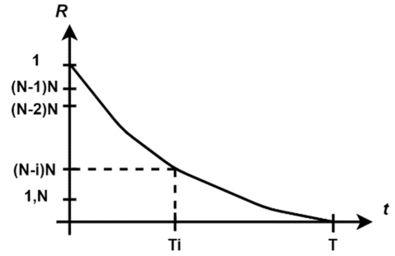
where R is the probability that the product will continue to meet the specifications, and F denotes the probability of failure, both variables being time functions, depending on the parameter t. The advantage of relation (1) is that it can be applied to systems that are fully functional or fully defective. In our context, if a chain of solar tracking systems contains irreparable products (most unfavorable scenario), the corresponding reliability curve will look like the one presented in Figure 1.

As can be seen in Figure 1, the computation of the reliability factor denoted with R relies on N products (solar tracking systems) and the final moment, denoted with T, in which all the components of the products are completely damaged.

3.1. Failure Frequency (Hazard Rate)

The failure frequency, also known as hazard rate, describes how many products are out of service (malfunctioning) in a given period. The mathematical expression associated with the failure frequency is given by Equation (2) [20]:

$$\lambda =\frac{N}{{\displaystyle \sum _{i=1}^N{T}_i}}=\frac{1}{MTF}$$

(2)

where $\lambda$ denotes the failure frequency, N the total number of products, T_i the corresponding time failures for each of the N products (industrial components), and the Mean Time to Failure (MTF) represents the average time to failure. The reliability equation will be written as in (3) [20]:

$$R_i=\frac{N-i}{N}$$

(3)

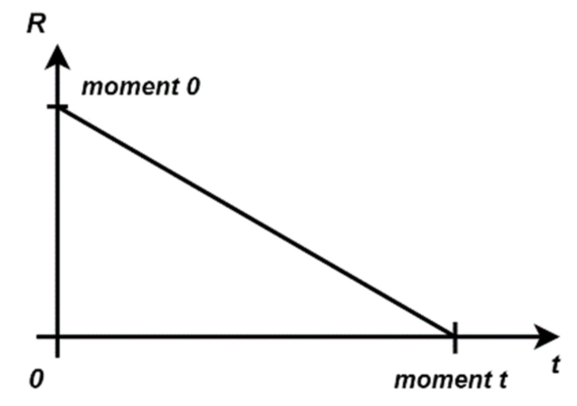
where N–i designates the number of surviving products and N the total number of products. The reliability curve diagram can be drawn accordingly as presented in Figure 2.

The derived linear reliability function can be expressed as in (4) [20]:

$$R(t)=at+b$$

(4)

where a denotes a random coordinate of the X-axis, and b denotes a random value from the Y-axis. First, according to Figure 2, the reliability linear function will be computed at moment t = 0, to determine the coordinate b, as presented in Equation (4a):

$$\begin{array}{l}R(t)=at+b=1\\ R(0)=0t+b=1\to b=1\end{array}$$

(4a)

Secondly, since we know that at t = T (final moment) the reliability will be 0, coordinate a can be computed as presented in relation (4b):

$$\begin{array}{l}R(T)=aT+b=0\\ R(T)=aT+1=0\to a=-\frac{1}{T}\end{array}$$

(4b)

According to relations (4a) and (4b), the reliability linear function can be rewritten as in Equation (5):

$$R=-\frac{t}{T}+1$$

(5)

Consider, for a more concrete case, that a test was performed on a chain of 15 PV sensors (in our case, PV cells) that are used to automate solar tracking equipment. The test time is measured in units of days. The measurement times were collected and ordered in

Table 1. Collected failure times for each of the N products.

Failure Moments (Ti)	Ti (Days)
T1	125
T2	170.83
T3	220.83
T4	283.3
T5	291.6
T6	341.6
T7	375
T8	512.5
T9	541.6
T10	583.3
T11	625
T12	666.6
T13	687.5
T14	741.6
T15	795.83

.

First, for all the collected failure times, the associated MTF and hazard rate can be determined for the solar tracker’s sensor modules. According to Equation (2), the MTF formula can be rewritten as in (6) [20]:

$$MTF=\frac{1}{N}{\displaystyle \sum _{i=1}^N{T}_i}$$

(6)

In other words, the MTF is given by the total test time divided by the total number of failures during testing phases. The MTF expression is calculated according to the catalog data from Table 1, as in expression (6a):

$$MTF=\frac{1}{N}{\displaystyle \sum _{i=1}^N{T}_i}=\frac{1}{15}(125+170.83+220.83+283.3+\dots +795.83)=$$

$$=\frac{1}{15}\cdot 6962.09=\frac{6962.09}{15}=464.1393 \mathrm{days}$$

(6a)

The corresponding failure frequency will be determined from relation (2) as seen in expression (6b):

$$\lambda =\frac{1}{MTF}=\frac{1}{464.1393}=0.0021545{ \mathrm{days}}^{-1}$$

(6b)

To establish the relative error (E) of our previous calculus, the MTF will be calculated a second time by using the following linear interpolation function of the reliability that depends on the time parameter as presented in relation (7) [20]:

$${\displaystyle \underset{0}{\overset{\infty }{\int }}R(t)\mathrm{dt}}$$

(7)

Thus, the new MTF formula will be written as in Formula (8):

$$MT{F}_1=\frac{1}{\lambda }=\frac{1}{0.0021545}=464.1393 \mathrm{days}$$

(8)

By subtracting the MTF₁ from the initial MTF relation and by dividing the result by the average time to failure, the expression (9) will be obtained as follows:

$$E=\frac{MT{F}_1-MTF}{MTF}=\frac{464.1393-464.1393}{464.1393}=\frac{0}{464.1393}=0\%$$

(9)

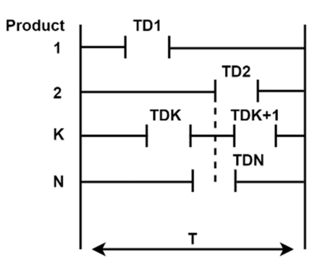
The approximation method helps determine the relative error for determining the MTF, which in our case is 0%, showing that the failure frequency calculus is accurate in establishing the time to failure model for irreparable products. For reparable components, however, failure times can be replaced by maintenance operational times which allow the fixing of damaged products, as can be seen in Figure 3.

The mathematical relation for mean downtime (MDT) will be further established, as in Equation (10) [20]:

$$MDT=\frac{1}{N_F}{\displaystyle \sum _{i=1}^{N_F}{T}_{Di}}$$

(10)

where T_Di denotes failures or maintenance times, N_F the total number of defects, and T, the total functioning time of N products. Accordantly, the operating time of the service products can be expressed as in the mathematical rule (11):

$$N\cdot T-(N_F\cdot MDT)$$

(11)

where N represents the number of components, T is the time interval, while N_F and MDT having the same meaning as in Equation (10). Consequently, at this point the Mean Time Between Failures (MTBF) formula can be defined, as in Equation (12) [21]:

$$MTBF=\frac{N\cdot T-(N_F\cdot MDT)}{N_F}$$

(12)

where the MTBF is the total operating time of all components divided by the number of occurring defects. The associated failure frequency (hazard rate) can be thus calculated with the relation (13):

$$\frac{1}{MTBF}=\frac{N_F}{N\cdot T-(N_F\cdot MDT)}$$

(13)

3.2. Availability (Efficiency)

Availability is defined as the ability of a system/equipment to be in working order under given conditions, at a given time, or for a given period, assuming that the provision of the necessary external means (maintenance) is ensured [13]. Availability is considered a complex form of assessing the quality of a system/product because it includes both reliability and maintainability. Mathematically, availability can be expressed as in Equation (14) [20]:

$$A=\frac{N\cdot T-N_F\cdot MDT}{N\cdot T}$$

(14)

Based on Equation (12) the formula for the product N$\cdot$T can be rewritten as in relation (15):

$$N\cdot T=N_F\cdot MTBF+N_F\cdot MDT$$

(15)

According to Equation (15) we can now write the final form of A from (14):

$$A=\frac{MTBF}{MTBF+MDT}$$

(16)

where, for convenience, the MTF and MTBF parameters can be used to characterize the automated system. In conclusion, a product or component is available as long as it can provide service, and unavailable when it is undergoing maintenance operations. As seen in Equation (1), the probability model of availability and unavailability can be expressed as in the mathematical rule (17) [20]:

$$A+U=1\to U=1-A$$

(17)

More generally, we will write unavailability as in the Equation (18):

$$U=\frac{MDT}{MTBF+MDT}$$

(18)

where unavailability depends only on the MDT divided by the total time (operating time + malfunctioning time). Consider, for a real-life scenario, that a company acquires 30 identical motor drivers that are used in solar tracking systems and perform a test on them for 3 months, recording the failure times (maintenance times), measured in days, in

Table 2. Malfunctioning (Repairing Service Times) Collected During 3 Months (expressed in days units).

Batches (B)	B1	B2	B3	B4	B5	B6	B7	B8
Maintenance Operation Days	2	4	3	2	7	4	1	6
	3	2	4	3	8	6	5	5
	1	5	1	5	1	1	2	1
	5	1	1	4	3	2	3	2
	6	7	2	1	2	1	4	3

.

According to Table 2, the active number of failures is N_F = 40. The total time is calculated for N_T = 30 $\cdot$90 $\cdot$24 = 64800 h = 2700 days. Accordingly, we can compute the MDT parameter with the relation (19):

$$\begin{array}{l}MDT=\frac{1}{N_F}{\displaystyle \sum _{i=1}^{N_F}{T}_{Di}}=\frac{1}{40}(2+3+1+5+6+\dots +3)=\\ =\frac{1}{40}\cdot 129=3.225 \mathrm{days}\end{array}$$

(19)

The total failure time will then be calculated with the Formula (20):

$$N_F\cdot MDT=40\cdot 3.225=129 \mathrm{days}$$

(20)

Furthermore, the MTBF will be determined with relation (21):

$$\begin{array}{l}MTBF=\frac{N\cdot T-(N_F\cdot MDT)}{N_F}=\frac{30\cdot 90-129}{129}=\\ =\frac{2700-129}{129}=\frac{2571}{129}=19.93 \mathrm{days}\end{array}$$

(21)

The failure frequency will be computed with Equation (22):

$$\begin{array}{l}\lambda =\frac{1}{MTBF}=\frac{N_F}{N\cdot T-(N_F\cdot MDT)}=\frac{129}{30\cdot 90-129}=\\ \frac{129}{2700-129}=\frac{129}{2671}=0.05\end{array}$$

(22)

At this point the availability and unavailability parameters (Equations (16), (17), and (18)) can be established based on the previously calculated values with Formula (23):

$$\begin{array}{l}A=\frac{MTBF}{MTBF+MDT}=\frac{19.9}{19.9+3.225}=\frac{19.9}{23.125}=0.86\\ U=\frac{MDT}{MTBF+MDT}=\frac{3.225}{19.9+3.225}=\frac{3.255}{20.925}=0.14\\ A+U=0.86+0.14=1\end{array}$$

(23)

By relying on the previous standard metrics, the general conclusion is that the MTBF is 19.9 days and the MTF is 3.225 days, which means that once every approximately 19 days one motor driver malfunctions and requires 3.225 days for maintenance operations, resulting in an 86% availability rating and 14% unavailability rating.

3.3. Typical Variation Form of the Hazard Rate (Bathtub Curve)

The variation in time of the reliability function (R) in regards to the hazard rate ($\lambda$) can be expressed mathematically as in Equation (24) [21]:

$$\frac{dR}{R}=-\lambda (t)dt$$

(24)

It was already stated that at moment t = 0 all the products function according to their operating specifications so that the relationship between reliability and the instantaneous failure rate is established with the help of the equation system (25) [21]:

$$\left\{\begin{array}{l}R(\mathrm{t})={\mathrm{e}}^{-{\displaystyle \underset{0}{\overset{t}{\int }}\lambda (t)dt}}\\ \lambda =ct\end{array}\right.\to R(\mathrm{t})={\mathrm{e}}^{-\lambda {\displaystyle \underset{0}{\overset{t}{\int }}dt}}=e^{-\lambda t}$$

(25)

Generally, the MTF relation will become as presented in (26):

$$\left\{\begin{array}{l}\Delta F(t)=R(t)+F(t)\\ F(t)=1-e^{-\lambda t}\end{array}\right.\to MTF=\frac{1}{\lambda }$$

(26)

The MTF Formula (27) is given consequently by the subgraph area:

$$MTF={\displaystyle \underset{0}{\overset{\infty }{\int }}R(t)dt=\frac{1}{\lambda }}$$

(27)

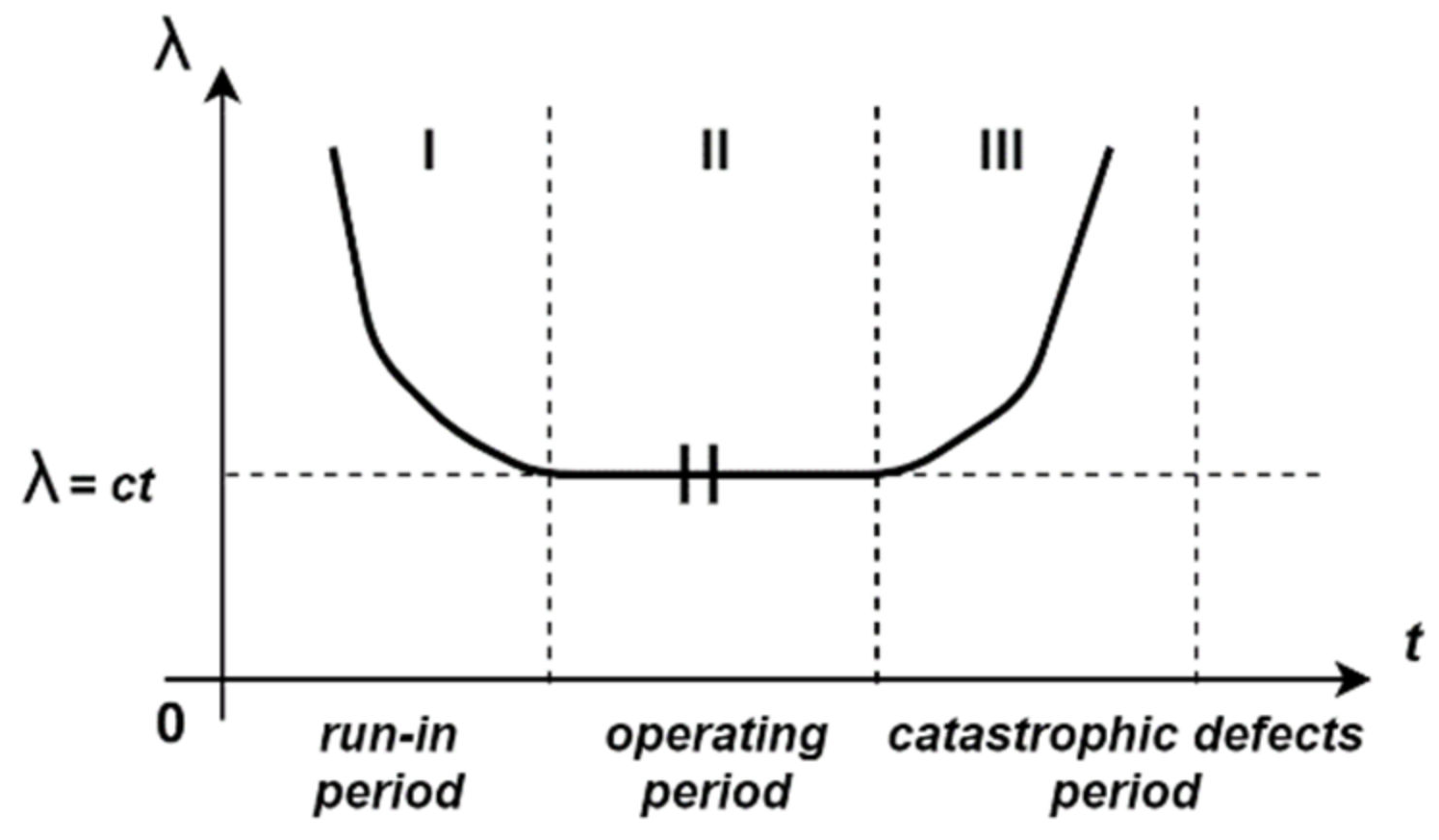
The graphical representation of Equation (26) can be seen in Figure 4.

This graphical representation applies to any solar tracking system (automation equipment) which is described by the run-in period (usually around 6 months) followed by the normal operating period (warranty period, which depends on the quality of the acquired product) and, lastly, the catastrophic defect area where generally, a solar tracking system will require several maintenance human interventions.

Finally, there is a second and last approach for analyzing the typical variation form of the hazard rate, given by the so-called Weibull distribution model, found in relation (28) [21]:

$$\lambda (t)=\frac{\beta }{\eta }{(\frac{t-t_0}{\eta })}^{\beta -1},\beta >0$$

(28)

According to Equation (28), the relation for the reliability variation can be written in the Equation (29):

$$R(t)=\exp \left[-{(\frac{t-t_0}{\eta })}^{\beta }\right]$$

(29)

where β is a positional parameter, η is a scalar parameter, t₀ is the initial moment, and exp represents the exponential form of Euler’s constant named value.

3.4. Applications

The abovementioned metrics can be applied to a variety of real-life scenarios regarding the calculus of reliability, MTF, MDT, and hazard rate of solar tracking systems. More specifically, to establish accurate predictions about the reliability of the entire solar tracking system, it is of major importance to formulate problems concerning the failure rates of a solar tracker’s components. For instance, consider that an MCU (e.g., Arduino UNO) which is used to control solar tracking equipment, has a constant failure rate of 0.1 / year, and we want to determine the reliability, respectively the probability of failure for 1, 2, and 3 years. This problem can be solved by just relying on the equation set (30) as follows:

$$\left\{\begin{array}{l}R(t)=e^{-{\displaystyle \underset{0}{\overset{t}{\int }}\lambda (t)dt}}\\ R(t)=e^{-\lambda t}\\ R(1year)=e^{-0.1\times 1}=e^{-0.1}=0.9048=90.48\%\\ F(1year)=1-R(year)=0.0952=9.52\%\\ R(2years)=e^{-0.1\times 2}=e^{-0.2}=0.8187=81.87\%\\ F(2years)=1-R(2years)=0.1813=18.13\%\\ R(3years)=e^{-0.1\times 3}=e^{-0.3}=0.7408=74.08\%\\ F(3years)=1-R(3years)=0.2592=25.92\%\end{array}\right.$$

(30)

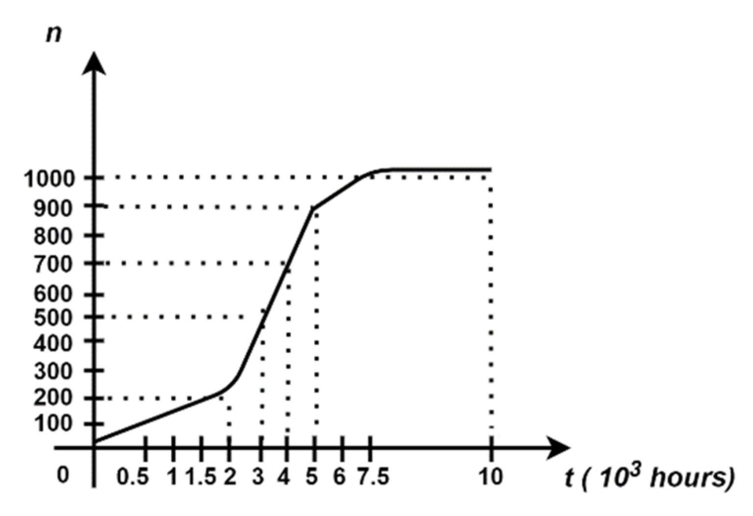
The aforementioned solution shows that the reliability of the Arduino UNO board decreases in years by an average value of 8%, while the chance of failure increases every year by approximately 9%. Another way to analyze the behavior of solar tracking systems is from the defects points of view, according to a Weibull distribution given by the parameters t₀ = 0, η = 625 days and β = 1.5. It is considered that for the given input parameters, a test was performed on 1000 random components that were mass-produced to construct solar trackers. The goal here is to determine the survival (operating) probability of these components after t = 10⁴ h, by applying the Weibull equation, as presented in (31):

$$\begin{array}{l}R(t)=\exp \left[-{(\frac{t-t_0}{\eta })}^{\beta }\right]=\exp \left[-{(\frac{416.6-0}{625})}^{1.5}\right]=\exp \left[-{(\frac{416.6}{625})}^{1.5}\right]=\\ =\exp (-0.5442)=0.5803=58.03\%\end{array}$$

(31)

Additionally, for another queue of 1000 random components that were mass-produced in the industrial environment, it is of interest to determine the period after which 100 components became faulty. It is assumed that the component testing was started at the moment t = 0. Therefore, if t₀ = 1000 components, moment t₁ will correspond to the subtraction of 100 components from the initial stack, in other words, t₁ = 1000 – 100 = 900 remaining components. The associated reliability R(t₀) = 1 (as a general rule) and R(t₁) = 0.9. The expression of R(t₁) is expanded according to Formula (32):

$$\begin{array}{l}R(t_1)=\exp \left[-{(\frac{t_1-t_0}{\eta })}^{\beta }\right]\\ \ln R(t_1)=\ln \left[\exp \left[-{(\frac{t_1-t_0}{\eta })}^{\beta }\right]\right]\to \ln R(t_1)=-{(\frac{t_1-t_0}{\eta })}^{\beta }\\ \ln \frac{1}{R(t_1)}={(\frac{t_1-t_0}{\eta })}^{\beta }\to \ln \ln \frac{1}{R(t_1)}=\beta \cdot \ln (t_1-t_0)-\beta \cdot \ln \eta \\ \to \ln (t_1-t_0)=(\ln \ln \frac{1}{R(t_1)}+\beta \cdot \ln \eta )\cdot \frac{1}{\beta }\end{array}$$

(32)

Following, the last obtained expression for t₀ = 0 will be computed as in (33):

$$\begin{array}{l}{t}_1=e^{\frac{1}{\beta }(\ln \ln \frac{1}{R(t_1)}+\beta \ln \eta )}\to t_1=e^{\frac{1}{1.5}(\ln \ln \frac{1}{0.9}+1.5\ln 1.5\cdot {10}^4)}\to \\ \to t_1=e^{\frac{1}{1.5}(-2.25+9.6158)}\to t_1=0.38170987 \mathrm{years}\end{array}$$

(33)

Finally, a more convenient manner to represent the number of faulty components is through a graph chart which shows the evolution in time of 10 pairs containing 100 components each, until the final moment where all products are completely damaged, as can be seen in Figure 5.

4. Proposed Fault Coverage-Aware Model for Calculating the Solar Reliability Factor

Since the standard Weibull method relies initially on the computation of time to failure models such as MTF, MDT, and MTBF which are usually applied to individual components, this paper proposes a set of three fault coverage-aware metrics that make use of experimental data gathered from hardware, software and in-circuit oriented testing techniques.

The aim of testing electronic solar tracking equipment is to identify errors that may occur in digital circuits. Reliability analysis is crucial for businesses as well as regular consumers for choosing robust and long-lasting components. To satisfy these needs, the reliability of solar trackers is calculated in two major ways: (a) by using hardware testing equipment such as built-in self-test (BIST) modules and (b) by focusing on the calculus of reliability based on white-box software testing (WBST) algorithms.

4.1. Fault-Coverage Aware Metric for Determining the Reliability of Electronic Components with the Help of BIST Devices

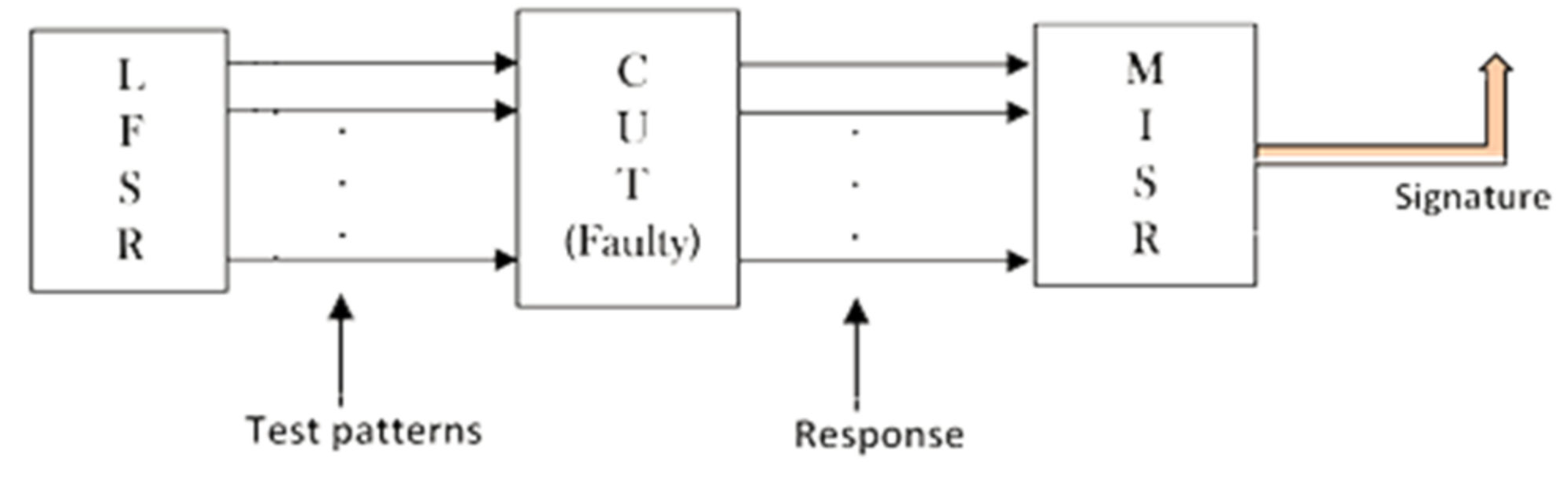
BIST architectures are today’s preferred hardware testing routines due to their facile deployment and integration in various digital circuits, thus eliminating the need of employing standalone automated test equipment (ATE). A static deployed BIST architecture is generally composed of three components: (a) test pattern generator (TPG) which injects test vectors into the circuit chain, (b) device under test (DUT), sometimes also referred to as circuit under test (CUT), and (c) output response analyzer (ORA) which collects the outputted signals of the CUT and generates corresponding signatures for each of the patterns, as can be seen in Figure 6.

Usually, a BIST architecture makes use of a linear feedback shift register (LFSR) as a TPG unit and a multiple input signature register (MISR) as an ORA unit, both hardware devices relying on the deployment of D-type flip flops (FFs). More important, however, is the fact that the total number of deployed FFs in the MISR unit increases the chance of detecting hardware errors, implicitly expanding the fault coverage domain. Therefore, during the BIST routine’s testing phase, collected data (signatures) from the experimental cases is used to outline the fault coverage. Further, an STF parameter is defined, which will be expressed mathematically as in Formula (34):

$$STF=\frac{N_E\cdot T_V}{T_P\cdot 2^D}$$

(34)

where T_V represents the number of executed test vectors, N_E the number of errors per test case, T_P the total number of test patterns, and D the number of identical devices used for detecting errors (which in our case are given by the FF units). Since the generalized STF formula can be adapted to various test scenarios, several STF properties will be listed as follows:

(1)

The number of errors N_E is always equal, lower, or greater than T_V in any test scenario regardless of the noise factors that are considered, and can be expressed mathematically as in (35):

$$N_E\ge T_V\_\_N_E\le T_V\_\_N_E,T_V\in \mathbb{N}$$

(35)

(2)

The number of test vectors T_V is always equal to or lower than the total number of test patterns T_P given by the expression (36):

$$T_V\le T_P\_\_T_V,T_P\in \mathbb{N}$$

(36)

(3)

The total number of test patterns is calculated with the Equation (37):

$$T_P=2^D-1$$

(37)

(4)

If no errors are detected during the testing routines, the STF parameter will be 0 resulting in 100% reliability and availability of the tested equipment, expressed in Equation (38):

$$STF=0\leftrightarrow R=A=1$$

(38)

To demonstrate the validity of these properties, a few concrete cases are presented further. Regarding the STF, the following considerations are listed: (a) for a total number of T_V = 7 (test cases) the test system has successfully identified N_E = 10 bit-flip errors. It should be noted, according to property (1) that the number of errors detected may be greater than the number of test cases because multiple errors (burst errors) may occur within a single test vector. Additionally, for (b) a number D = 4 FFs are used in the structure of the MISR in this paper. According to property (3), the total number of test cases T_P is calculated based on the Formula (39):

$$T_P=2^D-1\to T_P=2^4-1=15$$

(39)

Since T_V = 7 and T_P = 10 property (2) is also satisfied. Finally, by having this hypothetical data the variables from Equation (34) can be adequately substituted as in (40):

$$STF=\frac{10\cdot 7}{15\cdot 16}=\frac{70}{240}=0.29\approx {0.30}_{ }$$

(40)

Supposing that during the detection stage, all the errors were corrected by using the Hamming code algorithms, parameter N_E will be reduced to the value 0. The corresponding equation will be expressed as in (41):

$$STF=\frac{0\cdot 7}{15\cdot 16}=\frac{0}{240}=0\to R=A=1$$

(41)

thus satisfying property (4) of the first set of metrics. In the last stage the SRF will be calculated with the Formula (42):

$$SRF=\exp [\frac{N_E\cdot T_V}{T_P\cdot 2^D}]$$

(42)

Since the SRF expression is the exponential of the STF equation, the entire relationship can be rewritten as in expression (43):

$$SRF=e^{-STF}$$

(43)

At this point, the SRF of the automated sun-tracking equipment will be computed as in Equation (44):

$$SRF=e^{-STF}=e^{-0.3}=\frac{1}{e^{0.3}}=\frac{1}{{2.71}^{0,3}}=\frac{1}{1.3486}=0.74$$

(44)

Similarly, if the STF parameter is reduced to 0, the mathematical expression will become as in expression (45):

$$SRF=e^{-STF}=e^{-0}=\frac{1}{e^0}=\frac{1}{1}=1\leftrightarrow R=A=1$$

(45)

The final mathematical relation connects the SRF parameter with the initially computed STF variable according to property (4), thus showing that hardware components that are not affected by permanent errors can achieve 100% reliability and availability. Any other types of defects caused by transient errors can be considered negligible since their footprint on the electronic components is only temporary and does not cause any serious harm to the overall functionality of the tested devices [6].

4.2. Fault-Coverage Aware Metric for Determining the Reliability of Electronic Components with the Help of WBST Methods

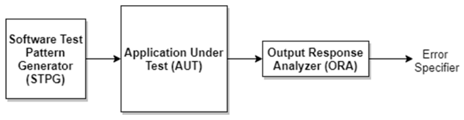
Traditional testing processes aim to generate test vector sets that apply to a specific fault model to optimize coverage while reducing the execution time of the test application. Because the Off-Line test is typically performed after the circuit is assembled as part of a more in-depth manufacturing test, it is often used in maintenance checking for extending the lifespan of the product. Roughly equivalent to off-line testing, on-line testing, also referred to as parallel or concurrent error detection, is a test technique used to permanently verify the integrity of the CUT, as can be seen in Figure 7. One of the preferred on-line software testing techniques is known under the acronym of WBST routines which periodically checks the CUT for transient or permanent errors. A more particular case of the WBST method is the cloud-based software testing technique which makes use of an Internet of Things (IoT) software TPG for injecting test vectors in MCU devices which are part of solar tracking equipment.

By stimulating the inputs of the CUT the outputs are collected in a results gatherer where with the help of an error indicator, the user is capable to establish the fault coverage of the employed WBST method. Moreover, as expected, the previous metric set presented in Section 4.1 for our software test scenarios can be adapted adequately. The STF formula corresponding to the WBST routines will be written as in Equation (46):

$$STF=\frac{N_E\cdot T_V}{T_P\cdot 2^B}$$

(46)

where N_E represents the number of errors per test vector, T_V denotes the number of considered test vectors, T_P provides the total number of test patterns and B designates the number of breakpoints/software functions that are implemented across the algorithm debugging stage.

Besides this minor difference from the proposed hardware metric, a few other properties which are important for demonstrating the validity of the software-based metric will be listed below:

(1)

The number of errors N_E is always equal, lower, or greater than T_V in any test scenario regardless of the number of considered breakpoints, and can be expressed mathematically as in statement (47):

$$N_E\ge T_V\_\_N_E\le T_V\_\_N_E,T_V\in \mathbb{N}$$

(47)

(2)

The number of test vectors T_V is always equal to or lower than the total number of test patterns T_P given by the expression (48):

$$T_V\le T_P\_\_T_V,T_P\in \mathbb{N}$$

(48)

(3)

If no errors are detected during the testing routines the STF parameter will be 0 resulting in 100% reliability and availability of the tested equipment, expressed as in Equation (49):

$$STF=0\leftrightarrow R=A=1$$

(49)

As already anticipated, the second metric removes one of the listed properties from Section 4.1 since there is no clear mathematical relationship between the total number of test patterns T_P and the number of breakpoints B. At this point, the validity of the remaining three properties can be demonstrated in a real-life scenario. Regarding the STF, the following considerations are made: (a) for a total number T_V = 7 (test cases), the test system has successfully identified N_E = 10 calculation errors. Additionally, for (b) a number of T_P = 10 test patterns and a number B = 10 breakpoints in the software code, meaning that the test system successfully identified all calculation errors with the deployed software functions. Because properties (1) and (2) are already satisfied from the above statement, let the STF parameter will be calculated as in relation (50):

$$STF=\frac{10\cdot 7}{10\cdot 10}=\frac{70}{100}=0.70$$

(50)

In the last stage, the SRF parameter will be computed with the mathematical rule (51):

$$\begin{array}{l}SRF=\exp [\frac{N_E\cdot T_V}{T_P\cdot 2^D}]=e^{-STF}=e^{-0.7}=\frac{1}{e^{0.7}}=\frac{1}{{2.71}^{0.7}}=\\ =\frac{1}{2}=0.50\end{array}$$

(51)

showing that with almost the same hypothetical set of data from Section 4.1, the reliability of the solar tracking equipment is halved. This is because calculation errors in the software code usually manifest in the behavioral model of the hardware device (incoherent stepper motor rotations leading to improper positioning of the solar panel thus resulting in heavy energy harvesting losses). Along with the satisfying property (3) of the second set of metrics, consider that during the detection stage all the errors were manually corrected by the software engineer, thus minimizing NE to the value 0. The final Equation (52) will become:

$$SRF=e^{-STF}=e^{-0}=\frac{1}{e^0}=\frac{1}{1}=1\leftrightarrow R=A=1$$

(52)

4.3. Fault-Coverage Aware Metric for Determining the Reliability of Electronic Components with the Help of ICT Methods

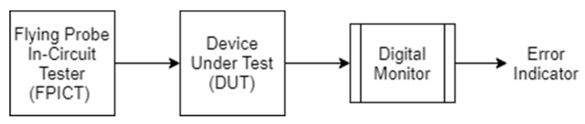
ICT is a type of white-box testing procedure where an electrical probe navigates the entire printed circuit board (PCB) area to identify shorts, opens, resistance, capacitance, and other basic electrical components which give a hint of the electronic assembly which was fabricated according to its catalog specifications [8]. The ICT process is conducted with the help of industrial machines such as ATE, bed of nails fixtures, or with a fixtureless ICT setup (one example here being a flying probe device). In work [8], a flying probe inspired in-circuit tester (FPICT) was constructed and deployed to verify the integrity of the entire solar tracking electrical equipment. By implementing a sensorless solution for locating all test points of the PCB, the proposed test device was capable to monitor critical paths and parameters (such as current and voltage drops), thus determining a fault coverage of the malfunctioning CUTs, as can be seen in Figure 8.

To demonstrate the flexibility of the metrics set, the mathematical expressions from Section 4.1 and Section 4.2 will be adapted to the ICT test scenarios. The STF formula corresponding to the ICT routines will be written as in expression (53):

$$STF=\frac{N_E\cdot T_R}{N_R\cdot 2^P}$$

(53)

where N_E represents the number of errors per test round, T_R denotes the number of considered test rounds, N_R provides the total number of test routines and P designates the number of probes (nails) that are equipped to the FPICT device.

Similarly, as in the previous sections, the properties which are essential for validating the ICT-based metric will be listed below:

(1)

The number of errors N_E is always equal, lower, or greater than T_R in any test scenario regardless of the number of probes that are used during testing, and can be expressed mathematically as in expression (54):

$$N_E\ge T_R\_\_N_E\le T_R\_\_N_E,T_R\in \mathbb{N}$$

(54)

(2)

The number of test rounds T_R is always equal to or lower than the total number of test routines N_R, given by the expression (55):

$$T_R\le N_R\_\_T_R,N_R\in \mathbb{N}$$

(55)

(3)

If no errors are detected during the testing routines the STF parameter will be 0 resulting in 100% reliability and availability of the tested equipment, expressed as in relation (56):

$$STF=0\leftrightarrow R=A=1$$

(56)

Consider a real-life scenario where all possible test points’ voltage deviations must be identified. For this purpose, the test system implements a number of T_R= 10 rounds for each test point, a total number of N_R = 100 test routines, and a number of P = 2 probes, to identify N_E = 12 voltage deviations. The STF parameter will be computed in relation (57), based on the previous configuration:

$$STF=\frac{N_E\cdot T_R}{N_R\cdot 2^P}=\frac{12\cdot 10}{100\cdot 2^2}=\frac{120}{400}=0.30$$

(57)

With the abovementioned result properties (1) and (2) are successfully satisfied. To demonstrate property (3), a similar but fault-free DUT is considered, leading to the Formula (58):

$$STF=\frac{N_E\cdot T_R}{N_R\cdot 2^P}=\frac{0\cdot 10}{100\cdot 2^2}=\frac{0}{400}=0\leftrightarrow R=A=1$$

(58)

The SRF parameter will be calculated as in Equations (59) and (60):

$$SRF=e^{-STF}=e^{-0.3}=\frac{1}{e^{0.3}}=\frac{1}{{2.71}^{0.3}}=\frac{1}{1.3486}=0.74$$

(59)

$$SRF=e^{-STF}=e^{-0}=\frac{1}{e^0}=\frac{1}{1}=1\leftrightarrow R=A=1$$

(60)

The above described metrics reduce significantly the number of computations executed during the Weibull distribution algorithm, as well as the number of parameters that are involved in the mathematical rules, proving that fault coverage is a promising reliability and availability indicator.

5. Experimental Setup and Results

This section presents the experimental setup and results as well as a comparison between our work and other related manuscripts from the targeted domain.

5.1. Fault Coverage-Aware Metrics Equation Reduction for Computing the Reliability Test Factor

With regards to our simulation setup, the experimental data is obtained from works [6,7,8], to outline the efficiency and fast computation of the previously described hardware and software fault coverage-aware metrics. Before describing the experimental environment the number of parameters in each equation is narrowed down, to adapt the metrics to the BIST and WBST test scenarios.

First, according to Equation (34) for the BIST routines, it was established that the STF parameter is directly proportional to the number of test vectors multiplied by the number of errors (per test vector) and inversely proportional to the total number of test patterns multiplied by 2 to the power of D (where D denotes the number of FFs devices used during the testing stage). At this point, Equation (34) will be constrained by the properties mentioned in Section 4, a reason for which the product N_E $\cdot$ T_V will be denoted with E, representing the hardware error factor. According to property (3), Equation (34) can be rewritten as in relation (61):

$$STF=\frac{E}{2^D\cdot (2^D-1)}$$

(61)

Secondly, by knowing the STF parameter for the WBST routines, the following associations can be realized similarly as in Equation (62):

$$STF=\frac{E}{T_P\cdot 2^B}$$

(62)

where E designates the error factor for software testing, T_P the number of software test patterns, and B the number of breakpoints used during the debugging stage.

Finally, by adapting the STF parameter for the ICT routines, the formula can be simplified as in relation (63):

$$STF=\frac{E}{N_R\cdot 2^P}$$

(63)

where E represents the error factor for ICT, N_R the total number of test routines, and P the total number of test probes. Thus, by reducing the equations to the simplest form, we can proceed with the description of the simulation environment and the reliability graph generation of the tested solar tracking system.

5.2. Fault Coverage-Aware Metrics for BIST, WBST, and ICT Test Scenarios

Based on our previous efforts to verify the functionality of the solar tracking equipment described in [6,7,8], we can further use the collected experimental data to validate the proposed fault coverage-aware metrics. Since BIST-oriented architectures and WBST algorithms are applied to check various digital devices involved in the automation process of the solar tracking device, the results will be organized similarly to the Weibull distribution model. Even though the experimental results were gathered only from a personalized solar tracking prototype, we firmly sustain the idea that the proposed fault coverage-aware metrics can be generalized for several solar tracking systems available on the market today. Regarding the experimental data obtained from the online built-in self-test (OBIST) architecture presented in [7], the total number of test patterns and detected errors are synthesized in

Table 3. Extended Fault Analysis of Single Bit-Flip Errors As Well As Single Stuck-At-Faults [7].

Crt. No.	Initial Seed (HEX)	Fault Coverage		Total Test Patterns	Total Detected Errors
		Single Bit Flip Errors	Single Stuck-at-Faults
		Last 8 Bits (Mutant)
1	FFFF	93.95%	100 %	65,535	61,570
2	8FFF	93.93%			61,557
3	8CFF	93.92%			61,550
4	8C9F	93.91%			61,544
5	8C94	93.94%			61,563

.

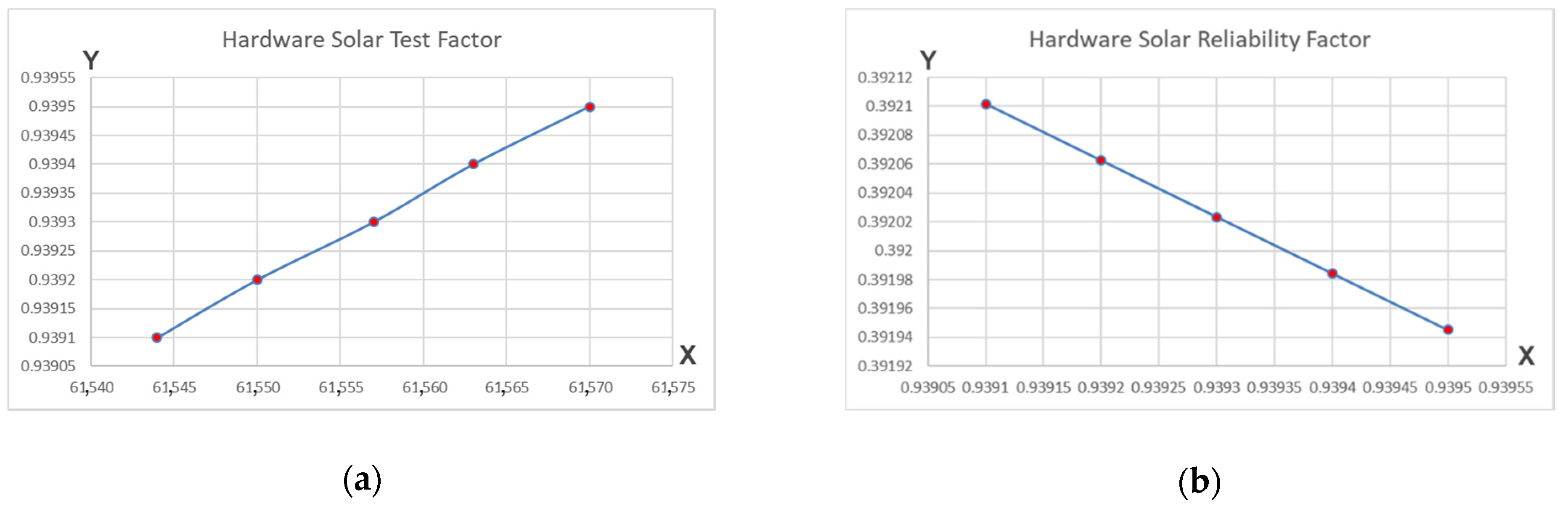
According to the data in Table 3, it can be observed that the total number of patterns T_P is a constant value (see column 5) and the error factor E is a variable parameter (see column 6). Thus, to generate the graphical representation of the STF parameter, the following equation system (64) must be computed:

$$\left\{\begin{array}{l}STF=\frac{E}{2^D\cdot (2^D-1)}\\ T_P=2^D-1\\ STF(E_1)=\frac{E_1}{2^D\cdot (2^D-1)}\\ STF(E_2)=\frac{E_2}{2^D\cdot (2^D-1)}\\ STF(E_3)=\frac{E_3}{2^D\cdot (2^D-1)}\\ STF(E_4)=\frac{E_4}{2^D\cdot (2^D-1)}\\ STF(E_5)=\frac{E_5}{2^D\cdot (2^D-1)}\end{array}\right.$$

(64)

where D is also a constant value that comprises 16 FFs units involved in the OBIST routines. Therefore, the following results are presented in the equation system (65):

$$\left\{\begin{array}{l}STF=\frac{E}{2^{16}\cdot (2^{16}-1)}\\ T_P=2^{16}-1\\ STF(E_1)=\frac{61,570\cdot 65,535}{2^{16}\cdot (2^{16}-1)}=\frac{61,570}{65,534}=0.9395\\ STF(E_2)=\frac{61,557\cdot 65,535}{2^{16}\cdot (2^{16}-1)}=\frac{61,557}{65,534}=0.9393\\ STF(E_3)=\frac{61,550\cdot 65,535}{2^{16}\cdot (2^{16}-1)}=\frac{61,550}{65,534}=0.9392\\ STF(E_4)=\frac{61,554\cdot 65,535}{2^{16}\cdot (2^{16}-1)}=\frac{61,544}{65,534}=0.9391\\ STF(E_5)=\frac{61,563\cdot 65,535}{2^{16}\cdot (2^{16}-1)}=\frac{61,563}{65,534}=0.9394\end{array}\right.$$

(65)

After computing the equation set (65), it can be immediately noticed that the STF parameter is tightly coupled to the fault coverage (FC) domain in Table 3 (see column 3). In other words, the mathematical relation between the two parameters can be written as seen in Formula (66):

$$STF=\frac{FC}{100}\leftrightarrow FC=STF\cdot 100$$

(66)

The abovementioned equation proves that the defined STF parameter is the fault coverage percentage written in fractional form. By ordering the results in the equation set (64), the graphical representation of the STF factor will be obtained in form of a linear function, as can be seen in Figure 9 (scenario a). As expected, the more errors are detected utilizing hardware testing techniques (OBIST in our case), the more the STF linear function will increase, according to the fault coverage principle.

Following, the SRF parameter can be computed according to the equation set in (67) where STF₁, STF₂, STF₃, STF_4, and STF₅ were previously calculated in the equation set (64).

$$\left\{\begin{array}{l}SRF=e^{-STF}=\frac{1}{e^{STF}}\\ SRF(ST{F}_1)=e^{-ST{F}_1}=\frac{1}{e^{ST{F}_1}}=0.3919\\ SRF(ST{F}_2)=e^{-ST{F}_2}=\frac{1}{e^{ST{F}_2}}=0.3920\\ SRF(ST{F}_3)=e^{-ST{F}_3}=\frac{1}{e^{ST{F}_3}}=0.3920\\ SRF(ST{F}_4)=e^{-ST{F}_4}=\frac{1}{e^{ST{F}_4}}=0.3921\\ SRF(ST{F}_5)=e^{-STF5}=\frac{1}{e^{ST{F}_5}}=0.3919\end{array}\right.$$

(67)

Thus, the graphical representation is a linear function that describes the reliability factor of the entire solar tracking system, as shown in Figure 9 (scenario b).

All the presented results were simulated and computed in the Mathcad v15 environment due to its extensive and facile engineering tools.

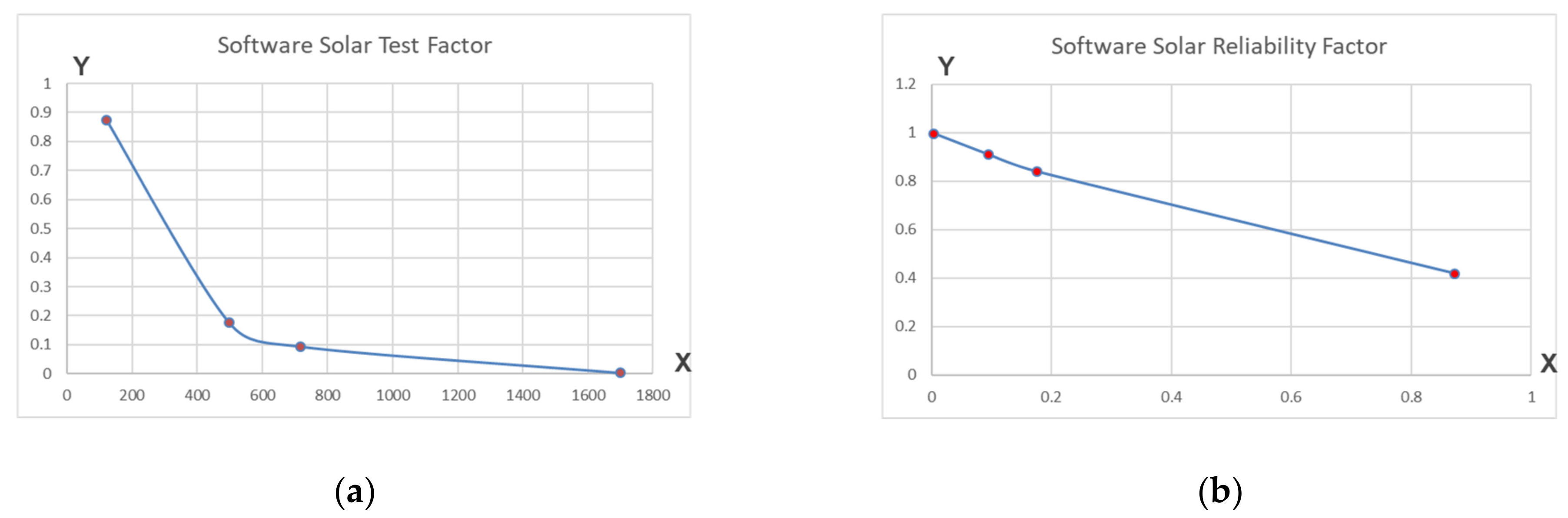
Furthermore, it was determined that the granularity of each graphical representation can be controlled by adding more test case scenarios to the fault coverage database. Similarly, with regards to the On-line WBST presented in [6], the experimental results in

Table 4. WBST Fault Coverage for Control Flow, Communication, Calculation, and Error Handling Errors [6].

Crt. No.	Total Detected Errors				Total Test Patterns	Error Coverage (%)
	Control Flow Errors	Communication Errors	Calculation Errors	Error Handling Faults
1	395	2	568	736	2277	74.70
2	175	1	242	299	1087	65.96
3	118	1	166	214	840	59.40
4	78	0	2	42	130	93.84

were synthesized according to four test batches which contain a huge amount of data packets.

For each of the listed data batches depicted in Table 4, we associated a number of 10 breakpoints/software functions that are distributed along with the algorithm to detect as many error types as possible.

Here, it can be observed that the total number of test patterns is T_P = 4334 (computed by adding all test vectors together from column 6), and the variable number of errors E is calculated for each data batch. By using the simplified Equation (62), the equation set for calculating the STF parameter in regards to the WBST routines will be constructed as in equation system (68):

$$\left\{\begin{array}{l}STF=\frac{E}{T_P\cdot 2^B}\\ STF(E_1)=\frac{E_1}{T_P\cdot 2^B}=\frac{1701\cdot 2277}{4334\cdot 1024}=\frac{3,873,177}{4,438,016}=0.8727\\ STF(E_2)=\frac{E_2}{T_P\cdot 2^B}=\frac{717\cdot 1087}{4334\cdot 1024}=\frac{779,379}{4,438,016}=0.1756\\ STF(E_3)=\frac{E_3}{T_P\cdot 2^B}=\frac{499\cdot 840}{4334\cdot 1024}=\frac{419,160}{4,438,016}=0.0944\\ STF(E_4)=\frac{E_4}{T_P\cdot 2^B}=\frac{122\cdot 130}{4334\cdot 1024}=\frac{15,860}{4,438,016}=0.0035\end{array}\right.$$

(68)

By solving the equation set (68), it can be immediately noticed that the STF parameter for software test scenarios is completely different from the FC (see column 7). Therefore, the graphical representation of the STF for WBST routines is a curve distribution, as can be seen in Figure 10 (scenario a).

Finally, the equation set (69) for the SRF parameter can be computed accordantly:

$$\left\{\begin{array}{l}SRF=e^{-STF}=\frac{1}{e^{STF}}\\ SRF(ST{F}_1)=e^{-ST{F}_1}=\frac{1}{e^{ST{F}_1}}=0.9965\\ SRF(ST{F}_2)=e^{-ST{F}_2}=\frac{1}{e^{ST{F}_2}}=0.9101\\ SRF(ST{F}_3)=e^{-ST{F}_3}=\frac{1}{e^{ST{F}_3}}=0.8394\\ SRF(ST{F}_4)=e^{-ST{F}_4}=\frac{1}{e^{ST{F}_4}}=0.4189\end{array}\right.$$

(69)

As can be seen in Figure 10 (scenario b), the graphical representation of the STF parameter is a linear distribution and proves that improved fault coverage results in high reliability because software errors can be corrected manually by the software engineer, in comparison to hardware faults which require in certain scenarios the total replacement of the components. Finally, by extending the test scenarios for the FPICT method [8], the experimental dataset presented in

Table 5. Extended ICT Fault Coverage for Multiple Point Testing Results [8].

Crt. No.	Test Type	No. of Test Samples (Parameters)	Fault Coverage (%)
1	Multiple Point Testing	250	88.70
2			90
3			91.40
4			95.70

will be obtained.

According to the four multiple point testing batches seen in Table 5, the error factor E can be determined based on the equation set (70):

$$\left\{\begin{array}{l}E=T_R\cdot FC\\ E_1=T_R\cdot F{C}_1\to E_1=250\cdot \frac{88.70}{100}=221.75\\ E_2=T_R\cdot F{C}_2\to E_2=250\cdot \frac{90}{100}=225\\ E_3=T_R\cdot F{C}_3\to E_3=250\cdot \frac{91.40}{100}=228.5\\ E_4=T_R\cdot F{C}_4\to E_4=250\cdot \frac{95.70}{100}=239.25\end{array}\right.$$

(70)

where T_R is a constant value (see column 3) and FC is the variable fault coverage determined for each test batch (see column 4). Following, the calculated values from the equation system (70) will be substituted in the STF equation set (71):

$$\left\{\begin{array}{l}STF=\frac{E}{N_R\cdot 2^P}\\ STF(E_1)=\frac{E_1}{N_R\cdot 2^P}=\frac{221.75}{1000\cdot 2}=\frac{221.75}{2000}=0.1108\\ STF(E_2)=\frac{E_2}{N_R\cdot 2^P}=\frac{225}{1000\cdot 2}=\frac{225}{2000}=0.1125\\ STF(E_3)=\frac{E_3}{N_R\cdot 2^P}=\frac{228.5}{1000\cdot 2}=\frac{228.5}{2000}=0.1142\\ STF(E_4)=\frac{E_4}{N_R\cdot 2^P}=\frac{239.25}{1000\cdot 2}=\frac{239.25}{2000}=0.1196\end{array}\right.$$

(71)

Finally, after solving the equation set (71), the SRF parameter will be obtained by replacing all STF variables in the following equation system (72):

$$\left\{\begin{array}{l}SRF=e^{-STF}=\frac{1}{e^{STF}}\\ SRF(ST{F}_1)=e^{-ST{F}_1}=\frac{1}{e^{ST{F}_1}}=0.8954\\ SRF(ST{F}_2)=e^{-ST{F}_2}=\frac{1}{e^{ST{F}_2}}=0.8939\\ SRF(ST{F}_3)=e^{-ST{F}_3}=\frac{1}{e^{ST{F}_3}}=0.8923\\ SRF(ST{F}_4)=e^{-ST{F}_4}=\frac{1}{e^{ST{F}_4}}=0.8875\end{array}\right.$$

(72)

As expected, in the case of the ICT method, the graphical representations of the STF parameter (Figure 11, scenario a) and the SRF parameter (Figure 11, scenario b) are very similar to the linear distribution of the OBIST technique, both being hardware-oriented testing strategies.

5.3. Fault Coverage-Aware Metrics Comparison with Other Related Works

Regarding the novelty of our research, it is worth mentioning that only two state-of-the-art works [14,19] consider failure models as a relevant impact factor on the reliability determination of PV systems. A summarized comparison between the author’s approach and our proposed metrics can be seen in

Table 6. Reliability Evaluation Metrics Comparison for Static and Mobile PV Systems [14,19].

Crt. No.	Reliability Evaluation Methodologies for Fielded PV Systems				Time (Hours/ Days/ Years)	Availability/ Reliability Factor (%)
	Major Metrics Models	Tested Components	Particular Metrics/ Distribution Model	Number of Failures/Errors
1	LCOE based Metrics [14]	PV modules	>LCOE	Not specified	15 Years	0.5–3
2	Weibull Distribution Model [19]	PV 150 Inverter	Not specified	125	0–1095 Days	100–0
		PV module	Lognormal 2-RRX	29
		AC Disconnect	Weibull 2-RRX	22
		Lightning 208/480	Weibull 2-RRX	16
		Transformer	Lognormal 2-RRX	4
		Row Box	Lognormal 2-RRX	34
		Marshalling Box	Weibull 2-RRX	2
		480VAC/ 34.5KV Transformer	Weibull 2-RRX	>5
3	Proposed Fault Coverage-Aware Metrics	Optocoupler LTV-847 IC	OBIST	15,392.5	0.00138 h	0.3919
		Arduino UNO Development Board	WBST	4334	6.63 h	0.7912
			OBIST	15,387.5	0.00083 h	0.3920
			FPICT	957	5.178 h	0.8922
		L298N Motor Drivers	OBIST	30,772	0.0016 h	0.3921

.

First, it is important to outline the fact that the author’s studies from [14,19] are focused on failures occurring in static deployed PV systems where the tested equipment is limited to the PV panel and the extra components which are used for solar energy conversion. Our work compensates for this deficiency by taking into account the number of errors that can occur in mobile PV systems, where advanced electrical equipment is used to steer the mechanical parts of the solar tracking system in different directions. Secondly, according to the table data in the Weibull distribution model [14], the actual number of failures of the tested components are determined without knowing the nature of the deterioration, for which the fault-coverage aware metrics offer additional details such as the cause factor given by the existence of software, hardware and ICT errors in the automation equipment. Thirdly, by analyzing the last two columns of Table 6, it is observable that the availability/reliability versus time factor allows us to establish an accurate prediction of the PV system performance for long-term and short-term usage. Since the proposed metrics are applied to testing techniques that are generating the results through simulation, the fault coverage is determined in a reduced time manner. Thus, the SRF parameter describes the performance of the entire solar tracking system for short-term usage, without the ability to make long-term predictions of its real-time behavior. To overcome this issue, as future work we plan to fuse our software, hardware, and ICT testing strategies in a combined testing suite that will be physically deployed to verify the functionality of the automated solar tracking equipment in real-time over several weeks. The final scope is to increase the global reliability factor of the solar tracking system by making use of the proposed fault coverage aware metrics presented in this paper.

Finally, as can be seen in

Table 7. Comparison between the Proposed Fault Coverage-aware Metrics and the Weibull Distribution Model regarding Calculation Steps and Execution Time.

Crt. Nr.	Weibull Distribution Model	Fault Coverage Aware Metrics	Runtime Execution for Weibull		Runtime Execution for Our Metrics
			Speed (ms)	Steps (n)	Speed (ms)	Steps (n)
1	Weibull Execution Cycles	Metrics Execution Cycles	0.1	274	0.03	69
2			0.1	274	0.02	69
3			0.09	274	0.02	69
4			0.09	274	0.02	69
5			0.08	274	0.02	69
6			0.08	274	0.02	69
7			0.09	274	0.02	69
8			0.08	274	0.02	69
Average Values			0.08875	274	0.02125	69

, this paper presents a comparison between the proposed fault coverage-aware metrics and the Weibull distribution model regarding calculation steps and execution time. This comparison was realized using the Python programming environment.

It can be seen that the proposed fault coverage-aware metrics significantly reduce the computation time by 85.91% and the number of calculation steps by 74.81%, showing that our metrics are considerably more efficient when compared to the standard Weibull distribution model.

6. Conclusions

This paper presents two different mathematical approaches for calculating the reliability of solar tracking systems, which are a particular case of automation systems. For this, first, the general model of the Weibull distribution model is described as a collection of standard metrics such as MTF, MTBF, MDT, and the famous hazard rate, which helps in shaping a probabilistic methodology for calculating the reliability and availability of solar tracking systems.

The theoretical background was completed with concrete examples from real-life scenarios, where individual components were tested to find out their failure frequency. Accordantly, it was observed that today’s standard metrics are first, excluding the nature of a component’s defects, thus being limited in determining the failure moments of components in automation systems; secondly, to establish an accurate prediction of the reliability and availability, the testing time of standard metrics can vary from days, weeks, months, to even years. To overcome the aforementioned limitations of standard metrics used in the literature, this paper proposes, to the best of our knowledge, for the first time in literature, a set of three novel fault coverage-aware metrics that make use of experimental data gathered from hardware, software as well as ICT-oriented testing techniques. While our metrics are most suitable for BIST architectures, WBST routines, and ICT methods, we firmly believe that they can be potentially extended for several methodologies in the hardware, software, and ICT testing domains.

Finally, when compared to the Weibull distribution model for determining the reliability of solar tracking systems, due to the use of two parameters called STF and SRF, our fault coverage-aware metrics require significantly fewer calculation steps and reduced computation time.

References

- Xiaoling, O.; Boqiang, L. Levelized cost of electricity (LCOE) of renewable energies and required subsidies in China. Energy Policy 2014, 70, 64–73. [Google Scholar]
- Levelized Cost of Energy and Levelized Cost of Storage. Available online: https://www.lazard.com/perspective/levelized-cost-of-energy-and-levelized-cost-of-storage-2020/ (accessed on 7 December 2020).
- Aldersey-Williams, J.; Rubert, T. Levelised cost of energy—A theoretical justification and critical assessment. Energy Policy 2019, 124, 169–179. [Google Scholar] [CrossRef]
- Rotar, R.; Jurj, S.L.; Opritoiu, F.; Vladutiu, M. Position Optimization Method for a Solar Tracking Device Using the Cast-Shadow Principle. In Proceedings of the IEEE 24th International Symposium for Design and Technology in Electronic Packaging (SIITME), Iasi, Romania, 25–28 October 2018; pp. 61–70. [Google Scholar] [CrossRef]
- EL-Shimy, M. Analysis of Levelized Cost of Energy (LCOE) and grid parity for utility-scale photovoltaic generation systems. In Proceedings of the 15th International Middle East Power Systems Conference (MEPCON’12), Alexandria, Egypt, 23–25 December 2012. [Google Scholar] [CrossRef]
- Jurj, S.L.; Rotar, R.; Opritoiu, F.; Vladutiu, M. White-Box Testing Strategy for a Solar Tracking Device Using NodeMCU Lua ESP8266 Wi-Fi Network Development Board Module. In Proceedings of the IEEE 24th International Symposium for Design and Technology in Electronic Packaging (SIITME), Iasi, Romania, 25–28 October 2018; pp. 53–60. [Google Scholar] [CrossRef]
- Jurj, S.L.; Rotar, R.; Opritoiu, F.; Vladutiu, M. Online Built-In Self-Test Architecture for Automated Testing of a Solar Tracking Equipment. In Proceedings of the IEEE International Conference on Environment and Electrical Engineering and 2020 IEEE Industrial and Commercial Power Systems Europe (EEEIC/I&CPS Europe), Madrid, Spain, 9–12 June 2020; pp. 1–7. [Google Scholar] [CrossRef]
- Jurj, S.L.; Rotar, R.; Opritoiu, F.; Vladutiu, M. Affordable Flying Probe-Inspired In-Circuit-Tester for Printed Circuit Boards Evaluation with Application in Test Engineering Education. In Proceedings of the IEEE International Conference on Environment and Electrical Engineering and 2020 IEEE Industrial and Commercial Power Systems Europe (EEEIC/I&CPS Europe), Madrid, Spain, 9–12 June 2020; pp. 1–6. [Google Scholar] [CrossRef]
- Qingcai, L.; Xuechun, W. LCOE Analysis of Solar Tracker Application in China. Comput. Water Energy Environ. Eng. 2020, 9, 87–100. [Google Scholar] [CrossRef]
- Single-Axis Bifacial PV Offers Lowest LCOE in 93.1% of World’s Land Area. Available online: https://www.pv-magazine.com/2020/06/05/single-axis-bifacial-pv-offers-lowest-lcoe-in-93-1-of-worlds-land-area/ (accessed on 7 December 2020).
- Loewen, J. LCOE is an undiscounted metric that inaccurately disfavors renewable energy resources. Electr. J. 2020, 33, 106769. [Google Scholar] [CrossRef]
- Zhang, J.; Florita, A.; Hodge, B.-M.; Lu, S.; Hamann, H.F.; Banunarayanan, V.; Brockway, A.M. A suite of metrics for assessing the performance of solar power forecasting. Sol. Energy 2015, 111, 157–175. [Google Scholar] [CrossRef] [Green Version]
- Miller, N.W.; Pajic, S.; Clark, K. Concentrating Solar Power Impact on Grid Reliability. Available online: https://www.nrel.gov/docs/fy18osti/70781.pdf (accessed on 7 December 2020).
- Woodhouse, M.; Walker, A.; Fu, R.; Jordan, D.; Kurtz, S. The Role of Reliability and Durability in Photovoltaic System Economics. Available online: https://www.nrel.gov/docs/fy19osti/73751.pdf (accessed on 7 December 2020).
- Wang, H.; Li, H.; Tang, C.; Ye, L.; Chen, X.; Tang, H.; Ci, S. Modeling, metrics, and optimal design for solar energy-powered base station system. EURASIP J. Wirel. Commun. Netw. 2015, 2015, 39. [Google Scholar] [CrossRef] [Green Version]
- UN Sustainable Development Goals. Available online: https://www.un.org/sustainabledevelopment/sustainable-development-goals/ (accessed on 7 December 2020).
- Lee, J.T.; Callaway, D.S. The cost of reliability in decentralized solar power systems in sub-Saharan Africa. Nat. Energy 2018, 3, 960–968. [Google Scholar] [CrossRef]
- Klise, G.T.; Hill, R.; Walker, A.; Dobos, A.; Freeman, J. PV system “Availability” as a reliability metric—Improving standards, contract language and performance models. In Proceedings of the IEEE 43rd Photovoltaic Specialists Conference (PVSC), Portland, OR, USA, 5–10 June 2016; pp. 1719–1723. [Google Scholar] [CrossRef]
- Collins, E.; Dvorack, M.; Mahn, J.; Mundt, M.; Quintana, M. Reliability and availability analysis of a fielded photovoltaic system. In Proceedings of the 34th IEEE Photovoltaic Specialists Conference (PVSC), Philadelphia, PA, USA, 7–12 June 2009. [Google Scholar] [CrossRef]
- Abernethy, R.B. The New Weibull Handbook Fifth Edition, Reliability and Statistical Analysis for Predicting Life, Safety, Supportability, Risk, Cost and Warranty Claims. 2006. Available online: https://www.amazon.com/Handbook-Reliability-Statistical-Predicting-Supportability/dp/0965306232/ (accessed on 8 February 2021).
- Reliability and MTBF Overview. Vicor Reliability Engineering. Available online: http://www.vicorpower.com/documents/quality/Rel_MTBF.pdf (accessed on 8 February 2021).
Figure 1.
Reliability (R) and Final Moment (T) to Failure for N solar tracking systems [20].
Figure 2.
Reliability Curve Linear Function at moment 0 and moment T for a chain of solar tracking systems [20].
Figure 3.
Failure and Maintenance Periods for N solar tracking components [20].
Figure 4.
Bathtub Curve representation of Run-In period (I), Operating Period (II), and Catastrophic Failure Period (III) [21].
Figure 5.
The number of malfunctioning products from a total of 1000 components on a fixed time scale (103 h) [20].
Figure 6.
Conventional BIST Architecture composed of an LFSR, a CUT, and a MISR.
Figure 7.
Conventional on-line testing mechanism composed of a software TPG (STPG), an application under test (AUT), and an ORA.
Figure 8.
Conventional ICT block diagram composed of an FPICT, a DUT, and a Digital Monitor.
Figure 9.
Fault Coverage Aware Metrics for Hardware Test Scenarios: (a) Hardware STF (Y-axis) generated according to the total number of faults (X-axis); (b) Hardware SRF (Y-axis) generated according to the Hardware STF parameter (X-axis).
Figure 10.
Fault Coverage Aware Metrics for Software Test Scenarios: (a) Software STF (Y-axis) generated according to the total number of errors (X-axis); (b) Software SRF (Y-axis) generated according to the Software STF parameter (X-axis).
Figure 11.
Fault Coverage Aware Metrics for ICT Test Scenarios: (a) ICT STF (Y-axis) generated according to the total number of defects (X-axis); (b) ICT SRF (Y-axis) generated according to the ICT STF parameter (X-axis).