Innovations and ICT: Do They Favour Economic Growth and Environmental Quality?

Abstract

In this paper, we examine whether innovation and information and communication technology (ICT) contribute to reducing producer prices, thus promoting economic growth. We also check whether the contributions of ICT enhance environmental quality, leading to sustainable economic growth. To this end, we apply panel data techniques to the 27 EU countries over the period of recovery from the financial crisis. Our results suggest that technological progress leads to a significant reduction in producer prices. Moreover, controlling for some macroeconomics factors, ICT fosters per capita economic growth in the European countries. Finally, we found that the higher the ICT employment is, the lower greenhouse gas emissions are.

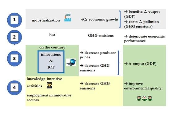
1. Introduction

There have been a lot of studies assessing the impact of new technologies in many sectors, such as schools [1,2], trucking [3], or in emergency medical care ([4], among others). Nevertheless, the effect of information and communication technology (ICT; according to [5], ICT consists of hardware, software, networks and media for storage, collection, processing transmission and presentation of information in the form of data, text, images, and voice. They include phone, radio, television, and the Internet) on aggregate productivity and growth has been scarce.

As ref. [6] argued, productivity is not everything but is almost everything in the long-term. In fact, the national income per person, which is one the main indicators of well-being, is largely conditioned by the labour productivity growth. In recent decades, innovation and ICT have gained prominence as possible drivers of countries’ economic performance ([7,8,9], among others). Authors such as [10,11] or [12] concluded that ICT penetration (ICT penetration refers to the accessibility, security and efficiency of phones, computers, televisions, and radio sets and the several networks that associate them) is the key factor to promote innovation diffusion and therefore economic growth.

In addition, ICT has revolutionized the transfer of technology, knowledge, and information across countries [13]. It is considered as a crucial tool for promoting economic growth and sustainable development, due to the fact that it is a way to improve processes and products. ICT contributes to reducing costs, it helps to overcome distance, and it is a vehicle to achieve more efficiency in firms, industries, and countries ([14,15,16], among others). Some empirical evidence supports the idea that ICT influences economic performance not only at a micro level but also at a macro level (see for instance, [17,18,19]; among others).

Added to that, some decades ago, governments and institutions became concerned with the effects of economic growth on environmental sustainability. In 1955, ref. [20] identified what was a new phenomenon at the time—that is, that the environmental degradation increased with the increments in the Gross Domestic Product (GDP) per capita or income until a particular threshold, and after this point, the environmental degradation started to decrease. More recently, and according to the Fifth Assessment Report of the United Nations Intergovernmental Panel on Climate Change, greenhouse gas (GHG) emissions are considered one of the main causes of global warming since the middle of the last century. One of the most important agenda in the 21st century is to avoid climate change by reducing or replacing energy from fossil fuels, which are the main factor of GHG emissions. This proposal shows evidence on the danger that a non-environmentally friendly economic growth would cause.

The purpose of this paper is twofold. Firstly, we will try to clarify whether ICT favour economic growth. Secondly, we would also like to check whether the contributions of ICT enhance environmental quality, leading to a sustainable economic growth path. Our reasoning is as follows: we will try to test whether the positive impact of ICT on growth is compatible with a (presumable) reduction in GHG emissions. And from that we could infer that the increase in ICT in the production process would be a way to reduce pollution and make the economic growth path more sustainable.

For the empirical application in this study, we will use European Union (EU) data. According to [21], many European countries have undergone relevant economic growth, while others have been characterized by lower productivity and lower economic growth rates. For that reason, the EU would be an interesting case study.

To achieve our aim, the rest of the paper will be as follows. In the next section, we will give a literature review. Next, after relating the data, the used methodology will be explained. After that, we will discuss the empirical results, and finally, we will conclude with a summary and some remarks.

2. Literature Review

2.1. ICT and Economic Growth

Reference [22] claimed that economies which are characterized by easy access to communications network, and institutions that promote knowledge creation and dissemination, would have better economic opportunities. For that reason, developed countries showed more advantages with respect to developing economies. According to [23], there are three channels though which ICT affects economic growth: the adoption of ICT and its productive use in other sectors, the growth effect of the producer of ICT, and finally, innovation and fostering technology diffusion.

Regarding the effects of being a producer of technology, versus adopting technologies from another countries, ref. [24] detected an asymmetric effect. They studied the relationship between the real GDP per capita and the ICT use index for 159 economies throughout the world, and they found that the effects are asymmetric for different groups of countries, depending on whether the countries produce or adopt technologies. In the same line, ref. [25] tried to check whether there were statistically significant differences on the impact of ICT on economic growth, comparing developing, emerging, and developed countries. This author analyzed 59 economies over the period from 1995 to 2010, and he applied panel data regressions and compared their elasticities among these three groups of nations. His results show that emerging and developing countries do not obtain more from investments in ICT than that which is obtained by developed economies. In the same line, taking into account a panel of 123 countries and applying an ICT index from mobile Internet and fixed broadband, ref. [26] identified that ICT contributes to higher economic growth; nevertheless, middle-income and low-income economies tend to attain more from the ICT revolution.

The above empirical results can be supported by the economic theory on international trade. Among the numerous relevant contributions, we could mention [27,28,29,30,31,32,33], among others).

With respect the role of innovations, ref. [34] supported the hypothesis of positive causality between investment in telecommunication infrastructure and economic growth for 21 Organisation for Economic Co-operation and Development (OECD) economies. Applying broadband penetration as a proxy of ICT, ref. [35] found a positive causal nexus between the diffusion on innovation and economic growth. Later, ref. [36] identified that important economic growth occurred during the period 1996–2005 after applying improvements in ICT in a sample of 102 economies, and ref. [37] found that the penetration rates of telecommunication services contribute to a higher efficiency of production. Using a vector error-correction model, ref. [38] studied whether the direction of causality among the diffusion of innovation, penetration of ICT, and economic growth runs both ways, one way, or not at all. Even though, in the short run, the causal link between these variables is not very clear, because it depends on the proxies used, in the long run, innovation diffusion, as well as ICT penetration, significantly contribute to economic growth in European countries. In a more recent study, using the panel vector autoregressive model, ref. [39] showed that both the reinforcement of research and development and the increase in investment in ICT infrastructure contribute to long-term economic performance in the OECD economies during the period 1961–2018.

There are numerous studies analyzing the contributions of ICT to economic growth. A positive contribution of ICT to output was detected by [40], both for richer or less industrialized countries and proportionally to the information and technology (IT) capital.

Reference [41] investigated the impact of high-tech equipment on economic growth for the US and for 15 countries of the EU between 1980 and 2004. He distinguished between three kinds of ICT assets (software, communication equipment, and finally computer and office machinery) and three non-ICT related (transport equipment, non-IT equipment, and non-residential buildings). His results support the growth account perspective, because the leading countries of the EU remain behind the US. He mentioned that a low specialization into innovative production and internal markets characterized by many rigidities can explain the fall in competitiveness.

In the same vein, ref. [42] identified the ICT capital as one of the most relevant explanatory variables explaining the widening productive gap both between EU countries and between the US and Europe. The ICT revolution was crucial to understand the acceleration in output and productivity in the US. According to [43] or [44], this can be explained through three transmission channels. First, the increase in Total Factor Productivity (TFP) in ICT manufacturing industries can be caused by rapid technological progress in the production of ICT goods. Second, the expansion of ICT investment is due to the drop in the ICT goods prices, generating more productive workers. Finally, in general, the ICT spreads with a time lag, becoming pervasive and what is called a general-purpose technology, which can facilitate the introduction of more efficient organizational forms [45].

According to [46], ICT can influence the TFP through several channels. In particular, they identified a direct impact on output, due to the productivity effect which is considered as a precursor for future innovation, and therefore this fact can generate knowledge spillovers. Moreover, authors such as [47,48,49,50,51] supported the idea that investment in ICT reduces communication and production costs, which is crucial to enhancing production procedures and techniques.

Following these lines, and the findings of [44], in this paper, we will study whether technological innovations reduce ICT goods’ producer prices, leading to greater productivity and fostering economic growth.

2.2. Environmental Quality and Economic Growth

According to the Fifth Assessment Report of the United Nations Intergovernmental Panel on Climate Change, greenhouse gas (GHG) emissions are one of the primary causes of global warming that has occurred since the middle of the last century. One of the most important agenda in the 21st century is to avoid climate change by reducing or replacing energy from fossil fuels, which are the main factor of GHG emissions. However, according to [52], the economic and social structure must change to achieve sustainable development.

Reference [20] identified a new phenomenon in which environmental degradation increased with the increment in the GDP per capita or income until a particular threshold, and after this point the environmental degradation started to decrease. The environmental Kuznets curve (EKC) is widely implemented with the purpose of analyzing the nexus between income distribution and environmental population [53,54,55].

Following [56,57], there are three channels to determine whether environmental quality and economic performance show a linear, a U-, or inverted U-shaped nexus. In particular, they distinguished between the scale (volume) of production, composition or means of production, and uses of technology for production. Many studies corroborated that carbon emissions increase given the increasing scale of production (indexed by the GDP growth), keeping the composition of input and technology constant. Based on the composite effects, the EKC justifies that carbon emissions increase taking into account the composition of the production factor with an unchanging volume of technology and economic activities. On the contrary, the use of technology for production maintains that the carbon emissions depend on government regulations and legislation of energy prices.

There have been several authors who have validated the inverted U-shaped link between carbon emissions and economic performance, such as [58,59,60,61,62]. Nevertheless, there is not a consensus. The partial EKC or U-shaped hypothesis was achieved using different estimation techniques, different variables, and different time periods in [63,64].

On the contrary, the inverted U-shaped link was not validated in the USA during the period of 1960–2004 [65], and authors such as [66] did not detect an inverted U-shaped link between the CO₂ emissions per capita and economic growth per capita in Malaysia during the period 1970–2009. Other country-specific studies in which the authors did not find evidence of the EKC phenomenon include [67,68], among others.

The conclusion comparing multiple-country analysis is also not conclusive. In a study of 50 countries considering several development levels, ref. [69] identified different stages of the inverted U-shape curve. A quadratic link was detected by [70] between income and environment for 22 OECD countries applying the pooled mean group estimator. Using a dynamic causality procedure for BRIC countries, ref. [71] detected a short run one-way causality from CO₂ emissions to income between 1971 and 2005. In contrast, ref. [72] did not validate the EKC proposition.

According to [73], the divergence of GHG emissions and economic growth means that after an observed decrease in GHG emissions, the economy grows. It is worth mentioning that there are two different concepts; first, absolute decoupling, which corresponds to when GDP grows but GHG emissions fall, and second, relative decoupling, which it is characterized by higher emissions. Ref. [73] demonstrated that GHG emissions reduction can pose a threat to economic growth. On the other hand, there are several studies, for instance [74,75], in which the authors showed that Western European economies have undergone relevant economic growth, whereas, in contrast, these countries have experienced a decrease trend in their GHG emissions. Using panel data of EU countries and Ukraine for the 2000–2016 period, ref. [76] confirmed the EKC hypothesis.

In contrast to authors such as [77,78], who identified a very firmly coupled relationship between GDP and CO₂ emissions, ref. [79] claimed that the accepted convention in this nexus is ill-founded at the international comparative level. In other words, based on the environmental Kuznets curve, the economic growth and environmental emissions prove to be linked in advanced countries. Nevertheless, in economies with low carbon emissions, this relationship does not work if we compare the data at the international level, applying the fuzzy-set ideal type analysis.

Having those considerations in mind, we are also interested in analyzing the relationship between growth-promoting ICT and the environmental quality. In other words, we would like to study whether the use of ICT promotes growth while preserving the environment.

3. Research Questions and Data

To achieve the aim of this paper, we used EU data. The heterogeneity of the economies of the EU’s member states makes it an interesting region as a case study [21]. We used data on the 27 EU countries over the period of recovery from the financial crisis: from 2008–2018. All the variables were extracted from Eurostat.

In a first step, we checked whether technological innovations reduce producer prices, following the findings of [80] on the relevance of ICT in the USA’s productivity acceleration. Their most significant result is the higher impact on the IT producing sector, and this outcome is due to the fall in IT prices as the main factor.

In the second step, our dependent variable was the real growth rate of GDP. In this instance, our aim was to study the impact of innovations on economic growth.

The independent variables related to ICT, which presumably foster economic growth, were those that represent innovation and the evolution of IT prices. To consider proxies for the innovation indicator variables, we followed [81]. In particular, technological progress has been captured by high-technology products exports as a share of total exports; the high-technology sector’s employment as a percentage of total employment; knowledge-intensive high-technology services’ employment as a percentage of total employment, and employment in information and communication technology as a percentage of total employment. To capture the average change over time in the selling prices received by domestic producers for their output, we considered the producer price index in industry. Moreover, we considered different price level indices such as communication; audio-visual, photographic, and information processing equipment; machinery and equipment; software; electrical and optical equipment; durable goods; and capital goods prices. Additionally, we considered some macroeconomic variables as control variables, such as population growth rate, gross fixed capital formation, inflation rate, and degree of openness. These variables were taken from the World Development Indicators.

Finally, we tried to analyze the relationship among the variables that foster economic growth and environmental quality. In other words, we aimed to answer the question of whether the penetration and use of ICT contribute not only to promoting economic growth, but also to improving the environment. Given the relevance of GHG on global warming, as stated in the literature section, we will include the GHG emissions as an alternative variable of our data set. There are several studies in which the GHG have proven to play a crucial role in the economic growth performance, as can be seen, for instance, in [82,83,84,85] and [58], among others.

4. Methodology

Given the nature of our data set, we applied panel data techniques to perform our estimations following [86,87,88].

To answer our first research question, the first equation defines the producer prices as a function of innovation indicators.

$$P{P}_{it}=\alpha +{\beta }_{1}Exp\_hightec{h}_{it}+{\beta }_{2}Empl\_x{x}_{it}+{\epsilon }_{it}$$

(1)

where $P{P}_{it}$ is the producer prices and $Exp\_hightec{h}_{it}$ represents the exports of high-technology products as a share of total exports. Aiming to check the robustness of our results, we used three alternative measures of employment ($Empl\_x{x}_{it}$) such as the high-technology sector’s employment rate, the knowledge-intensive high-technology services, and the information and communication technology employment rate. These three variables are measured as a percentage of total employment.

Next, to study the contribution of ICT to growth, we will estimate the following extended economic growth equation based on the neoclassical growth model:

$$g_{it}=\alpha +{\displaystyle \sum }_{j=1}^n{\delta }_{ij}{X}_{ijt}+{\beta }_{1}P{P}_{it}+{\beta }_{2}PL{I}_{it}+{\beta }_{3}innov\_indicator{s}_{it}+{\epsilon }_{it}$$

(2)

where $g_{it}$ is the per capita GDP, $P{P}_{it}$ is the producer prices, $PLI price{s}_{it}$ is the price level index, $innov\_indicator{s}_{it}$ represents the innovation indicators, and ${\epsilon }_{it}$ denotes the error term. Regarding X_it, we consider a set of explanatory variables that have been shown to be consistently associated with growth in the literature (see [89] for a comprehensive account of the most important contributions and debates on growth): population growth rate as a percentage (POPGR_it); the ratio of gross fixed capital formation to GDP (GKF_it); openness to trade, measured by the sum of exports and imports over GDP (OPEN_it); and the GDP deflator inflation rate, a measure of macroeconomic instability and uncertainty (INF_it). The initial level of initial real per capita GDP is also introduced in Equation (1) to capture the conditional convergence of the economy to its steady state.

Finally, to check whether the contributions of ICT to economic growth favor environmental quality, we analyze the relationship between some innovation indicators and the GHG emissions, as shown in Equation (3).

$$GH{G}_{it}=\alpha +{\beta }_{1}Exp\_hightec{h}_{it}+{\beta }_{2}Empl\_x{x}_{it}+{\epsilon }_{it}$$

(3)

where $GH{G}_{it}$ represents the greenhouse gas emissions and $Exp\_hightec{h}_{it}$ is the exports of high-technology products as a share of total exports. $Empl\_x{x}_{it}$ focuses on the high-technology sector’s employment, the knowledge-intensive high-technology services, and the information and communication technology employment as a percentage of total employment. As in Equation (1), we use three different measures of employment in the innovation sector to check the robustness of our results.

When the explanatory variables in the regression model are not stationary, the standard assumptions for asymptotic analysis are not reliable. That means that we cannot apply the hypothesis tests, and consequently the panel unit root tests should be applied. Specifically, we use the [90,91,92,93,94] tests. According to

Table 1. Panel unit root tests.

	Level
Test Statistics	Economic Growth	Exports High Technology	Employment in High-Technology	Employment in Knowledge-Intensive High-Technology	Employment in Information and Communication	PP	Greenhouse Gas Emissions	POPGROW	GKF	INF	OPEN
LLC
Level	−15.1429 (0.0000)	−9.0390 (0.0000)	−7.1451 (0.0000)	−7.2279 (0.0000)	−8.9595 (0.0000)	−12.2807 (0.0000)	−5.5727 (0.0000)	−3.9300 (0.0000)	−9.3934 (0.0000)	−8.9166 (0.0000)	−17.3962 (0.0000)
Trend	−20.2548 (0.0000)	−6.2019 (0.0000)	−9.6222 (0.0000)	−11.3476 (0.0000)	−12.4290 (0.0000)	−15.5713 (0.0000)	−10.3223 (0.0000)	−10.0201 (0.0000)	−14.8569 (0.0000)	−9.8176 (0.0000)	−11.1120 (0.0000)
HT
Level	0.2904 (0.0000)	0.7887 (0.7858)	0.4939 (0.0000)	0.4426 (0.0000)	0.4200 (0.0000)	−0.0987 (0.0000)	0.6609 (0.0340)	0.6519 (0.0223)	0.5178 (0.0000)	0.2429 (0.0000)	0.7620 (0.5971)
Trend	0.1717 (0.0000)	0.2132 (0.0006)	0.2315 (0.0014)	0.1708 (0.0000)	0.2016 (0.0003)	−0.1670 (0.0000)	0.4094 (0.4157)	0.3533 (0.1389)	0.3022 (0.0301)	0.1472 (0.0000)	0.3998 (0.3588)
Breitung
Level	−7.1897 (0.0000)	1.2878 (0.9011)	2.9267 (0.9983)	1.8119 (0.9650)	2.6465 (0.9959)	−5.2659 (0.0000)	0.9962 (0.8404)	0.3131 (0.6229)	−1.0782 (0.1405)	−2.4057 (0.0081)	−0.8109 (0.2087)
Trend	−6.6495 (0.0000)	−0.2685 (0.3942)	−2.1177 (0.0171)	−3.6308 (0.0001)	−4.1080 (0.0000)	−2.2642 (0.0118)	−0.0293 (0.4883)	3.0070 (0.9987)	1.4798 (0.9305)	−0.7003 (0.2419)	−2.9325 (0.0017)
IPS
Level	−4.0086 (0.0000)	−0.4050 (0.3427)	−2.0079 (0.0223)	−2.2953 (0.0109)	−2.5063 (0.0061)	−6.5728 (0.0000)	−1.7695 (0.0384)	−0.3508 (0.3629)	−4.0077 (0.0000)	−6.0474 (0.0000)	−0.2813 (0.3892)
Trend	−5.7496 (0.0000)	−2.4858 (0.0065)	−3.1423 (0.0008)	−3.6573 (0.0001)	−3.5728 (0.0002)	−6.4491 (0.0000)	−3.8719 (0.0001)	−1.0454 (0.1479)	−2.7043 (0.0034)	−4.4589 (0.0000)	−0.7599 (0.2237)
Fisher
Level	4.6334 (0.0000)	0.7975 (0.2126)	12.7333 (0.0000)	15.6291 (0.0000)	6.2934 (0.0000)	4.2036 (0.0000)	−0.9832 (0.8372)	1.4351 (0.0756)	8.1558 (0.0000)	6.1770 (0.0000)	4.9927 (0.0000)
Trend	5.7487 (0.0000)	−1.9772 (0.9760)	15.4283 (0.0000)	30.7267 (0.0000)	14.8060 (0.0000)	0.1391 (0.4447)	−3.0959 (0.9990)	2.2059 (0.0137)	4.1056 (0.0000)	1.2351 (0.1084)	4.0112 (0.0000)
	Level
Test Statistic	Communication Prices	Audio Prices	Machinery Prices	Electrical Prices	Software Prices	Durable Goods Prices	Capital Goods Prices
LLC
Level	−7.6510 (0.0000)	−4.9112 (0.0000)	−8.9885 (0.0000)	−8.1707 (0.0000)	−13.2777 (0.0000)	−5.7774 (0.0000)	−4.4491 (0.0000)
Trend	−10.3705 (0.0000)	−8.5856 (0.0000)	−15.4493 (0.0000)	−12.8485 (0.0000)	−16.2574 (0.0000)	−9.2569 (0.0000)	−26.7447 (0.0000)
HT
Level	0.7550 (0.5404)	0.0559 (0.0000)	0.5461 (0.0000)	0.5473 (0.0000)	0.4833 (0.0000)	0.5092 (0.0000)	0.6547 (0.0255)
Trend	0.3290 (0.0718)	−0.1012 (0.0000)	0.4862 (0.8369)	0.3577 (0.1546)	0.2563 (0.0048)	0.3753 (0.2288)	0.4066 (0.3986)
Breitung
Level	1.6545 (0.9510)	−4.3833 (0.0000)	−0.6653 (0.2529)	−1.5317 (0.0628)	−1.0480 (0.1473)	−1.1327 (0.1287)	−1.0627 (0.1440)
Trend	−2.5060 (0.0061)	−3.6541 (0.0001)	−0.4640 (0.3213)	−0.9592 (0.1687)	−0.7134 (0.2378)	−1.3460 (0.0891)	−0.1944 (0.4229)
IPS
Level	0.4692 (0.6805)	−5.3416 (0.0000)	−1.3533 (0.0880)	−2.3055 (0.0106)	−1.9055 (0.0284)	−3.3831 (0.0004)	−1.2972 (0.0973)
Trend	−3.4419 (0.0003)	−6.0374 (0.0000)	−1.7958 (0.0363)	−3.5121 (0.0002)	−2.7901 (0.0026)	−4.2392 (0.0000)	−3.7152 (0.0001)
Fisher
Level	1.8167 (0.0346)	−2.3352 (0.9902)	1.9661 (0.0246)	0.3963 (0.3459)	0.0804 (0.4680)	0.4492 (0.3267)	1.5737 (0.0578)
Trend	4.0839 (0.0000)	−2.5861 (0.9951)	−0.9895 (0.8388)	3.0246 (0.0012)	8.4653 (0.0000)	−1.6632 (0.9519)	2.4129 (0.0079)

Note: Numbers in parenthesis are p-values.

, the results of these tests decisively reject the null hypothesis of a unit root for $emp\_hightec{h}_{it}$,$P{P}_{it}, GK{F}_{it}$, $IN{F}_{it}$,$Elec\_price{s}_{it}$, and $Green\_emis{s}_{it}$ (indicating that they are stationary in levels, i.e., I(0)), while they do not reject the null for $exp\_hightec{h}_{it}$ and $OPE{N}_{it}$ (suggesting that these variables can be treated as first-difference stationary, i.e., I(1)).

In particular, we considered three basic panel regression methods: the fixed-effects (FE) method, the random effects (RE) model, and the pooled ordinary least square (POLS) method. To determine the empirical relevance of each of the potential methods for our panel data, we made use of several statistic tests. Specifically, we tested FE versus RE using the Hausman test statistic to test for non-correlation between the unobserved effect and the regressors. To choose between POLS and RE, we used Breusch and Pagan [95]’s Lagrange multiplier test to test for the presence of an unobserved effect. Finally, we used the F test for fixed effects to test whether all unobservable individual effects are zero, to discriminate between POLS and FE. Additionally, we treated the potential endogeneity in our estimations by applying the fixed effects two-step least squares (FE-2SLS) test, the so-called fixed effects instrumental variables (FE-IV) test and the random effects two-step least squares (RE-2SLS) test, or the so-called random effects instrumental variables (RE-IV) test.

5. Empirical Results

Table 2. Producer prices as a function of innovation indicators: All European countries.

KERRYPNX	Model 1	Model 2	Model 3
$Exp\_hightec{h}_{it}$	−0.1517 * (0.0852)	−0.1473 * (0.0853)	−0.1506 * (0.0849)
$Empl\_hightec{h}_{it}$	−0.0991 ** (0.0446)
$Empl\_knowledg{e}_{it}$		−0.0793 ** (0.0412)
$Empl\_IC{T}_{it}$			−0.0939 *** (0.0391)
Constant	7.3072 *** (2.2546)	6.9528 *** (2.3631)	7.5907 *** (2.2247)
Country FE	Yes	Yes	Yes
Year FE	Yes	Yes	Yes
N	297	297	297
R2 overall	0.0106	0.0116	0.0141
R2 within	0.0258	0.0215	0.0288
R2 between	0.0106	0.0507	0.0399
BIC	1707.79	1709.12	1706.89
AIC	1696.71	1698.03	1695.81

Source: Authors’ own elaboration. Notes: In the ordinary brackets below the parameter estimates are the corresponding z-statistics, computed using [96] heteroskedasticity-robust standard errors. *, **, and *** indicate significance at 10%, 5%, and 1%, respectively. In this table, we provide the best method of estimation (which in our case is the fixed effects) after it was applied in the corresponding tests.

offers the results of the estimated producer prices calculated by Equation (1) as a function of innovation indicators. This table offers the FE estimations because, according to the Breusch and Pagan test, the F test for fixed effects and the Hausman test, it is the best method of estimation (the results of RE and POLS estimations and tests are available from the authors upon request). However, as a robustness exercise, three different measures of employment in innovative sectors were used as displayed by the three estimated models.

Clearly, the higher the high-technology exports are, the lower producer prices are. That is to say, technological progress contributes to decreasing producer prices. Moreover, regardless of the instrument used to measure the employment in high-technology sectors, there is a negative relationship between them. In other words, the producer prices will decrease with greater knowledge-intensive activities or employment in innovative sectors.

Once we showed that technological progress has contributed to lower prices of production, our next step was to analyze how producer prices and different price level indices can influence economic growth.

Table 3. Parameter estimates for the empirical model: All European countries in the sample.

Explanatory Factors	FE	RE	POLS	FE-2SLS	RE-2SLS
$g_{it-1}$	0.2015 *** (0.0608)	0.4146 *** (0.0525)	0.4146 *** (0.0525)	0.1360 ** (0.0620)	0.3170 *** (0.0554)
$\Delta \exp \_hightec{h}_{it}$	0.1552 * (0.0938)	0.0581 (0.0923)	0.0581 (0.0923)	0.4147 * (0.2376)	0.6905 (0.6683)
$\mathrm{emp}\_hightec{h}_{it}$	3.6204 *** (0.6258)	0.3920 *** (0.1484)	0.3920 *** (0.1484)	2.6285 *** (1.0045)	0.2959 * (0.1655)
$P{P}_{it}$	0.2496 *** (0.0631)	0.2479 *** (0.0640)	0.2479 *** (0.0640)	0.1384 ** (0.0712)	0.0994 (0.0802)
$GK{F}_{it}$	0.2278 *** (0.0897)	0.1023 * (0.0588)	0.1023 * (0.0588)	0.2179 *** (0.0911)	0.2505 *** (0.0908)
$IN{F}_{it}$	−0.7897 *** (0.1520)	−0.7835 *** (0.1489)	−0.7835 *** (0.1489)	−0.7116 *** (0.1712)	−0.7110 *** (0.1905)
$\Delta OPE{N}_{it}$	0.1307 *** (0.0236)	0.1555 *** (0.0238)	0.1555 *** (0.0238)	0.0514 ** (0.0268)	0.0579 ** (0.0293)
$Elec\_price{s}_{it}$	0.1556 *** (0.0475)	0.0715 ** (0.0327)	0.0715 ** (0.0327)	0.1174 *** (0.0501)	0.0143 (0.0332)
Constant	−17.6796 *** (3.4449)	−2.2100 ** (1.2017)	−2.2100 * (1.017)		−5.6058 (3.7971)
Country FE	Yes	Yes	Yes	Yes	Yes
Year FE	Yes	Yes	Yes	Yes	Yes
N	270	270	270	243	243
R2 overall	0.2202	0.4300	0.4300	0.2709	0.2323
R2 within	0.4608	0.3901		0.1856	0.1308
R2 between	0.3402	0.6490		0.5204	0.5488
BIC	1322.72	1320.60	1382.92	1125.73	1235.68
AIC	1293.93	1300.85	1354.13	1097.79	1147.99
Breusch and Pagan test (POLS vs. RE)	0.00 [1.0000]			Endogeneity test of regressors	8.184 [0.0167]
F test for fixed effects (POLS vs. FE)	2.27 [0.0007]			Weak identification test (Cragg-Donald Wald F statistic)	16.705 10%: 7.03 15%: 4.58 20%: 3.95 25%: 3.63
Haussman test (FE vs. RE)	97.38 [0.0000]			Haussman test (FE-2SLS vs. RE-2SLS)	56.34 [0.0000]
				Underidentification test	29.894 [0.0000]
				Overidentification test (Sargan statistic)	[0.0000]

Source: Authors’ own elaboration. In the ordinary brackets below the parameter estimates are the corresponding z-statistics, computed using [96] heteroskedasticity-robust standard errors. In the square brackets below the specification tests are the associated p-values. *, ** and *** indicate significance at 10%, 5%, and 1%, respectively.

offers the estimation results of Equation (2) controlling for the usual economic factors considered in the economic growth literature such as gross fixed capital formation, inflation rate, or openness. The initial level of initial real per capita GDP is also introduced in Equation (2) to capture the conditional convergence of the economy to its steady state. This table shows the estimation results using the pooled OLS, RE, and FE methodologies. According to the Breusch and Pagan test, F-test for fixed effects, and the Hausman test, the best method of estimation is the FE method. Nevertheless, according to the endogeneity test’s result, we can clearly reject the null hypothesis, meaning that the regressors cannot be treated as exogeneous. To overcome the endogeneity problem, the FE-2SLS and the RE-2SLS estimations are crucial. Based on the Hausman test between FE-2SLS and RE-2SLS, the former is the most appropriate.

As expected, and regardless of the applied method, the lagged economic growth positively influences the actual real growth rate. With respect to the innovation indicators, as can be seen, the high-technology exports promote economic growth. One of the factors which largely contribute to economic growth is the employment in high-technology sectors, at 1% significance level, and it is the most important factor in terms of marginal effects. It is very common that in the long run, more outward-oriented economies are associated with better economic growth (see, for instance, [97,98,99,100,101], among others), and our results support this statement. In the same line, gross fixed capital formation is positively linked to economic growth (as stressed by [102,103,104], among others). On the contrary, inflation rate deteriorates economic growth (the same conclusion was achieved by [105,106], among others). We also found that producer prices and price level indices such as electrical prices (as a measure of robustness, we introduced different price level indices, such as communication; audio-visual, photographic and information processing equipment; machinery and equipment; software; durable goods; and capital goods prices. However, only the electrical and optical equipment prices indices are statistically significant) reveal a negative nexus with real economic growth.

In addition, we offer the underidentification test, which is an LM test of analyzing if the equation is identified—this means that the excluded instruments are relevant. In particular, we have enough evidence to reject the null hypothesis in which the equation is underidentified, meaning that the model is identified. The weak identification test is very similar to the previous one; however, in this case, we test whether the excluded instruments are correlated with the endogeneous regressors, but only weakly. In the table, we show the compiled critical values for the Cragg–Donald F statistic for instrumental variables by [107]. As this F statistic is greater than the critical values, this implies that our instruments have the explanatory power for explaining the endogeneous variables. Finally, using the Sargan–Hansen test, which is a test of overidentifying restrictions, we reject the null hypothesis.

To complete our analysis, as previously mentioned, a topic of major concern worldwide is the growing trend of greenhouse gas emissions. Due to the relevant implications that they have on climate change, EU27 leaders agreed to reduce GHG emissions by at least 55% by 2030. Having those considerations in mind,

Table 4. Parameter estimates for the empirical model: all European countries in the sample (with greenhouse gas emissions).

Explanatory Factors	FE	RE	POLS	FE-2SLS	RE-2SLS
$g_{it-1}$	0.1744 *** (0.0627)	0.4098 *** (0.0532)	0.4098 *** (0.0532)	0.1252 ** (0.0655)	0.3161 *** (0.0555)
$\Delta \exp \_hightec{h}_{it}$	0.1500 (0.0938)	0.0563 (0.0925)	0.0563 (0.0925)	0.4250 * (0.2390)	0.6896 (0.6676)
$\mathrm{emp}\_hightec{h}_{it}$	3.7678 *** (0.6296)	0.4073 *** (0.1509)	0.4073 *** (0.1509)	2.7012 *** (1.0334)	0.2992 * (0.1661)
$P{P}_{it}$	0.2448 *** (0.0629)	0.2484 *** (0.0641)	0.2484 *** (0.0641)	0.1477 ** (0.0721)	0.1002 (0.0799)
$GK{F}_{it}$	0.2668 *** (0.0923)	0.1137 * (0.0620)	0.1137 * (0.0620)	0.2330 *** (0.0950)	0.2529 *** (0.0968)
$IN{F}_{it}$	−0.6934 *** (0.1620)	−0.7711 *** (0.1506)	−0.7711 *** (0.1506)	−0.6862 *** (0.1781)	−0.7091 *** (0.1898)
$\Delta OPE{N}_{it}$	0.1273 *** (0.0236)	0.1548 *** (0.0238)	0.1548 *** (0.0238)	0.0503 * (0.0269)	0.0579 ** (0.0294)
$Elec\_price{s}_{it}$	0.1513 *** (0.0475)	0.0711 ** (0.0327)	0.0711 ** (0.0327)	0.1171 ** (0.0502)	0.0143 (0.0333)
$Green\_emis{s}_{it}$	−0.0705 * (0.0422)	−0.0145 (0.0247)	−0.0145 (0.0247)	−0.0333 * (0.0478)	−0.0029 (0.0252)
Constant	−12.6312 *** (4.5685)	−1.1793 (2.1326)	−1.1793 (2.1326)		−5.3944 (4.1382)
Country FE	Yes	Yes	Yes	Yes	Yes
Year FE	Yes	Yes	Yes	Yes	Yes
N	270	270	270	243	243
R2 overall	0.2164	0.4307	0.4307	0.1656	0.2325
R2 within	0.4672	0.3921			0.1311
R2 between	0.3250	0.6432			0.5493
BIC	1325.13	1322.18	1388.16	1132.76	1256.81
AIC	1292.74	1296.80	1355.77	1101.32	1186.52
Breusch and Pagan test (POLS vs. RE)	0.00 [1.0000]			Endogeneity test of regressors	8.235 [0.0163]
F test for fixed effects (POLS vs. FE)	2.38 [0.0004]			Weak identification test (Cragg-Donald Wald F statistic)	16.483 10%: 7.03 15%: 4.58 20%: 3.95 25%: 3.63
Haussman test (FE vs. RE)	290.54 [0.0000]			Haussman test (FE-2SLS vs. RE-2SLS)	56.07 [0.0000]
				Underidentification test	29.673 [0.0000]
				Overidentification test (Sargan statistic)	[0.0000]

Source: Authors’ own elaboration. In the ordinary brackets below the parameter estimates are the corresponding z-statistics, computed using [96] heteroskedasticity-robust standard errors. In the square brackets below the specification tests are the associated p-values. *, ** and *** indicate significance at 10%, 5%, and 1%, respectively.

again offers the estimation of Equation (2), but now incorporating the GHG emissions to analyze their impact on real economic growth. According to the Hausman test, the best estimation method is the FE-2SLS (FE-IV) method after controlling for endogeneity, which reveals that there exists a negative and statistically significant effect of GHG emissions on economic performance. The employment in high-technology sectors still remains the most important explanatory variable for the real economic growth rate, followed by the exports of high-technology products. As expected, the gross capital formation rate highly contributes to higher economic activity. A positive relationship between producer prices, degree of openness, and electrical prices is detected with the economic growth. On the contrary, a statistically significant negative link is identified between inflation rate and economic performance.

Finally, to check whether the contributions of ICT to economic growth favour environmental quality, we will estimate the GHG emissions as a function of innovation indicators According to Equation (3).

Table 5. Greenhouse gas (GHG) emissions as a function of innovation indicators: All European countries.

Explanatory Factors	Model 1	Model 2	Model 3
$Exp\_hightec{h}_{it}$	0.4368 *** (0.1091)	0.4518 *** (0.1112)	0.4475 *** (0.1070)
$Empl\_hightec{h}_{it}$	−0.5530 *** (0.0572)
$Empl\_knowledg{e}_{it}$		−0.4771 *** (0.0537)
$Empl\_IC{T}_{it}$			−0.5077 *** (0.0493)
Constant	103.5522 *** (2.8863)	103.3523 *** (3.0812)	104.3183 *** (2.8046)
Country FE	Yes	Yes	Yes
Year FE	Yes	Yes	Yes
N	297	297	297
R2 overall	0.0537	0.1372	0.1309
R2 within	0.3151	0.2864	0.3378
R2 between	0.0373	0.1404	0.1285
BIC	1854.51	1866.72	1844.50
AIC	1843.43	1855.63	1833.42

Source: Authors’ own elaboration. In the ordinary brackets below the parameter estimates are the corresponding z-statistics, computed using [96] heteroskedasticity-robust standard errors. *, **, and *** indicate significance at 10%, 5%, and 1%, respectively. In this table, we provide the best method of estimation (that in our case is the fixed effects) after it have been applied the corresponding tests.

shows the estimation results. This table offers only the FE estimations because, according to the Breusch and Pagan test, the F test for fixed effects and the Hausman test, this is the best method of estimation (the results of RE and POLS estimations and tests are available from the authors upon request). However, as a robustness exercise, three different measures of employment in innovative sectors has been used, as displayed by the three estimated models.

On one hand, as can be seen, there exists a positive relationship between exports of high-technologies and the GHG emissions. On the other hand, and regardless of the model used, a consensus conclusion could be achieved: the higher the employment in high-technology sectors, and the greater the employment related to knowledge-intensive activities or employment in ICT sectors, the lower the environmental degradation. In other words, when the employment related to innovations increases, the GHG decreases, which presumably improves the environmental quality.

6. Conclusions

For the last few decades, governments and institutions have been concerned with the effects of economic growth on environmental sustainability. Pollution is one of the costs of economic growth, and GHG emissions are a product derived from industrialization and the massive production of goods. The growing concern relating to the danger that economic growth could pose to the environment has occurred in parallel with the development of new technologies. ICT enhances economic growth, but one might wonder whether ICT could represent a way of reducing pollution to sustainable levels.

Taking that into account, in this paper, we have tested whether the positive impact of ICT on growth is compatible with a reduction in GHG emissions. First, and following [80]’s proposal, we have analyzed the ways in which ICT contributes to growth—that is, reducing producer prices and favoring productivity. Applying panel data techniques on the 27 EU during the period from 2008 to 2018, the first step of our study tries to explain the relationship between innovation indicators and producer prices. In particular, the higher the exports of high-technology products, the lower the producer prices. In addition, considering three alternative measures of employment related to this sector (high-technology sector, high-technology services, or ICT employment), the conclusion is a very consensual. This that the more resources the economy allocates to investing in more ICT employment, the lower the producer prices. Controlling for the usual explanatory variables such as gross capital formation, openness degree, and inflation rate, we extended the neoclassical growth model trying to analyze the effect of ICT on economic performance. The estimation results are very clear. ICT leads to higher per capita economic growth. In the second step of the analysis, we analyze the relationship between some innovation indicators and the GHG emissions. We found that GHG emissions can erode the economic growth, and, more precisely, that the exports of high-technology products can generate more GHG emissions in the European countries. However, greater ICT employment can significantly reduce the GHG emissions, leading to a better environmental quality.

With due caution, our results could suggest that ICT not only reduces costs and improves efficiency, fostering economic growth, but also the increase in activities related to ICT performance contributes to reducing GHG emissions. That is the case of employment in high-technology sectors, the employment related to knowledge-intensive activities or even direct employment in the ICT sector. Currently, the use of new technologies is revolutionizing the labor market, which represents an opportunity to reconvert the industrial and services sector towards more efficient production which is also less harmful to the environment.

A direct implication for economic policies would be the promotion of the research and the adoption of technology, mainly in readjusting jobs towards the ICT sector and encouraging and supporting the training of workers in technological skills.

References

- Angrist, J.; Lavy, V. New evidence on classroom computers and pupil learning. Econ. J. 2002, 112, 735–765. [Google Scholar] [CrossRef] [Green Version]
- Machin, S.; McNally, S.; Silva, O. New Technology in Schools: Is There a Payoff? Econ. J. 2007, 117, 1145–1167. [Google Scholar] [CrossRef]
- Baker, G.; Hubbard, T. Contractability and asset ownership: On board computers and governance in US trucking. Q. J. Econ. 2004, 119, 1443–1480. [Google Scholar] [CrossRef]
- Athey, S.; Stern, S. The impact of information technology on emergency health care outcomes. Rand J. Econ. 2002, 33, 399–432. [Google Scholar] [CrossRef]
- World Bank. ICT and MDGs: A World Bank Group Perspective; The World Bank: Washington, DC, USA, 2003. [Google Scholar]
- Krugman, P. The Age of Diminished Expectations, 3rd ed.; U.S. Economic Policy in the 1990s; MIT Press: Cambridge, MA, USA, 1997; p. 11, Chapter 1. [Google Scholar]
- Avgerou, C. Information systems in developing countries: A critical research review. J. Inf. Technol. 2008, 23, 133–146. [Google Scholar] [CrossRef] [Green Version]
- Jha, A.K.; Bose, I. Innovation research in information systems: A commentary on contemporary trends and issues. Inf. Manag. 2016, 53, 297–306. [Google Scholar] [CrossRef]
- Hudson, J.; Minea, A. Innovation, intellectual property rights and economic development: A unified empirical investigation. World Dev. 2013, 46, 66–78. [Google Scholar] [CrossRef]
- Dedrick, J.; Gurbaxani, V.; Kraemer, K.L. Information technology and economic performance: A critical review of the empirical evidence. ACM Comput. Surv. 2003, 35, 1–28. [Google Scholar] [CrossRef]
- Dutta, S.; Shalhoub, Z.K.; Samuels, G. Promoting Technology and Innovation: Recommendations to Improve Arab ICT Competitiveness; The Arab World Competitiveness Report, 81–96; World Economic Forum: Geneva, Switzerland, 2007. [Google Scholar]
- Cardona, M.; Kretschmer, T.; Strobel, T. ICT and productivity: Conclusions from the empirical literature. Inf. Econ. Policy 2013, 25, 109–125. [Google Scholar] [CrossRef]
- Chen, D.H.C.; Kee, H.L. A Model on Knowledge and Endogenous Growth; World Bank Policy Research Working Paper, No. 3539; The World Bank: Washington, DC, USA, 2005. [Google Scholar]
- Cuervo, M.R.V.; Menendez, A.J.L. A multivariate framework for the analysis of the digital divide: Evidence from the European Union-15. Inf. Manag. 2006, 43, 756–766. [Google Scholar] [CrossRef]
- OECD. OECD Information Technology Outlook 2010; Organisation for Economic Co-Operation and Development: Paris, France, 2010. [Google Scholar]
- Arvanitis, S.; Loukis, E.; Diamantopoulou, V. The effect of soft ICT capital on innovation performance of Greek firms. J. Enterp. Inf. Manag. 2013, 26, 679–701. [Google Scholar] [CrossRef]
- Zhang, F.; Li, D. Regional ICT access and entrepreneurship: Evidence from China. Inf. Manag. 2018, 55, 188–198. [Google Scholar] [CrossRef]
- Vu, K.M. Information and communication technology (ICT) and Singapore’s economic growth. Inf. Econ. Policy 2013, 25, 284–300. [Google Scholar] [CrossRef]
- Sassi, S.; Goaied, M. Financial development, ICT diffusion and economic growth: Lessons from MENA region. Telecommun. Policy 2013, 37, 252–261. [Google Scholar] [CrossRef]
- Kuznets, S. Economic growth and income inequality. Am. Econ. Rev. 1955, 45, 1–28. [Google Scholar]
- Veugelers, R. An innovation deficit behind Europe’s overall productivity slowdown? In Proceedings of the Investment and Growth in Advanced Economies Conference Proceedings, European Central Bank Forum on Central Banking, Sintra, Portugal, 26–28 June 2017. [Google Scholar]
- Braga, C.; Fink, C.; Sepulveda, C. Intellectual Property Rights and Economic Development; World Bank TechNet Working Paper; World Bank: Washington, DC, USA, 1998. [Google Scholar]
- Van Ark, B. Measuring the new economy: An international comparative perspective. Rev. Income Wealth 2002, 48, 1–14. [Google Scholar] [CrossRef]
- Farhadi, M.; Fooladi, M. The impact of information and communication technology use on economic growth. In International conference on Humanities, Society and Culture IPEDR; IACSIT Press: Singapore, 2011; Volume 20. [Google Scholar]
- Niebel, T. ICT and economic growth-comparing developing, emerging and developed countries. World Dev. 2018, 104, 197–211. [Google Scholar] [CrossRef] [Green Version]
- Appiah-Otoo, I.; Song, N. The impact of ICT on economic growth-comparing rich and poor countries. Telecommun. Policy 2021, 45, 102082. [Google Scholar] [CrossRef]
- Findlay, R. Relative Backwardness, Direct Foreign Investment, and the Transfer of Technology: A Simple Dynamic Model. Q. J. Econ. 1978, 92, 1–16. [Google Scholar] [CrossRef]
- Findlay, R. Some Aspects of Technology and Direct Foreign Investment. Am. Econ. Rev. Pap. Proc. 1978, 68, 275–279. [Google Scholar]
- Johnson, H.G. Technological Change and Comparative Advantage: An Advanced Country’s Viewpoint. J. World Trade Law 1975, 9, 1–14. [Google Scholar]
- Jones, R.W.; Neary, J.P. The Role of Technology in the Theory of International Trade. In The Technology Factor in International Trade; Vernon, R., Ed.; NBER: New York, NY, USA, 1970; pp. 95–127. [Google Scholar]
- Jones, R.W.; Neary, J.P. The Positive Theory of International Trade. In Handbook of International Economics; Elsevier: Amsterdam, The Netherlands, 1984; pp. 1–62. [Google Scholar]
- Krugman, P. A Model of Innovation, Technology Transfer, and the World Distribution of Income. J. Political Econ. 1979, 87, 253–266. [Google Scholar] [CrossRef]
- Markusen, J.R.; Svensson, L. Trade in Goods and Factors with International Differences in Technology; Working Paper No. 1101; National Bureau of Economic Research: Cambridge, MA, USA, 1983. [Google Scholar]
- Röller, L.H.; Waverman, L. Telecommunications infrastructure and economic development: A simultaneous approach. Am. Econ. Rev. 2001, 91, 909–923. [Google Scholar] [CrossRef] [Green Version]
- Koutroumpis, P. The economic impact of broadband on growth: A simultaneous approach. Telecommun. Policy 2009, 33, 471–485. [Google Scholar] [CrossRef]
- Vu, K.M. ICT as a source of economic growth in the information age: Empirical evidence from the 1996–2005 period. Telecommun. Policy 2011, 35, 357–372. [Google Scholar] [CrossRef]
- Thompson, H.G.; Garbacz, C. Economic impacts of mobile versus fixed broadband. Telecommun. Policy 2011, 35, 999–1009. [Google Scholar] [CrossRef]
- Pradhan, R.P.; Arvin, M.B.; Nair, M.; Bennett, S.E.; Hall, J.H. The information revolution, innovation diffusion and economic growth: An examination of causal links in European countries. Qual. Quant. 2019, 53, 1529–1563. [Google Scholar] [CrossRef]
- Nair, M.; Pradhan, R.P.; Arvin, M.B. Endogenous dynamics between R&D, ICT and economic growth: Empirical evidence from the OECD countries. Technol. Soc. 2020, 62, 101315. [Google Scholar]
- Park, J.; Shin, S. The Maturity and Externality Effects of Information Technology Investments on National Productivity Growth; Working Paper Series 2004-05 No. 2; University of Rhode Island, College of Business Administration: South Kingstown, Rhode Island, 2004. [Google Scholar]
- Venturini, F. ICT and productivity resurgence: A growth model for the information age. BE J. Macroecon. 2007, 7, 1–26. [Google Scholar] [CrossRef] [Green Version]
- Seo, H.J.; Lee, Y.S.; Oh, J.H. Does ICT investment widen the growth gap? Telecommun. Policy 2009, 33, 422–431. [Google Scholar] [CrossRef]
- Jorgenson, D.W.; Stiroh, K.J. US economic growth at the industry level. Am. Econ. Rev. 2000, 90, 161–168. [Google Scholar] [CrossRef] [Green Version]
- Oliner, S.D.; Sichel, D.E. The resurgence of growth in the late 1990s: Is information technology the story? J. Econ. Perspect. 2000, 14, 3–22. [Google Scholar] [CrossRef] [Green Version]
- David, P. They dynamo and the computer: An historical perspective on the modern productivity paradox. Am. Econ. Rev. 1990, 80, 355–361. [Google Scholar]
- Becchetti, L.; Adriani, F. Does the digital divide matter? The role of information and communication technology in cross-country level and growth estimates. Econ. Innov. New Technol. 2005, 14, 435–453. [Google Scholar] [CrossRef] [Green Version]
- Stiroh, K.J. Are spillovers driving the new economy? Rev. Income Wealth 2002, 48, 33–57. [Google Scholar] [CrossRef]
- Galperin, H. Wireless networks and rural development: Opportunities for Latin America. Inf. Technol. Int. Dev. 2005, 2, 47–56. [Google Scholar] [CrossRef]
- Buhalis, D.; Law, R. Progress in information technology and tourism management: 20 years on and 10 years after the internet-the state of eTourism research. Tour. Manag. 2008, 29, 609–623. [Google Scholar] [CrossRef] [Green Version]
- Inklaar, R.; Timmer, M.P.; Van Ark, B. Market services productivity across Europe and the US. Econ. Policy 2008, 23, 140–194. [Google Scholar]
- Jorgenson, D.W.; Vu, K. The rise of developing Asia and the new economic order. J. Policy Model. 2011, 33, 698–716. [Google Scholar] [CrossRef] [Green Version]
- KPMG. Future State 2030: The Global Megatrends Shaping Governments; KPMG International Cooperative: Amstelveen, The Netherlands, 2014. [Google Scholar]
- Grossman, G.M.; Krueger, A.B. Economic growth and the environment. Q. J. Econ. 1995, 110, 353–377. [Google Scholar] [CrossRef] [Green Version]
- Kaika, D.; Zervas, E. The environmental Kuznets Curve (EKC) theory-part A: Concept, causes and the CO2 emissions case. Energy Policy 2013, 62, 1392–13402. [Google Scholar] [CrossRef]
- Dogan, E.; Seker, F. Determinants of CO2 emissions in the European Union: The role of renewable and non-renewable energy. Renew. Energy 2016, 94, 429–439. [Google Scholar] [CrossRef]
- Brock, W.A.; Taylor, M.S. Economic growth and the environment: A review of theory and empirics. In Handbook of Economic Growth 1B; Aghion, P., Durlauf, S.N., Eds.; Springer: Heidelberg, Germany, 2005; pp. 1749–1821. [Google Scholar]
- Sadik-Zada, E.R.; Ferrari, M. Environmental policy stringency, technical progress and pollution haven hypothesis. Sustainability 2020, 12, 3380. [Google Scholar] [CrossRef]
- Lapinskiene, G.; Tvaronaviciè, M.; Vaitkus, P. Greenhouse gases emissions and economic growth-evidence substantiating the presence of environmental Kuznets curve in the EU. Technol. Econ. Dev. Econ. 2014, 20, 65–78. [Google Scholar] [CrossRef] [Green Version]
- Chow, G.C.; Li, J. Environmental Kuznets curve: Conclusive econometric evidence for CO2. Pac. Econ. Rev. 2014, 19, 1–7. [Google Scholar] [CrossRef]
- Alam, M.M.; Murad, M.W.; Noman, A.H.M.; Ozturk, I. Relationships among carbon emissions, economic growth, energy consumption and population growth: Testing environmental Kuznets curve hypothesis for Brazil, China, India and Indonesia. Ecol. Indic. 2016, 70, 466–479. [Google Scholar] [CrossRef]
- Ahmad, A.; Zhao, Y.; Zhang, Z. Carbon emissions, energy consumption and economic growth: An aggregate and disaggregate analysis of the Indian economy. Energy Policy 2016, 96, 131–143. [Google Scholar] [CrossRef]
- Yang, X.; Lou, F.; Sun, M.; Wang, R.; Wang, Y. Study of the relationship between greenhouse gas emissions and the economic growth of Russia based on the Environmental Kuznets curve. Appl. Energy 2017, 193, 162–173. [Google Scholar] [CrossRef]
- He, J.; Richard, P. Environmental Kuznets curve for CO2 in Canada. Ecol. Econ. 2010, 69, 1083–1093. [Google Scholar] [CrossRef] [Green Version]
- Katz, D. Water use and economic growth: Reconsidering the Environmental Kuznets curve relationship. J. Clean. Prod. 2015, 88, 205–213. [Google Scholar] [CrossRef]
- Soytas, U.; Sari, R.; Ewing, B.T. Energy consumption, income and carbon emissions in the United States. Ecol. Econ. 2007, 62, 482–489. [Google Scholar] [CrossRef]
- Begum, R.A.; Sohag, K.; Abdullah, S.M.S.; Jaafar, M. CO2 emissions, energy consumption, economic and population growth in Malaysia. Renew. Sustain. Energy Rev. 2015, 41, 594–601. [Google Scholar] [CrossRef]
- Magazzino, C. Economic growth, CO2 emissions and energy use in Israel. Int. J. Sustain. Dev. World Ecol. 2015, 22, 89–97. [Google Scholar]
- Riti, J.S.; Shu, Y. Renewable energy, energy efficiency and eco-friendly environment (R-E5) in Nigeria. Energy Sustain. Soc. 2016, 6, 1–16. [Google Scholar] [CrossRef] [Green Version]
- Paukert, F. Income distribution at different levels of economic development: A survey of evidence. Int. Labour Rev. 1973, 108, 97–125. [Google Scholar]
- Martinez-Zarzoso, I.; Bengochea-Morancho, A. Pooled mean group estimation of an environmental Kuznets curve for CO2. Econ. Lett. 2004, 82, 121–126. [Google Scholar] [CrossRef]
- Pao, H.-T.; Tsai, C.-M. CO2 emissions, energy consumption and economic growth in BRIC countries. Energy Policy 2010, 38, 7850–7860. [Google Scholar] [CrossRef]
- Richmond, A.K.; Kaufmann, R.K. Energy prices and turning points: The relationship between income and energy use/carbon emissions. Energy J. 2006, 27, 157–180. [Google Scholar] [CrossRef]
- Handrich, L.; Kemfert, C.; Mattes, A.; Pavel, F.; Traber, T. Turning Point: Decoupling Greenhouse Gas Emissions from Economic Growth; Heinrich-Boll-Stiftung: Cologne, Germany, 2015. [Google Scholar]
- Friedl, B.; Getzner, M. Determinants of CO2 emissions in a small open economy. Econol. Econ. 2003, 45, 133–148. [Google Scholar] [CrossRef]
- Ekins, P.; Anandarjah, G.; Strachan, N. Towards a low-carbon economy: Scenarios and policies for the UK. Clim. Policy 2011, 11, 865–882. [Google Scholar] [CrossRef]
- Vasylieva, T.; Lyulyov, O.; Bilan, Y.; Streimikiene, D. Sustainable economic development and greenhouse gas emissions: The dynamic impact of renewable energy consumption, GDP and corruption. Energies 2019, 12, 3289. [Google Scholar] [CrossRef] [Green Version]
- Agras, J.; Chapman, D.A. Dynamic approach to the environmental Kuznets curve hypothesis. Ecol. Econ. 1999, 28, 267–277. [Google Scholar] [CrossRef]
- Mor, S.; Jindal, S. Estimation of environmental Kuznets curve and Kyoto parties: A panel data analysis. Int. J. Comput. Eng. Manag. 2012, 15, 5–9. [Google Scholar]
- Huh, T. Compartative and relational trajectory of economic growth and greenhouse gas emission: Coupled or decoupled? Energies 2020, 13, 2550. [Google Scholar] [CrossRef]
- Oliner, S.D.; Sichel, D.E. Information technology and productivity: Where are we now and where are we going? Fed. Reserve Bank Atlanta Econ. Rev. 2002, 87, 15–44. [Google Scholar] [CrossRef]
- Vértesy, D. The Innovation Output Indicator 2017; JRC Technical Reports EU 28876; Publications Office of the European Union: Luxembourg, 2017. [Google Scholar]
- Huang, W.M.; Lee, G.W.M.; Wu, C. GHG emissions, GDP growth and the Kyoto Protocol: A revisit of environmental Kuznets curve hypothesis. Energy Policy 2008, 36, 239–247. [Google Scholar] [CrossRef]
- Esteve, V.; Tamarit, C. Threshold integration and nonlinear adjustment between CO2 and income: The environmental Kuznets curve in Spain 1857–2007. Energy Econ. 2012, 34, 2148–2156. [Google Scholar] [CrossRef]
- Saboori, B.; Sulaiman, J.; Mohd, S. Economic growth and CO2 emissions in Malaysia: A cointegration analysis of the environmental Kuznets curve. Energy Policy 2012, 51, 184–191. [Google Scholar] [CrossRef]
- Culas, R. REDD and forest transition: Tunnelling through the environmental Kuznets curve. Ecol. Econ. 2012, 79, 44–51. [Google Scholar] [CrossRef]
- Baltagi, B. Econometric Analysis of Panel Data, 4th ed.; Wiley: Chichester, UK, 2008. [Google Scholar]
- Hsiao, C. Analysis of Panel Data, 3rd ed.; Cambridge University Press: Cambridge, UK, 2014. [Google Scholar]
- Andreß, H.-J.; Golsch, K.; Schmidt, A.W. Applied Panel Data Analysis for Economic and Social Surveys; Springer: Berlin/Heidelberg, Germany, 2015. [Google Scholar]
- Aghion, P.; Howitt, P. The Economics of Growth; The MIT Press: Cambridge, MA, USA, 2009. [Google Scholar]
- Levin, A.; Lin, C.-F.; Chu, C.-S.J. Unit root tests in panel data: Asymptotic and finite-sample properties. J. Econom. 2002, 108, 1–24. [Google Scholar] [CrossRef]
- Harris, R.D.F.; Tzavalis, E. Inference for unit roots in dynamic panels where the time dimension is fixed. J. Econom. 1999, 91, 201–226. [Google Scholar] [CrossRef]
- Breitung, J. The local power of some unit root tests for panel data. Adv. Econom. 2000, 15, 161–177. [Google Scholar]
- Im, K.S.; Pesaran, M.H.; Shin, Y. Testing for unit roots in heterogeneous panels. J. Econom. 2003, 115, 53–74. [Google Scholar] [CrossRef]
- Choi, I. Unit root tests for panel data. J. Int. Money Financ. 2001, 20, 249–272. [Google Scholar] [CrossRef]
- Breusch, T.S.; Pagan, A. The Lagrange multiplier test and its applications to model specification in econometrics. Rev. Econ. Stud. 1980, 47, 239–253. [Google Scholar] [CrossRef]
- White, H. A heteroskedasticity-consistent covariance matrix estimator and a direct test for heteroskedasticity. Econometrica 1980, 48, 817–838. [Google Scholar] [CrossRef]
- Frankel, J.; Romer, D. Does trade cause growth? Am. Econ. Rev. 1999, 89, 379–399. [Google Scholar] [CrossRef] [Green Version]
- Frankel, J.; Rose, A. An estimate of the effect of common currencies on trade and income. Q. J. Econ. 2002, 117, 437–466. [Google Scholar] [CrossRef] [Green Version]
- Dollar, D.; Kraay, A. Trade, growth and poverty. Econ. J. 2004, 114, 22–49. [Google Scholar] [CrossRef] [Green Version]
- Freund, C.; Bolaky, B. Trade, regulations and income. J. Dev. Econ. 2008, 87, 309–321. [Google Scholar] [CrossRef]
- Chang, R.; Kaltani, L.; Loayza, N.V. Openness can be good for growth: The role of policy complementarities. J. Dev. Econ. 2009, 90, 33–49. [Google Scholar] [CrossRef] [Green Version]
- Hye, Q.M.A.; Lau, W.Y. Trade openness and economic growth: Empirical evidence from India. J. Bus. Econ. Manag. 2015, 16, 188–205. [Google Scholar] [CrossRef] [Green Version]
- Boamah, J.; Adongo, F.A.; Essieku, R.; Lewis, J.A., Jr. Financial depth, gross fixed capital formation and economic growth: Empirical analysis of 18 Asian economies. Int. J. Sci. Educ. Res. 2018, 2, 4. [Google Scholar] [CrossRef]
- Rani, R.; Kumar, N. On the causal dynamics between economic growth, trade openness and gross capital formation: Evidence from BRICS countries. Glob. Bus. Rev. 2019, 20, 795–812. [Google Scholar] [CrossRef]
- Bruno, M.; Easterly, W. Inflation crises and long-run growth. J. Monet. Econ. 1998, 41, 3–26. [Google Scholar] [CrossRef] [Green Version]
- Afonso, A.; Blanco Arana, C. Financial development and economic growth: A study for OECD countries in the context of crisis. REM Work. Pap. 2018, 046-2018. [Google Scholar] [CrossRef] [Green Version]
- Stock, J.H.; Yogo, M. Testing for weak instruments in linear IV regression. In Identification and Inference for Econometric Models: Essays in Honor of Thomas Rothenberg; Andrews, D.W.K., Stock, J.H., Eds.; Cambridge U and Press: Cambridge, UK, 2005; pp. 80–108. [Google Scholar]