Scheduling Optimization of a Cabinet Refrigerator Incorporating a Phase Change Material to Reduce Its Indirect Environmental Impact

Abstract

Phase Change Materials (PCMs) incorporated in refrigerators can be used to shift their energy consumption from peak periods, when the electric network energy demand is the highest, to off-peak periods. While PCMs can flatten the energy demand curve, they can achieve economic savings if Time-of-Use (TOU) electricity tariffs are applied. However, the hourly carbon emission factor is not commonly linked to the hourly tariff, and the final CO₂ emitted due to the operations of the refrigerator would not be fully optimized. In this work, a method based on the Simulated Annealing optimization technique was proposed to identify the optimal working schedule of a cabinet refrigerator incorporating a PCM to reduce its indirect carbon emissions. Data from countries with different representative carbon intensity profiles were used. The normalized standard deviation and normalized range are the best statistical indexes to predict carbon emission reduction in the proposed solution. These parameters proved that countries with a higher hourly carbon intensity variation (Uruguay, France, Denmark, and Germany) benefit from the application of the algorithm. Cost and carbon emission reduction cannot be maximized simultaneously, and a trade-off is required.

1. Introduction

The Paris Agreement urges for a fast and sustainable transition as the start of global decarbonization to limit global warming to well below 2 °C [1]. An increased transition to generation from renewable energy sources (RES) in the power sector and nuclear power plants in 2018 avoided nearly 215 and 60 Mt of CO₂ emissions [2]. According to the International Energy Agency, global energy consumption and electricity demand have increased at nearly twice the average growth rate since 2010. The electricity demand and production from RES increased by 4% in 2018, with renewables covering almost 45% of the global electricity generation growth. However, the Intergovernmental Panel on Climate change estimates in its fifth assessment report that most low-stabilization scenarios require an increase of the share of low-carbon electricity supply (including RES) from approximately 30% to more than 80% by 2050 [3].

Gielen et al. [4] proved that the renewable energy share could grow to 63% of the total primary energy supply in 2050. In combination with higher energy efficiency, 94% of the emissions reduction is required by the Paris Agreement. System flexibility is essential for the integration of renewables in electricity markets [5]. However, the growing share of RES is increasing the stress on national electricity grids, and the energy system requires more flexibility, especially on the demand side [6]. According to Winkler et al. [7], CO₂ prices, conventional capacity mix, and fuel prices are the most influencing factors for market value development.

An energy system mainly based on RES must achieve cost-optimal global emission mitigation [8], considering that RES can decrease electricity prices and increase its volatility [9]. Zipp [10] proved a systematic reduction of the average day-ahead electricity spot market on days that show high generation from RES with a significant potential for further cost decline. Among other measures studied by Braeuer et al. [6], peak shaving provided the highest economic benefit. Kyritsis et al. [11] proposed increasing flexibility by flexible conventional power generation, adequate transmission grid, and renewable energy contribution to system stability. They also considered reducing the flexibility requirements through policy measures, such as the economic curtailment of renewable generation, energy storage, demand response, and market interconnection.

The current market design does not compensate for the provision of reserve capacity adequately [12]. In the following years, RES will produce overcapacity. The distribution grid will need adaptive and flexible electricity demand response (DR) from the residential sector to benefit reliability and cost [13]. Among other electricity consuming, cooling (based on refrigeration and heating ventilation and air conditioning (HVAC) systems) can provide affordable energy storage solutions for more operational flexibility and the integration of RES [14]. Cooling systems can help avoid additional generation capacity and upgrade distribution and transmission infrastructure, considering the massive operating systems [15]. Control methods with reasonable computation time can be used in future smart home energy management system and smart grids to produce an economic benefit [15]. This new paradigm will provide the necessary infrastructure to improve the efficiency of the distribution system [16], considering that residential customers take part by participating in DR programs [17].

It is expected that users will find ways to reduce their energy usage when electricity is higher in cost, reducing peak demand, and shifting electricity consumption to off-peak periods through consumption-shifting and curtailment. Consumption-shifting measures, such as thermal energy storage systems, will further reduce costs under time-based pricing schedules, such as TOU (Time-Of-Use) pricing. The ratio of peak prices to off-peak prices under TOU pricing structures correlates with the potential cost savings from consumption-shifting measures. These measures, along with regular energy-efficiency measures, can reduce customer costs, but only if an appropriate pricing schedule is in place. The savings gained from regular energy-efficiency measures are higher than the savings gained from consumption-shifting and curtailment measures [18].

Although Cohen et al. [19] confirmed that manufacturers do not adapt to higher electricity prices by developing more energy-efficient technologies, peak and flexible off-peak operations can benefit both consumers and the electricity grid with higher RES share. Niro et al. [20] applied practical and autonomous strategies for the large-scale control of domestic refrigerators for reducing peak power demand in a typical distribution power system and reduced peak demand, as well as losses, and improved the voltage profile. Refrigerators provide demand-side management (DSM) opportunities with their flexibility, widespread use, and less altering working conditions [21]. The yearly energy cost of a refrigerator can be decreased to 11.4% by adapting its working schedule to the electricity tariff because 37.9% of the demand in the expensive period can be shifted to the other periods of the day [21]. Schné et al. [16] implemented different predictive control algorithms for an intelligent household refrigerator that can autonomously react to hourly energy tariffs by shifting its operating periods to less expensive time slots. This strategy can save 9% of the energy bill and can decrease the peak energy consumption by as much as 76%, saving at the same time around 10 kg CO_2,eq per year. The experiments performed by Bálint et al. [22] with a cost-optimal predictive scheduling algorithm decreased the operation cost, with the final saving not being affected by the prediction horizon.

HVAC systems also developed models that respond to electricity price, mainly controlling its thermostat as observed in refrigerators. Hu et al. [15] proposed an advanced demand response-enabled model predictive control method to control the operating frequency of inverter air conditioners in response to 5-min real-time electricity prices. This control method pre-cools the indoor ambient and reduces peak power consumption and daily electricity costs down to 38.9% and 22.1%, respectively, and the thermal comfort is improved. Nakabi and Toivanen [17] proposed two machine learning-based models to predict the overall consumption of a thermostatically controlled load. Energy consumption at peak hours and CO_2,eq emissions were reduced, balancing production and demand. Mohammad and Rahman [23] found that their proposed dynamic HVAC thermostat set-point control mechanism saves 15.2% to 17.3% generation during peak hours in response to electricity price. The lowest consumption cost is achieved by increasing the temperature set point when the electricity price becomes lower and vice versa.

Model predictive control (MPC) methods, which can simultaneously consider all the influential variables, have been proposed in several works. The MPC proposed by Hu et al. [24] proved the influence of the electricity prices on building thermal mass for different reasons. They include optimal shift energy consumption to low-price periods, reducing energy demand during peak periods, saving electricity costs for residential end-users, and improving thermal comfort at the beginning of occupancy. Biyik and Kahraman [25] proposed an MPC that co-optimizes HVAC thermostat set-points and power commands for battery and photovoltaic energy systems together with building indoor thermal comfort. It brought average and peak load reduction and energy savings, which are more significant with the battery energy storage and photovoltaic (PV) system. MPC developed by Tabares-Velasco et al. [26] for a single zone building incorporates an optimized set-point controller to find cost savings for consumers subject to TOU rates and comfort criteria. In general, the optimal temperature set-point follows a pre-cooling strategy, achieving up to 30% savings from cases with three and five-hour on-peak rates (for an eight-hour on-peak period, the pre-cooling advantage is limited).

An extensive RES penetration can lead to challenging ramping situations, periods of oversupply, and periods where the renewable sources cannot meet the demand. Additional pumped hydropower storage is limited, and solutions such as hydrogen and thermal energy storages may be increasingly important in the future for energy storage [27]. Azhgaliyeva [28] proved that governments from countries with a more significant share of RES invest more in energy storage technologies by the challenges caused by this type of intermittent energy sources. PCMs for district heating and cooling (DHC) can be easily integrated with the local RES, but their design and control optimization need to be further studied [29]. DHC systems coupled with TES results in smart thermal grids. All generation units work continuously at their optimal condition allowing peak-shaving, time-varying management, relieving renewable energy intermittency, improving overall efficiency and network stability, and reducing generation units size and operation cost [30].

Child et al. [31] suggest that energy storage technologies will be essential once the flexible RES supply reaches 80% of the total generation. Energy storage technologies can allow for the continuous supply of RES, integrated into a complete RES system composed of several technologies [32]. Electrical energy storage (mainly through Li-ion batteries) can be still be considered as expensive (and not reasonable for day-night level electricity supply variations [8]). Therefore, thermal energy storage (TES) appears as a simple technology that offers advantages in short-term response (from hours to days and even weeks) [33].

TES systems performed by Phase Change Materials (PCMs), including ice, can accumulate the surplus energy and bridge the demand-supply gap. They generate and store cold in off-peak periods and release it in peak periods, contributing to overcoming the temporal mismatch between cold generation and usage [34,35]. The need for more firm power capacity can be provided by storage, which can evolve to change the highest risk hours [36]. The research emphasis on ice storage for refrigeration is put on optimal control through simulation [34] and solving problems related to improving performance stability, reducing supercooling and lowering cost [35]. PCM used for cold storage requires cautions since otherwise, it not only can degrade the performance of the system but also can lower the food quality [37].

TES should be used with an optimal control strategy to present peak load shifting opportunities and reduce operating costs. Buildings with large thermal capacity handled for MPC can be utilized as storage by pre-heating or pre-cooling during the off-peak periods [38]. Considering an ice TES system, Pertzborn [39] examined the effect of the time horizon (single day versus multi-day) in the MPC with an agent-based architecture on the optimal schedule and the differences between a flat electrical tariff and a TOU tariff. The optimizer selects a schedule that brings the ice inventory to a minimum level at the end of the horizon. While a flat tariff structure discourages the use of TES, the TOU price tariff reduced operating costs by approximately 18%, compared to the only chillers’ configuration. Kamal et al. [40] modelled strategic controls with six operating modes for three TES systems (mixed and stratified chilled water and ice) for large office buildings cooling using the time of day tariffs as a decision variable to shift peak electricity demand. Without compromising the thermal comfort level, the optimization technique and loop modifications improved part-load performance, an annual average shifting of 25–78% peak electricity, 10–17% cost HVAC system reduction and minor equipment size.

PCMs inside the food storage compartment or evaporator of refrigerators provide stable temperatures inside the compartment but can end in lower COP as compared to the baseline [41] because the operating temperatures can be increased when PCMs are installed [42]. The lower fluctuation of the inside temperature can vary the thermostat without compromising the food quality [43]. Most of the papers considered that favorable TOU electricity rates are essential for motivating consumers to adopt peak shifting thermal energy storage in buildings for cooling [40]. However, an environmental optimization of the PCM scheduling has not been performed in terms of carbon emission reduction. In a recent work [44], the economic benefit of optimizing the working scheduling of a cabinet refrigerator with PCM was demonstrated, and the influence of the TOU rates was investigated. The investigation performed in the previous work is extended by optimizing the working scheduling of a cabinet refrigerator incorporating a PCM proposed to reduce CO_2,eq emissions stemming from its energy consumption. A simulation model fed with experimental data is developed, and different temperature hysteresis are considered as decision variables of an optimization problem. Then, the possible carbon emission savings are calculated considering the current situation in different representative countries. The optimization model parameters were modified to evaluate its capability to identify the best scenario for each investigated case study, showing promising results for most of them. To conclude the study on possible scheduling optimization of a cabinet refrigerator with PCM, the cost and carbon emission optimization results are compared, evaluating the carbon emission stemming from the cost-optimized scheduling and the running cost stemming from the emission-optimized scheduling.

2. Materials and Methods

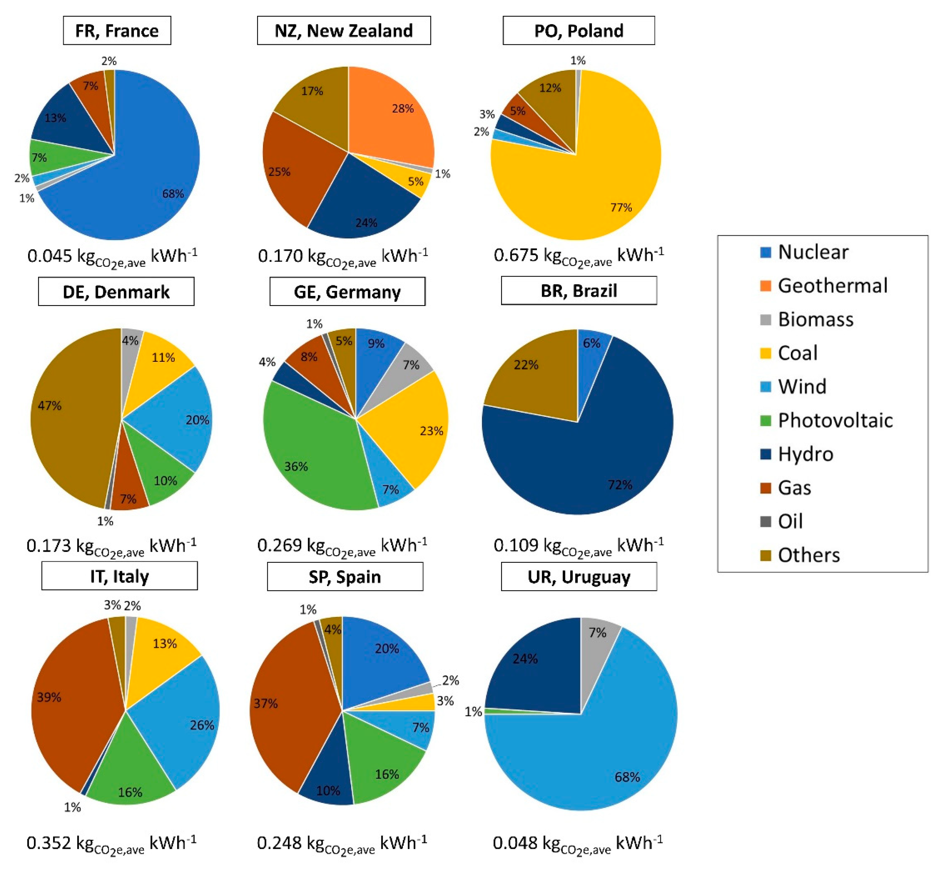
2.1. Representative Energy Scenarios

The optimization of carbon emission was performed considering nine different representative situations based on the fuel mix of the selected countries. Their differences in energy source, share, and hourly variations have been considered to cover the significant number of possible fuel mix situations in the selection process. The average fuel mix of the selected cases is shown in Figure 1. The average carbon intensity of each scenario is also shown in the same figure. Imported energy, among others, are included in the fuel mix within the label “Others”.

The main characteristics of each fuel mix are detailed to understand the hourly carbon intensity values used as input of the optimization problem, as follows:

• France presents the highest share of nuclear energy, but also it is characterized by a high wind energy share that helps to contribute to a notable lower carbon intensity;
• New Zealand electricity origin is similarly distributed in four sources: geothermal, gas, hydro, and “others”, including coal;
• The Polish fuel mix is mainly based on coal-burning based on its abundance in the mines. Renewable and nuclear power is mostly absent in the polish electricity generation system;
• In Denmark, almost half of the electricity is imported from neighboring countries (“others” cover 47% of the fuel mix). The following energy source by relevance is the wind power and then completed by coal, gas and photovoltaic (PV) with comparable influence;
• Germany is the national grid system with a presence of PV energy of all reported. Coal is also an important energy source, whereas the rest of the electricity sources are between 5% and 10%;
• The Brazilian fuel mix is characterized by the higher presence of the hydroelectric power being completed by wind energy and “others”;
• The Italian national grid highlights the significant amount of gas-powered electricity plants, which can be used in a higher efficiency combined cycle plant. A high wind power energy share can be depicted, which is followed by PV and coal;
• The Spanish situation is like that of Italy, with a more significant hydroelectric and nuclear power presence instead of wind and coal.
• Uruguayan electricity production is mainly based on wind energy, and then completed with hydropower energy and finally, biomass.

Countries mainly based on wind energy reduce the carbon footprint emission during nighttime, whereas those with a high share of solar energy, during day hours. Hydropower, geothermal and nuclear power can be considered as constantly available. When the electricity production cannot be covered with the available renewable and nuclear energy plants, fossil fuel (gas, oil and coal) power plants will be needed, being coal the most detrimental to the environment.

The indirect emissions of a refrigeration system are usually calculated by evaluating its energy consumption during standard operating conditions. Then, it is multiplied by an average carbon intensity that depends on the fuel mix of the selected country (see Figure 1 for the values considered). However, this method does not assume that the carbon intensity can vary over a defined time horizon. It is mainly reflected in countries with a higher penetration of RES. Therefore, carbon intensity value varies from hour to hour. Figure 2 depicts the hourly carbon intensity profiles of the investigated countries for a selected day of June (based on data from Tomorrow).

Figure 2 shows countries with noticeable electricity production from RES, such as Germany, Uruguay, Denmark, and Italy. There are other countries, Spain, Brazil, Poland, in which these variations are not evident. A statistical investigation was performed using box plots to characterize the variation of carbon intensity values over the reference day for each country (Figure 3). In Germany, France, New Zealand, and Brazil, carbon intensity values are well-distributed around the median value, but they change in a narrow range, excluding Germany.

The analysis resulting from Figure 3 is fundamental to understand the percentage variation of carbon intensity values over a specified period. Then, the achievement of a carbon emission saving by applying an optimization procedure can be evaluated. In this way, Figure 4 reports the percentage variation distribution of the carbon intensity values referred to as the median value for each investigated country.

In Figure 4, each box-plot included in Figure 3 is represented by its percentage deviation from the median value. This means that the box-plots of Figure 3 were normalized to their median value to have further information about the variability of carbon emission for each country. The following equation was used to evaluate $\%{\Delta }_{CI}$:

$$\%{\Delta }_{CI}=\frac{C{I}_{q,p}-C{I}_{median}}{C{I}_{median}}\ast 100,$$

(1)

where $C{I}_{q,p}$ is the carbon intensity related to the quartile p, and $C{I}_{median}$ is the median value of carbon intensity (i.e., the second quartile).

In Figure 4, those countries with a more significant variation in their carbon intensity over a day (France (FR) and Uruguay (UR)) can be easily identified with a high level of accuracy. In detail, carbon intensity values vary between −38% and +13% for France and between −27% and +95% for Uruguay. Accordingly, carbon emission savings for both scenarios can be expected. Moreover, Germany (GE) and Denmark (DE) also show significant variability of carbon intensities, whereas minor changes can be noticed for the rest of the countries investigated.

2.2. Optimization Problem and Analysis Methodology

The possibility of achieving a carbon emission reduction for a cabinet refrigerator with PCM in some representative scenarios was investigated by solving an optimization problem. The latter was developed considering experimental data [43] used to represent the behavior of the cabinet refrigerator in terms of ON time, OFF time, and average power absorbed by the compressor during the ON time (

Table 1. Experimental data used as inputs for the optimization model [43].

	Δexp (K)	τON (s)	τOFF (s)	P (W)
with PCM	1	1263	9112	215.2
	2	4322	32,337	218.0
	3	6040	48,420	221.9
without PCM	1	233	1653	212.2
	2	638	4923	210.6
	3	1027	8325	210.5

). Refer to Maiorino et al. [43] for further details about the experimental tests.

The objective function is represented by the overall indirect carbon emission of the refrigerator system ($E{M}_H$) over a pre-defined time horizon ($H$). The time horizon is adequately divided into different time steps ($\delta \tau$) to solve the optimization problem. Therefore, the following equation can be considered as representative of the optimization problem:

$$\underset{{\Delta }_iϵ{\Delta }_{\exp }}{\min }E{M}_H={\displaystyle \sum }_{i=1}^{H}C{I}_i\ast P_i\left({\Delta }_i\right)\ast s_i\ast \delta \tau \ast ={\displaystyle \sum }_{i=1}^{H}C{I}_i\ast E{C}_i,$$

(2)

where ${\Delta }_{exp}$ is the set of hysteresis values proposed during the experimental tests (included in Table 1), $C{I}_i$ is the carbon intensity (see Figure 2), $P_i$ is the average power absorbed by the compressor, ${\Delta }_i$ is the value of the hysteresis, $s_i$ is the state of the compressor and $E{C}_i$ is the electric energy absorbed by the compressor. All variables of Equation (2) are referred to as the i-th time step.

According to the selected hysteresis, the cabinet refrigerator was modelled just considering the average power absorbed during its ON time. Indeed, the refrigeration system is represented by the profile of the power absorbed over the pre-defined time horizon of the optimization problem. Assuming that the compressor of the cabinet refrigerator turns on at the start of the time horizon, the power profile of the system is built considering the initial hysteresis scheduling over the time horizon and considering the constraints regarding ON time, OFF time and average power absorbed by the compressor, experimentally measured and shown in Table 1, which depend on the specific value of the hysteresis at each time-step. Therefore, the power profile of the cabinet refrigerator is iteratively built during the optimization process for each possible solution of hysteresis scheduling.

The decision variables of the optimization problem are the values of hysteresis for each time step. In detail, the output of the optimization problem is represented by the optimal hysteresis scheduling that minimizes carbon emission over the pre-defined time horizon, according to the specified constraints related to the working operations of the cabinet refrigerator observed during the experimental tests. These constraints mainly regard the compliance with the experimental ON and OFF time of the refrigerator at the scheduled hysteresis values, which are needed to simulate the behavior of the system in terms of electricity consumption.

The initial condition of the problem, which is the first starting time of the compressor, must be defined as a constraint. Initially, it is set to 0, i.e., the first starting time is at midnight. Then, every hour is simulated to find the initial condition that allows for achieving the optimal solution. The latter investigation should be considered in an actual application where door openings can modify the standard working conditions of the refrigerator assumed in this study (regarding the ON and OFF time of the compressor). For example, determine the optimal time to switch on the compressor again after a door opening (when the carbon intensity is lower).

The detailed description and explanation of the constraints of the optimization problem are presented in Maiorino et al. [44]. To summarize, the carbon intensity profile, the time horizon, the time step, and the average power absorbed by the compressor represent the inputs of the optimization problem and the ON and OFF time of each cycle according to the hysteresis value. As a result, the optimization problem provides the optimal hysteresis scheduling that minimizes carbon emissions and the minimum carbon emissions value over the defined time horizon. The Simulated Annealing (SA) technique is used to solve the optimization problem by a routine programmed in MATLAB. This meta-heuristic technique was used since it is straightforward to code and implement, and it is a well-established technique in the field of optimization problems.

Furthermore, it is faster than other population-based methods, such as Genetic Algorithm (GA) and Particle Swarm Optimization (PSO), and it should lead to the same results since a relatively small solution space characterizes the optimization problem. The SA optimization method uses a stochastic approach to search for and move to new solutions, called neighborhood solutions. These solutions are analogous to the different states of energy during the annealing process of metal. Hence, starting from an initial solution (initial state of energy) at an initial temperature (T₀), a random perturbation is imposed to find a new neighborhood solution (another possible state of energy). Two different arrays of scheduled hysteresis represent the initial and the neighborhood solutions Δs. Then, the difference in the energy between the two solutions (ΔE = E₂ − E₁) is computed. Suppose the energy in the previous state (E₁) is lower than the new one (E₂). In that case, the new solution is accepted according to a probability function that depends on the present temperature (T) of the process. On the other hand, if the energy in the previous state is higher than the new one, the new solution is always accepted. The cost function EM_H represents the energy of each solution. After, the search for new solutions can decrease the temperature according to a defined cooling schedule until the stopping conditions are reached. Stopping conditions can be defined by the final temperature of the process (T_end) or the maximum number of iterations. Different iterations (st) can be performed simultaneously to explore the entire space of solutions for each temperature step. Any functions can represent the cooling schedule as a function of a defined cooling rate (α). In this work, a geometric temperature decrease was applied with a cooling rate of 0.99. The temperatures used in the SA method are dummy variables that simulate the cooling process of annealing metal. The inputs of the algorithm are the carbon intensity profile, the SA parameters (the initial and the final temperature, the cooling rate and the number of iterations per each temperature step), the optimization time horizon and the time-step. The carbon emission, the optimized scheduling of hysteresis values and the profile of the power absorbed by the compressor over the pre-defined time horizon represent the outputs of the entire procedure.

After solving the optimization problem considering the representative scenarios described in Section 2, a post-processing step is performed to analyze the resulting data. In detail, the post-processing analysis aims to investigate the existence of a direct (or indirect) relation between the carbon emission variation obtained with the optimal hysteresis scheduling and the corresponding carbon intensity profile. The carbon intensity profiles by some quantitative statistical indexes can describe the variability of carbon intensity values over the defined time horizon regarding range, dispersion, and positioning. Therefore, four different indexes (standard deviation, range, inter-quartile range (IQR), and Median Absolute Deviation (MAD)) are evaluated for each carbon intensity profile, and each of them is normalized on the average carbon intensity ($C{I}_{ave}$), already shown in Figure 1. All the indexes are calculated as percentage values.

The standard deviation normalized on the average carbon intensity (relative standard deviation ${\sigma }_n$) is calculated as follows:

$$\%{\sigma }_n=\frac{\sigma }{\left|C{I}_{ave}\right|}=\frac{\sqrt{\frac{1}{m-1}{{\displaystyle \sum }}_{k=1}^m{\left(C{I}_k-C{I}_{ave}\right)}^2}}{\left|C{I}_{ave}\right|}\ast 100,$$

(3)

where $m$ is the number of available carbon intensity values and $C{I}_k$ is the k-th carbon intensity value. The normalized range is calculated with Equation (4):

$$\%Rang{e}_n=\frac{C{I}_{max}-C{I}_{min}}{\left|C{I}_{ave}\right|}\ast 100,$$

(4)

where $C{I}_{max}$ and $C{I}_{min}$ represent the maximum and the minimum value of carbon intensity, respectively. Equation (5) is used to evaluate the normalized inter-quartile range (IQR):

$$\%IQ{R}_n=\frac{C{I}_{q,3}-C{I}_{q,1}}{\left|C{I}_{ave}\right|}\ast 100,$$

(5)

where $C{I}_{q,3}$ and $C{I}_{q,1}$ are the upper and the lower quartile, respectively. The difference can be seen in Figure 3, as the distance between the upper and lower bound of each box-plot. The last index describing the carbon intensity profiles statistically is the Median Absolute Deviation (MAD), which is calculated, as shown in Equation (6):

$$\%MA{D}_n=\frac{R{S}_{median}}{\left|C{I}_{ave}\right|}\ast 100=\frac{{(|C{I}_k-C{I}_{median}|)}_{median}}{\left|C{I}_{ave}\right|}\ast 100,$$

(6)

where $RS$ represents the array of residuals, calculated as the difference between each value of carbon intensity $C{I}_k$ and the median $C{I}_{median}$.

Then, the Pearson’s correlation coefficient ($r$) is calculated for each statistical index described above to investigate the connection between the carbon emission variation obtained with the optimal hysteresis scheduling and the corresponding carbon intensity profile, as follows:

$$r=\frac{{{\displaystyle \sum }}_{z=1}^v\left(\Delta E{M}_z-\Delta E{M}_{ave}\right)\left(y_z-y_{ave}\right)}{\sqrt{{{\displaystyle \sum }}_{z=1}^v{\left(\Delta E{M}_z-\Delta E{M}_{ave}\right)}^2{{\displaystyle \sum }}_{z=1}^v{\left(y_z-y_{ave}\right)}^2}},$$

(7)

where $c$ is the number of representative energy scenarios (in this study, it is equal to 9), $\Delta E{M}_z$ is the carbon emission variation of the z-th scenario, $\Delta E{M}_{ave}$ is the average carbon emission variation among all scenarios, $y_z$ is the statistical index calculated for the carbon intensity profile of the z-th scenario and $y_{ave}$ is the average statistical index among all scenarios. The evaluation of Pearson’s correlation coefficient helps understand which of the calculated indexes better the effect of the optimization process on the results.

3. Results and Discussion

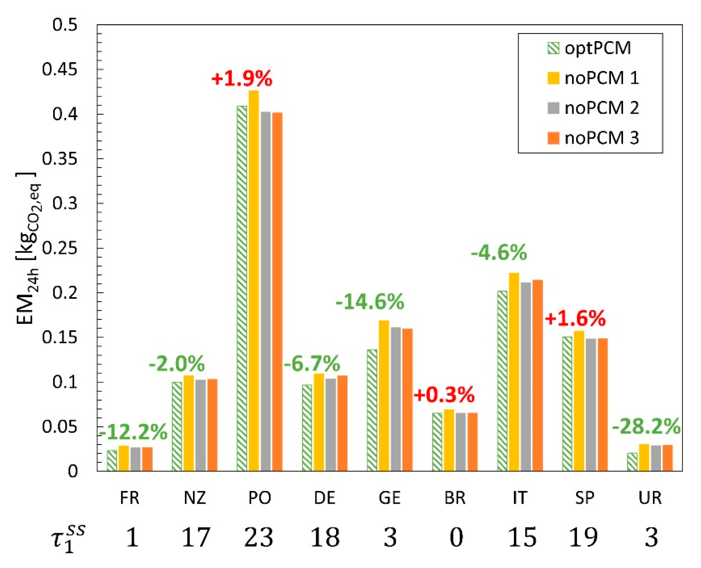
3.1. Daily Carbon Emission Optimization

The carbon emission optimization routine results imposing the initial condition at 0 are shown in Figure 5 for all the representative energy scenarios. The optimal daily carbon emission related to the energy consumption of the refrigerator with PCM (optPCM) is shown and compared with those results of the refrigerator working without PCM at three different hysteresis values (“noPCM 1”, “noPCM 2”, “noPCM 3”). The percentage values above each bar represent the difference between the optimal carbon emission with PCM and the best value obtained simulating the refrigerator without PCM with a fixed hysteresis.

It can be noticed that a carbon emission reduction can be achieved for some representative cases, from −1.9% (Germany, GE) to −19.0% (Uruguay, UR). However, five of the nine representative cases are not positively affected by the optimization process. Despite the optimization of hysteresis scheduling, the introduction of PCM increases from +0.3% (Brazil, BR) to +5.8% (New Zealand, NZ) of the daily carbon emission. A noticeable improvement of the environmental performance of the cabinet refrigerator with PCM is achieved varying the initial condition of the optimization problem, i.e., the initial starting time of the compressor. The effect of the initial condition variation was analyzed, repeating the optimization procedure for each possible initial starting time within the time horizon. The results of the second optimization phase are shown in Figure 6.

It is evidenced that the variation of the first starting time of the compressor (the optimal first starting time of the compressor is shown at the bottom of Figure 6) decreases the daily carbon emissions compared to the previous results (Figure 5) for all the representative case studies. Reducing daily carbon emissions is more pronounced for countries that showed benefits, such as France (from −9.3% to −12.2%) or Germany (from −10.3% to −14.6%). Furthermore, an improvement (carbon emissions reduction) can also be achieved in Italy and New Zealand (−4.6% and −2.0%, respectively), contrary to the previous results (+4.0% and +5.8%, respectively). Therefore, considering the variation of the first starting time of the compressor, daily carbon emissions of the refrigerator system in six of the nine representative countries are reduced. It is caused by a match between the carbon intensity profiles, and the optimized hysteresis scheduling is found.

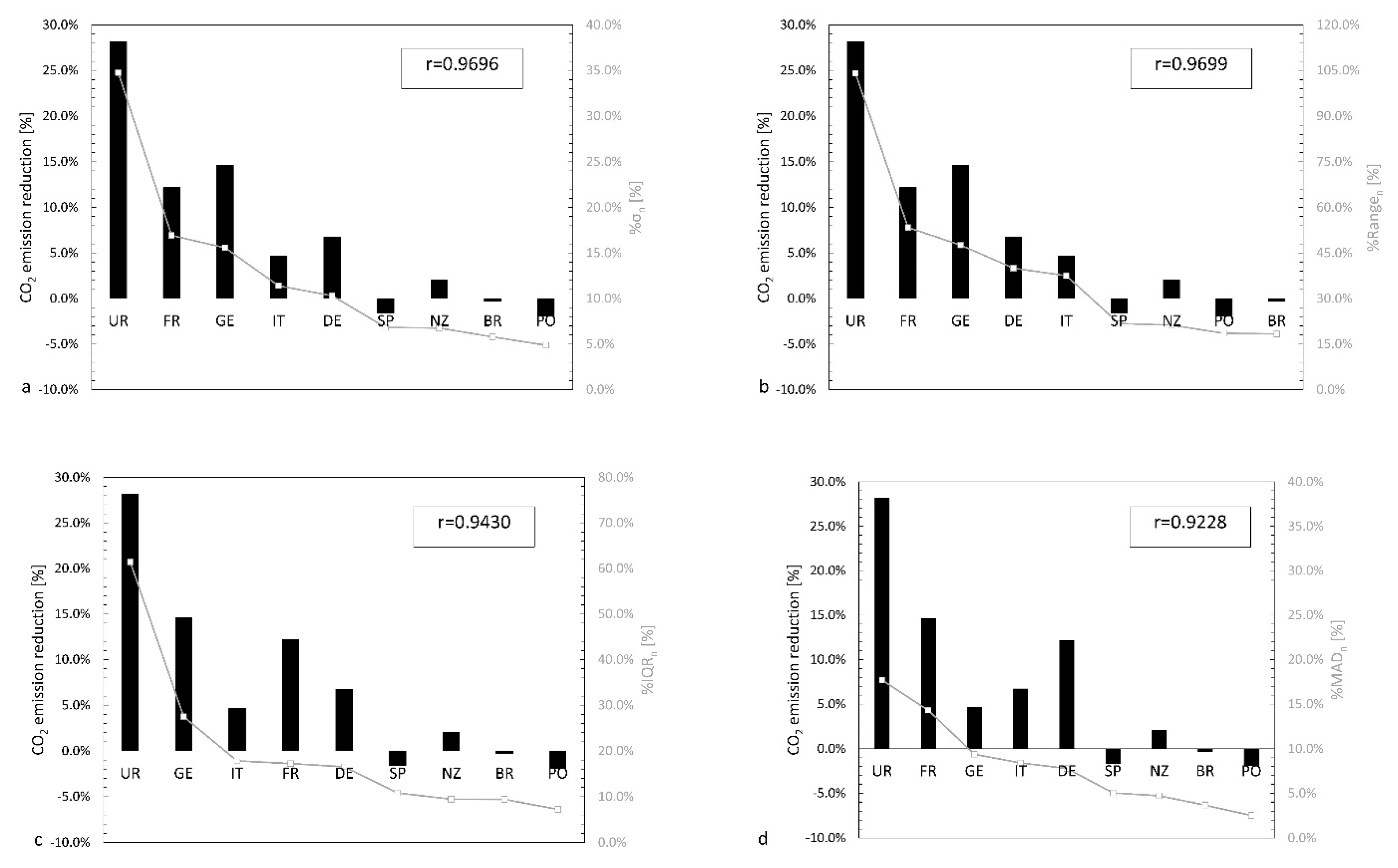
3.2. Statistical Analysis

Figure 7 shows the statistical analysis results needed to identify a correlation between the carbon emission variation obtained by the optimization process and the carbon intensity profile for each representative country. The carbon emission variation is shown on the left y-axis of each plot, whereas on the right y-axis, the statistical index used to describe the carbon intensity profile is displayed. The statistical indexes are calculated using Equations (3)–(6). Furthermore, the correlation degree (r) of each statistical index with the carbon emission variation is reported on each plot.

It can be noticed that all four indexes have a direct correlation with the carbon emission variation. The standard deviation and the range are the best indexes to identify carbon emission reduction possibilities from the carbon intensity profiles. Indeed, their correlations with the carbon intensity variations are 0.9696 and 0.9699, respectively, whereas the correlations of IQR and MAD are 0.9430 (Figure 7c) and 0.9228 (Figure 7d), respectively. Hence, these two indexes can be used to understand if there is a possibility to achieve a carbon emission reduction adopting the optimization of hysteresis scheduling of a cabinet refrigerator incorporating a PCM.

In detail, from Figure 7a,b, one can see that a reduction of the daily carbon intensity can be achieved if the normalized standard deviation (Equation (3)) or the normalized range (Equation (4)) is higher than approximately 10% and 30%, respectively. Only one exception is found, the case of New Zealand, which shows a slight daily carbon emission reduction despite a normalized standard deviation of less than 10% and a normalized range less than 30% of its carbon intensity profile. This may be due to many factors that affect the carbon intensity profiles not considered in this analysis. Both statistical indexes can be used to perform a preliminary investigation about the carbon emission reduction paying attention to the carbon intensity profile of the country or region of interest. It is strongly suggested to perform a simulation with the optimization routine to ensure the actual possibility of carbon emission saving.

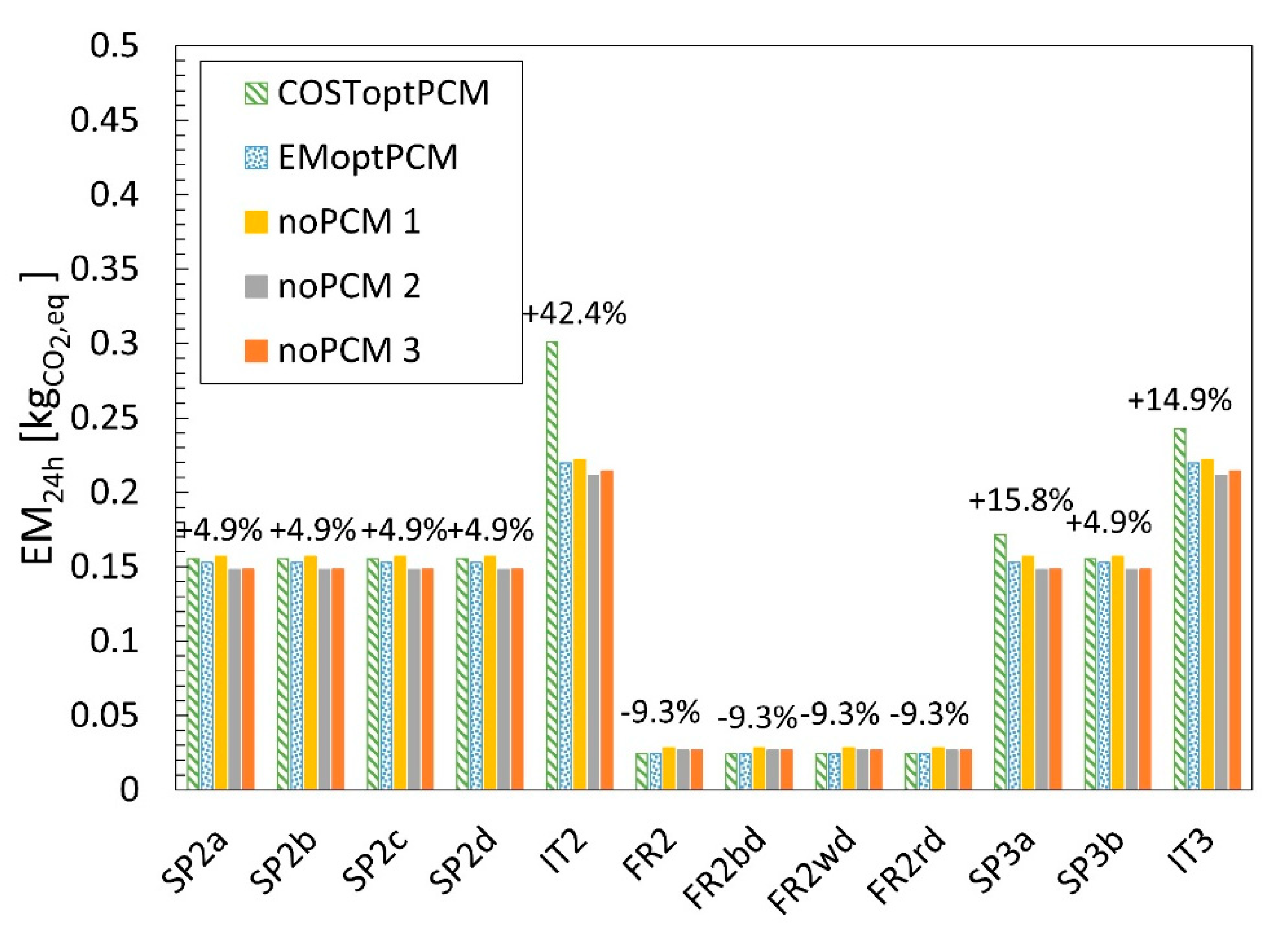
3.3. Comparison with Cost-Optimized Operations

The analysis of the scheduling optimization of a cabinet refrigerator incorporating a PCM is concluded by analyzing the carbon emission optimization solutions from an economic point of view. Then, the cost-optimized solutions found in Maiorino et al. [44] are investigated considering their effect on carbon emission.

The daily running costs of the cabinet refrigerator without PCM and different fixed hysteresis (noPCM 1, noPCM 2 and noPCM3) are shown in Figure 8. This figure contains the cabinet refrigerator results with PCM working with a cost-optimized hysteresis scheduling (COSToptPCM) and working with a hysteresis scheduling optimizing daily carbon emission (EMoptPCM). In the latter case, the initial starting time was also optimized. The percentage values above each bar represent the difference between the daily running cost calculated with a hysteresis scheduling which optimizes daily carbon emission, and the minimum daily running cost obtained simulating the refrigerator without PCM with a fixed hysteresis. For further information about the labels on the x-axis, refer to Maiorino et al. [44].

In general, it can be noticed that optimizing the daily carbon emission leads to an increase in the daily running cost of the refrigerator (up to +9.0%), at least considering 2-TOU tariffs in Spain and Italy. On the contrary, the optimization of carbon emission in France allows achieving also daily running cost savings. In detail, in the latter case, the daily carbon emission optimization leads to the same daily running cost savings shown in Maiorino et al. [44]. The last is because both optimization methods find the exact solution in terms of optimal hysteresis scheduling. Considering 3-TOU tariffs, daily running cost savings can also be achieved by optimizing daily carbon emission in Spain. Still, these savings (0.3% and 2.9% for SP3a and SP3b, respectively) are reduced compared to those that stem from the optimization of daily running cost shown in Maiorino et al. [44] (20.8% and 5.0% for SP3a and SP3b, respectively). The results of the Italian 3-TOU tariff are similar to the 2-TOU tariff, increasing the daily running cost optimizing carbon emission.

Finally, the effect of the running cost optimization on the daily carbon emission is analyzed. The cost-optimized hysteresis scheduling shown in Maiorino et al. [44] is used for feeding the simulation of the refrigerator with PCM. The results of the simulations for Spain, Italy and France are shown in Figure 9.

It is worth noting that, in France, the daily carbon emission variation of the refrigerator with cost-optimized scheduling is the same that obtained with the optimization of the daily carbon emission (−9.3%, see Figure 5). The latter confirms that the same hysteresis scheduling can lead to both economic and environmental benefits. For the rest of the studies, the cost optimization of the hysteresis scheduling involves a noticeable increase in the daily carbon emission (up to +42.4% for the 2-TOU Italian tariff, IT2).

The case studies showed that a simultaneous economic and environmental benefit (excluding some cases) is not possible, and therefore, a trade-off between them is required. However, if the objective is a cost-saving or carbon emission reduction, the scheduling of a cabinet refrigerator incorporating a PCM can be optimized, even if the energy consumption of the refrigerator with PCM is initially higher.

4. Conclusions

Cold production systems combined with thermal energy storage offers an exciting possibility to switch the electric energy consumption to more favorable periods. Usually, optimization for refrigeration and air conditioning systems is performed based on economic terms. However, environmental concepts should be considered in smart controlled systems, given the current climate urgency. This paper proposes using an algorithm control in a cabinet refrigerator with PCM to minimize the carbon emissions operating in hours in which the carbon emission factor is lower. Nine representative carbon intensity profiles have been considered to analyze the possibility of achieving daily carbon emission reduction (France, New Zealand, Poland, Denmark, Germany, Brazil, Italy, Spain, and Uruguay). A statistical analysis has been performed to identify a correlation between daily carbon emission variations and carbon intensity profiles. Finally, environmentally optimized results have been compared with those regarding the cost-optimized operations shown in a previous work.

The optimization produces a carbon emission reduction for countries with a significant hourly carbon intensity variation, from −1.9% (Germany) to −19.0% (Uruguay) but increases for the contrary situation, from +0.3% (Brazil) to +5.8% (New Zealand). However, it was noticed that the carbon emission reduction strongly depends on the first starting time of the refrigerator considered. The selection of the most valuable first starting time reduces the carbon emission for all cases. Italy and New Zealand can move from a situation with a deterioration of the results (−4.6% and −2.0%, respectively) to a clear benefit (+4.0% and +5.8%, respectively). Besides, the reduction is more visible for countries that already showed benefits, such as France (from −9.3% to −12.2%) or Germany (from −10.3% to −14.6%)

The best statistical indexes to correlate the carbon intensity variation with the carbon emission reduction in the refrigerator with PCM with optimized operations are the normalized standard deviation and the normalized range, with r of 0.9696 and 0.9699, whereas the correlations for inter-quartile range and median absolute deviation resulted in 0.9430 and 0.9228. For most cases, the daily carbon emission can be reduced if the normalized standard deviation or the normalized range is higher than approximately 10% and 30%, respectively, except for New Zealand.

Optimizing the daily carbon emission does not necessarily imply a decrease in the daily running cost savings compared to the not-optimized situation. The daily carbon emission optimization can increase the running cost up to 9% or reduce it to 2.9%. The result depends strongly on the tariffs and the carbon emission profile. The same situation happens on the contrary, considering the daily carbon emission of the refrigerator with cost-optimized scheduling, in which an increase of up to 42.4% has been found. Therefore, results demonstrate that attending to the reported carbon emission profiles, the optimization of both parameters simultaneously is not possible with the current electricity time-based tariffs, and a trade-off is required. An alternative would be the improvement of the relation between the hourly tariff and the carbon emission factor.

References

1. United Nations Paris Climate Change Conference-November 2015, COP 21. In Proceedings of the Adoption of The Paris Agreement, Paris, France, 30 November–11 December 2015; 2015. Available online: https://unfccc.int/resource/docs/2015/cop21/eng/l09r01.pdf (accessed on 9 April 2021).
2. IEA. Global Energy and CO2 Status Report 2018. The Latest Trends in Energy and Emissions in 2018; IEA: Paris, France, 2019. [Google Scholar]
3. IPCC. Climate Change 2014: Mitigation of Climate Change. Contribution of Working Group III to the Fifth Assessment Report of the Intergovernmental Panel on Climate Change, AR5 ed.; Edenhofer, O., Pichs-Madruga, R., Sokona, Y., Farahani, E., Kadner, S., Seyboth, K., Adler, A., Baum, I., Brunner, S., Eickemeier, P., et al., Eds.; Cambridge University Press: Cambridge, UK; New York, NY, USA, 2014. [Google Scholar]
4. Gielen, D.; Boshell, F.; Saygin, D.; Bazilian, M.D.; Wagner, N.; Gorini, R. The role of renewable energy in the global energy transformation. Energy Strateg. Rev. 2019, 24, 38–50. [Google Scholar] [CrossRef]
5. Winkler, J.; Gaio, A.; Pfluger, B.; Ragwitz, M. Impact of renewables on electricity markets—Do support schemes matter? Energy Policy 2016, 93, 157–167. [Google Scholar] [CrossRef]
6. Braeuer, F.; Rominger, J.; McKenna, R.; Fichtner, W. Battery storage systems: An economic model-based analysis of parallel revenue streams and general implications for industry. Appl. Energy 2019, 239, 1424–1440. [Google Scholar] [CrossRef]
7. Winkler, J.; Pudlik, M.; Ragwitz, M.; Pfluger, B. The market value of renewable electricity—Which factors really matter? Appl. Energy 2016, 184, 464–481. [Google Scholar] [CrossRef]
8. Pursiheimo, E.; Holttinen, H.; Koljonen, T. Inter-sectoral effects of high renewable energy share in global energy system. Renew. Energy 2019. [Google Scholar] [CrossRef]
9. Mosquera-López, S.; Nursimulu, A. Drivers of electricity price dynamics: Comparative analysis of spot and futures markets. Energy Policy 2019, 126, 76–87. [Google Scholar] [CrossRef]
10. Zipp, A. The marketability of variable renewable energy in liberalized electricity markets—An empirical analysis. Renew. Energy 2017, 113, 1111–1121. [Google Scholar] [CrossRef]
11. Kyritsis, E.; Andersson, J.; Serletis, A. Electricity prices, large-scale renewable integration, and policy implications. Energy Policy 2017, 101, 550–560. [Google Scholar] [CrossRef] [Green Version]
12. Paraschiv, F.; Erni, D.; Pietsch, R. The impact of renewable energies on EEX day-ahead electricity prices. Energy Policy 2014, 73, 196–210. [Google Scholar] [CrossRef] [Green Version]
13. Eid, C.; Koliou, E.; Valles, M.; Reneses, J.; Hakvoort, R. Time-based pricing and electricity demand response: Existing barriers and next steps. Util. Policy 2016, 40, 15–25. [Google Scholar] [CrossRef] [Green Version]
14. Hansen, K.; Breyer, C.; Lund, H. Status and perspectives on 100% renewable energy systems. Energy 2019, 175, 471–480. [Google Scholar] [CrossRef]
15. Hu, M.; Xiao, F.; Jørgensen, J.B.; Wang, S. Frequency control of air conditioners in response to real-time dynamic electricity prices in smart grids. Appl. Energy 2019, 242, 92–106. [Google Scholar] [CrossRef]
16. Schné, T.; Jaskó, S.; Simon, G. Embeddable adaptive model predictive refrigerator control for cost-efficient and sustainable operation. J. Clean. Prod. 2018, 190, 496–507. [Google Scholar] [CrossRef]
17. Nakabi, T.A.; Toivanen, P. An ANN-based model for learning individual customer behavior in response to electricity prices. Sustain. Energy Grids Netw. 2019, 18, 100212. [Google Scholar] [CrossRef]
18. Yalcintas, M.; Hagen, W.T.; Kaya, A. Time-based electricity pricing for large-volume customers: A comparison of two buildings under tariff alternatives. Util. Policy 2015, 37, 58–68. [Google Scholar] [CrossRef]
19. Cohen, F.; Glachant, M.; Söderberg, M. The impact of energy prices on product innovation: Evidence from the UK refrigerator market. Energy Econ. 2017, 68, 81–88. [Google Scholar] [CrossRef] [Green Version]
20. Niro, G.; Salles, D.; Alcântara, M.V.P.; da Silva, L.C.P. Large-scale control of domestic refrigerators for demand peak reduction in distribution systems. Electr. Power Syst. Res. 2013, 100, 34–42. [Google Scholar] [CrossRef]
21. Zehir, M.A.; Bagriyanik, M. Demand Side Management by controlling refrigerators and its effects on consumers. Energy Convers. Manag. 2012, 64, 238–244. [Google Scholar] [CrossRef]
22. Bálint, R.; Fodor, A.; Hangos, K.M.; Magyar, A. Cost-optimal model predictive scheduling of freezers. Control Eng. Pract. 2018, 80, 61–69. [Google Scholar] [CrossRef] [Green Version]
23. Mohammad, N.; Rahman, A. Transactive control of industrial heating-ventilation-air-conditioning units in cold-storage warehouses for demand response. Sustain. Energy Grids Netw. 2019, 18, 100201. [Google Scholar] [CrossRef]
24. Hu, M.; Xiao, F.; Jørgensen, J.B.; Li, R. Price-responsive model predictive control of floor heating systems for demand response using building thermal mass. Appl. Therm. Eng. 2019, 153, 316–329. [Google Scholar] [CrossRef]
25. Biyik, E.; Kahraman, A. A predictive control strategy for optimal management of peak load, thermal comfort, energy storage and renewables in multi-zone buildings. J. Build. Eng. 2019, 25, 100826. [Google Scholar] [CrossRef]
26. Tabares-Velasco, P.C.; Speake, A.; Harris, M.; Newman, A.; Vincent, T.; Lanahan, M. A modeling framework for optimization-based control of a residential building thermostat for time-of-use pricing. Appl. Energy 2019, 242, 1346–1357. [Google Scholar] [CrossRef]
27. Ringkjøb, H.-K.; Haugan, P.M.; Solbrekke, I.M. A review of modelling tools for energy and electricity systems with large shares of variable renewables. Renew. Sustain. Energy Rev. 2018, 96, 440–459. [Google Scholar] [CrossRef]
28. Azhgaliyeva, D. Energy Storage and Renewable Energy Deployment: Empirical Evidence from OECD countries. Energy Procedia 2019, 158, 3647–3651. [Google Scholar] [CrossRef]
29. Gang, W.; Wang, S.; Xiao, F.; Gao, D. District cooling systems: Technology integration, system optimization, challenges and opportunities for applications. Renew. Sustain. Energy Rev. 2016, 53, 253–264. [Google Scholar] [CrossRef]
30. Li, Y.; Rezgui, Y.; Zhu, H. District heating and cooling optimization and enhancement—Towards integration of renewables, storage and smart grid. Renew. Sustain. Energy Rev. 2017, 72, 281–294. [Google Scholar] [CrossRef]
31. Child, M.; Kemfert, C.; Bogdanov, D.; Breyer, C. Flexible electricity generation, grid exchange and storage for the transition to a 100% renewable energy system in Europe. Renew. Energy 2019, 139, 80–101. [Google Scholar] [CrossRef]
32. Dostál, Z.; Ladányi, L. Demands on energy storage for renewable power sources. J. Energy Storage 2018, 18, 250–255. [Google Scholar] [CrossRef]
33. Paiho, S.; Saastamoinen, H.; Hakkarainen, E.; Similä, L.; Pasonen, R.; Ikäheimo, J.; Rämä, M.; Tuovinen, M.; Horsmanheimo, S. Increasing flexibility of Finnish energy systems—A review of potential technologies and means. Sustain. Cities Soc. 2018, 43, 509–523. [Google Scholar] [CrossRef]
34. She, X.; Cong, L.; Nie, B.; Leng, G.; Peng, H.; Chen, Y.; Zhang, X.; Wen, T.; Yang, H.; Luo, Y. Energy-efficient and -economic technologies for air conditioning with vapor compression refrigeration: A comprehensive review. Appl. Energy 2018, 232, 157–186. [Google Scholar] [CrossRef]
35. Nazir, H.; Batool, M.; Bolivar Osorio, F.J.; Isaza-Ruiz, M.; Xu, X.; Vignarooban, K.; Phelan, P.; Inamuddin; Kannan, A.M. Recent developments in phase change materials for energy storage applications: A review. Int. J. Heat Mass Transf. 2019, 129, 491–523. [Google Scholar] [CrossRef]
36. Zhou, E.; Cole, W.; Frew, B. Valuing variable renewable energy for peak demand requirements. Energy 2018, 165, 499–511. [Google Scholar] [CrossRef]
37. Mastani Joybari, M.; Haghighat, F.; Moffat, J.; Sra, P. Heat and cold storage using phase change materials in domestic refrigeration systems: The state-of-the-art review. Energy Build. 2015, 106, 111–124. [Google Scholar] [CrossRef]
38. Killian, M.; Kozek, M. Ten questions concerning model predictive control for energy efficient buildings. Build. Environ. 2016, 105, 403–412. [Google Scholar] [CrossRef]
39. Pertzborn, A. Using distributed agents to optimize thermal energy storage. J. Energy Storage 2019, 23, 89–97. [Google Scholar] [CrossRef]
40. Kamal, R.; Moloney, F.; Wickramaratne, C.; Narasimhan, A.; Goswami, D.Y. Strategic control and cost optimization of thermal energy storage in buildings using EnergyPlus. Appl. Energy 2019, 246, 77–90. [Google Scholar] [CrossRef]
41. Bista, S.; Hosseini, S.E.; Owens, E.; Phillips, G. Performance improvement and energy consumption reduction in refrigeration systems using phase change material (PCM). Appl. Therm. Eng. 2018, 142, 723–735. [Google Scholar] [CrossRef]
42. Yusufoglu, Y.; Apaydin, T.; Yilmaz, S.; Paksoy, H.O. Improving performance of household refrigerators by incorporating phase change materials. Int. J. Refrig. 2015, 57, 173–185. [Google Scholar] [CrossRef]
43. Maiorino, A.; Del Duca, M.G.; Mota-Babiloni, A.; Greco, A.; Aprea, C. The thermal performances of a refrigerator incorporating a phase change material. Int. J. Refrig. 2019, 100, 255–264. [Google Scholar] [CrossRef]
44. Maiorino, A.; Del Duca, M.G.; Mota-Babiloni, A.; Aprea, C. Achieving a running cost saving with a cabinet refrigerator incorporating a phase change material by the scheduling optimisation of its cyclic operations. Int. J. Refrig. 2020, 117, 237–246. [Google Scholar] [CrossRef]
45. Tomorrow, ElectricityMap. (n.d.). Available online: https://www.electricitymap.org/zone (accessed on 6 June 2019).
Figure 1. Fuel mix and average carbon intensity for different countries (based on data from Tomorrow [45]).
Energies 14 02154 g001
Figure 2. Hourly carbon intensity profiles for different countries during a day of June (based on data from Tomorrow [45]).
Energies 14 02154 g002
Figure 3. Box-plots of carbon intensities for different countries (based on data from Tomorrow [45]).
Energies 14 02154 g003
Figure 4. Relative variation of carbon intensity values compared to the median value for different countries (based on data from Tomorrow [45]).
Energies 14 02154 g004
Figure 5. Comparison of carbon emission of the refrigerator with and without Phase Change Materials (PCMs) among different case studies with the initial condition equal to 0 (the first starting time of the refrigerator in the optimization procedure was fixed at 0). The percentage values above each bar represent the difference between the optimal hysteresis scheduling, optimizing daily carbon emission. The minimum daily carbon emission obtained simulates the refrigerator without PCM with a fixed hysteresis.
Energies 14 02154 g005
Figure 6. Comparison of carbon emission of the refrigerator with and without PCM among different case studies with the best initial condition. The percentage values above each bar represent the difference between the optimal hysteresis scheduling, optimizing daily carbon emission. The minimum daily carbon emission obtained simulates the refrigerator without PCM with a fixed hysteresis.
Energies 14 02154 g006
Figure 7. Relations between carbon emission reduction and statistical indexes related to the carbon intensity profiles: (a) standard deviation, (b) range, (c) Inter-Quartile Range, and (d) Median Absolute Deviation.
Energies 14 02154 g007
Figure 8. Daily running cost of the cabinet refrigerator working with scheduled hysteresis obtained by carbon emission optimization for the cases studies considered in Maiorino et al. [44]. The percentage values above each bar represent the difference between the daily running cost calculated with a hysteresis scheduling which optimizes daily carbon emission, and the minimum daily running cost obtained simulating the refrigerator without PCM with a fixed hysteresis.
Energies 14 02154 g008
Figure 9. Daily carbon emission of the cabinet refrigerator working with the scheduled hysteresis obtained by the running cost optimization performed in Maiorino et al. [44]. The percentage values above each bar represent the difference between the carbon emission calculated with a hysteresis scheduling which optimizes daily running cost, and the minimum carbon emission obtained simulating the refrigerator without PCM with a fixed hysteresis.
Energies 14 02154 g009