Article

High-Frequency Sea-Level Cycle Reconstruction and Vertical Distribution of Carbonate Ramp Shoal Facies Dolomite Reservoir in Gucheng Area, East Tarim Basin

1
College of Energy, Chengdu University of Technology, Chengdu 610059, China
2
Exploration and Development Research Institute, Daqing Oilfield Company Ltd., Daqing 163712, China
3
Research Branch of Daqing Oilfield, Key Laboratory of Carbonate Reservoirs, CNPC, Daqing 163712, China
4
Petro China Hangzhou Research Institute of Geology, Hangzhou 310023, China
5
Key Laboratory of Carbonate Reservoirs, CNPC, Hangzhou 310023, China
6
College of Geosciences, China University of Petroleum (Beijing), Beijing 102249, China
7
School of Earth Sciences, Northeast Petroleum University, Daqing 163318, China
*
Authors to whom correspondence should be addressed.
Energies 2022, 15(12), 4287; https://doi.org/10.3390/en15124287
Submission received: 8 April 2022 / Revised: 22 May 2022 / Accepted: 6 June 2022 / Published: 11 June 2022

Abstract

:
During the sedimentary period of the Ordovician Yingshan Formation, the carbonate platform of the Gucheng area in the Tarim basin was characterized by a distally steepened ramp. Relative sea-level changes exerted a strong influence on the shoal facie dolomite reservoirs of the 3rd Member of the Ordovician Yingshan Formation (the Ying 3 member), sedimented in the context of a shallow water environment on the carbonate ramp. However, previous studies that lacked high-frequency sea-level changes in the Gucheng area prevent further dolomite reservoir characterization. The current work carries out systematic sampling based on the continuous core from the upper and middle parts of the Ying 3 member in two newly drilled exploration wells (GC17 and GC601) and a series of geochemistry analyses, such as C-O isotope, Sr isotope, and rare earth elements (REE), which helps to investigate the features of the shoal facies dolomite reservoir development against high-frequency sea-level changes. With the help of Fischer plots of these two wells, high-density δ13C data (sample interval is about 0.272 m) were merged to construct a comprehensive curve, contributing to characterizing the high-frequency sea-level changes of the upper and middle parts of the Ying 3 member in the Gucheng area and validating the relationship between the pore-vug vertical distribution and high-frequency sea-level changes. Results revealed that the porosity of dolomite reservoirs increased when the high-frequency sea-level fell and decreased when it rose. Furthermore, the karst surface can be found at the top of the upward-shallowing cycle during the high-frequency sea-level falling; the pore-vug reservoirs are concentrated below the karst exposure surface, and porous spaces are more developed closer to the top of the cycle. The high frequency sea-level curve built in this study can be used as a standard for further research of regional sea-levels in the Gucheng area, and this understanding is highly practical in the prediction of shoal facies carbonate reservoir in carbonate ramp.

1. Introduction

Studies on paleo-relative sea-level changes are widely applied in many fields, such as carbonate sedimentology, paleoenvironment reconstruction, and hydrocarbon exploration [1,2,3]. In general, relative sea-level changes dominate the carbonate platform margin type and the structure of carbonate sediments [4]; these sediments thus record that information in their sedimentation, allowing researchers to study paleo-relative sea-level changes despite a lack of direct access to its measurement [1]. The most extensively used methods are as follows: sequence stratigraphy and sediment structure oriented [5,6,7,8], geochemistry oriented [9,10], natural gamma-ray spectral logging oriented [11,12,13,14], and Fischer plot oriented [6,15,16]. It is clear that the cycle order of relative sea-level changes varies since each method allows for individual scale, data density, and time-space resolution. Moreover, the conception of higher sea-level cycle orders requires more continuous data with better time-space resolution. In other words, characterizing the 4th and above order, especially to high-frequency sea-level cycles [17] in a region, must be based on obtaining high-frequency, high-continuity data. The methods in the previous studies mentioned above all have certain drawbacks when used alone. For example, although the seismic data used in the study of sequence stratigraphy have good lateral continuity, the vertical resolution is insufficient. Geochemical analysis requires a large amount of continuous data. It is relatively easy to sample outcrops in the field [18], but in underground hydrocarbon exploration, a continuous core is very precious and the cost is very high. Although the vertical resolution of the logging curve is high, it is necessary to analyze the sensitivity to reduce ambiguity. Thus, a combination of multiple methods seems sensible to pursue a better outcome.
With the deepening of China’s marine carbonate hydrocarbon exploration, breakthroughs in shoal facies dolomite reservoirs inspired researchers, including the Deyang-Anyue area in the Sichuan basin and the Gucheng area in the Tarim basin [19,20,21,22,23]. These exploration examples demonstrate a strong link between the shoal facies dolomite reservoirs and the distribution of shoal facies carbonate sediments under the control of sea-level changes [22]. Relative sea-level changes influenced the productivity and type of carbonate by controlling sedimentary patterns and water energy changes and further influenced the sequence structures of carbonate rocks [24]. For the carbonate ramp, shoal facies dolomite reservoirs cover a broader range with greater gross thickness [25], owing to their long-distance migration along the shoreline and the swing of the high hydrodynamic energy zone; however, high-frequency relative sea-level changes produce more frequent facies migration, because of their gentle declivity and absence of barriers [5,26], which makes the stacking of thin shoal facies dolomite reservoirs more complex [27]. It can even show a mosaic-like distribution pattern lacking clear and regular trends in facies-to-facies transitions [18].
The 3rd member of the Ordovician Yingshan Formation (the Ying 3 member) in the Gucheng area of the Tarim basin witnesses considerable cycled thin intervals in pore-vug beds of its shoal facies dolomite reservoirs, and karst exposure surfaces as well, which indicates a strong relationship with high frequent sea-level changes. However, the restriction of incomplete coring formation and low sampling density in the existing exploration wells leaves studies on paleo-relative sea-level changes crude, let alone high-frequent sea-level changes, preventing further fine correlation and description. Therefore, the current work carries out a systematic sampling, based on the continuous core from the upper and middle parts of the Ying 3 member in two newly drilled exploration wells (GC17 and GC601), and a series of geochemistry analyses, such as the C-O isotope, Sr isotope, and rare earth elements (REE), which helps to investigate the features of the shoal facies dolomite reservoir development in the context of high-frequency sea-level changes. With the help of Fischer plots of these two wells, high-density δ13C data contribute to characterizing high-frequency sea-level changes of the upper and middle parts of the Ying 3 member in the Gucheng area and validating the relationship between vertical pore-vug distribution and high-frequency sea-level changes. The current work fills the blank of the high-frequency sea-level cycle in the Ying 3 member of the Gucheng area. The high frequency sea-level curve built in this study can be used as a standard for further research of regional sea-levels in this area, which is also highly practical in the prediction of shoal facies carbonate reservoir in carbonate ramps.

2. Geological Background

The Gucheng area is situated in the mid-south of the North Depression in the Tarim Basin, on the slope of the Tazhong uplift [28]. It is a second-order structural unit located on the southeast margin of the West Tarim platform [29], adjacent to the Manxi low bulge in the north, and to the Tadong uplift to the east [30,31]. The top surface of the Ordovician carbonate rocks in the target area is structurally a large-wide nose-like uplift inclining toward the northwest, cut by NE faults into several fault blocks with grabens alternating with horsts [28] (Figure 1a).
In the weak extensional tectonic setting of the Cambrian–Early Ordovician period [32], carbonate platforms developed widely in the Gucheng area with a general rise in sea-level. The seismic response showed that the platform style was a distally steepened ramp in the period of the Yingshan Formation [33,34]. Additionally, practice experience of the shoal facies reservoirs shows that the Ordovician Yingshan Formation in this area developed an extensive inner platform shoal and marginal shoal composed of dolomites. Among them, the lower Yingshan Formation (including the Ying 3 member) was dominated by fine- to medium-crystal dolomite with residual granular structures, which were considered favorable reservoir rocks, while the upper Yingshan Formation by calcarenite and dolomite grainstones [28] is a lower quality reservoir than the lower Yingshan Formation (Figure 1b).
After the extensive analysis of lithofacies, several distinct microfacies were found, namely sand shoals (Figure 2a,b), dolomitized shoals (Figure 2c,d), inter-shoal marine (Figure 2e,f), and tidal flat (Figure 2g,h). Moreover, sedimentary structures, such as cross bedding (Figure 2c,d), karstic mosaic (Figure 2i), and seepage silt (Figure 2j), are common in dolomitized shoals, indicating the hydrodynamic environment, during the depositional period, generally featured relatively high-energy turbulence. When it comes to cathodoluminescence analysis, the fine-medium crystalline dolomite of dolomitized shoals is generally the most common in dim, or tan light, and brown light under the cathode rays (Figure 2k,l). This indicates that shoal facie dolomite is mainly affected by the burial process and may be partially transformed by late hydrothermal fluids.

3. Materials and Methods

3.1. Experimental Materials and Methods

GC17 and GC601, two exploration wells, were drilled in Guchengarea within the last 5 years, which have collected over 150 m of continuous core in the Ying 3 member, lower Ordovician, as well as wire logging data, such as GR logging, natural gamma-ray spectral logging, and resistivity logging. In this study, oxygen and carbon stable isotope analysis was performed on 547 dolomite and limestone wall rock samples taken from core and sidewall coring at an average sampling interval of about 0.272 m, with the average data density reaching about 3.68 per meter. Among these samples, 52 were tested by hole rock element analysis and rear earth element (REE) analysis, and 85 were analyzed by the strontium isotope. Two batches of these geochemistry experiments were carried out in different laboratories: the Key Laboratory of Carbonate Reservoirs, CNPC, and the Experiment Center of Exploration and Development Research Institute of Daqing Oilfield. At the same time, the porosity test data of 679 carbonate rock samples in the Ying 3 Member of these two wells were collected.
The oxygen and carbon stable isotope values adopted the Vienna Peedee Belemnite standard (VPDB). Carbonate powders were reacted with 100% phosphoric acid for 4 h at 25 °C for calcite and at 50 °C for dolomite, and the resultant CO2 was measured to determine its oxygen and carbon isotopic ratios using a Delta V advantage + Gasbench mass spectrometer. The reproducibility values of the isotopic measurement for both carbon and oxygen isotopes were better than ±0.01%.
The REE analysis method and process follow the general method of inductively coupled plasma mass spectrometry (ICP-MS) with an Element XR inductively coupled plasma mass spectrometry instrument, whose limit of detection is 10−12, and the measurement error can be regulated to within 5%, meeting the measurement accuracy standards. Selected samples are then crushed to 75 μm in the agate mortar and put into paper sample bags for later use. Acetic acid and nitric acid are used to dissolve and purify, and scaling solution is added to fix the volume to 10 mL. Then, the sample well is shaken for the final instrument test.
The 87Sr/86Sr isotope ratios are tested for selected matrix dolomite and dolomite cements using a Neptune Plus mass spectrometer (MC-ICP-MS). The test temperature was 20 °C, the humidity was 40% RH, the single band was Ta band, and the ionization temperature was 1450 °C The analytical precision of the individual runs is determined to be 0.00005 (2σ). The 87Sr/86Sr of the instrument test standard NBS987 is 0.710244 ± 0.000004. The mean standard error of the mass spectrometer performance was ±0.00003, which conforms to the Chinese national standard GB/T 17672-1999.

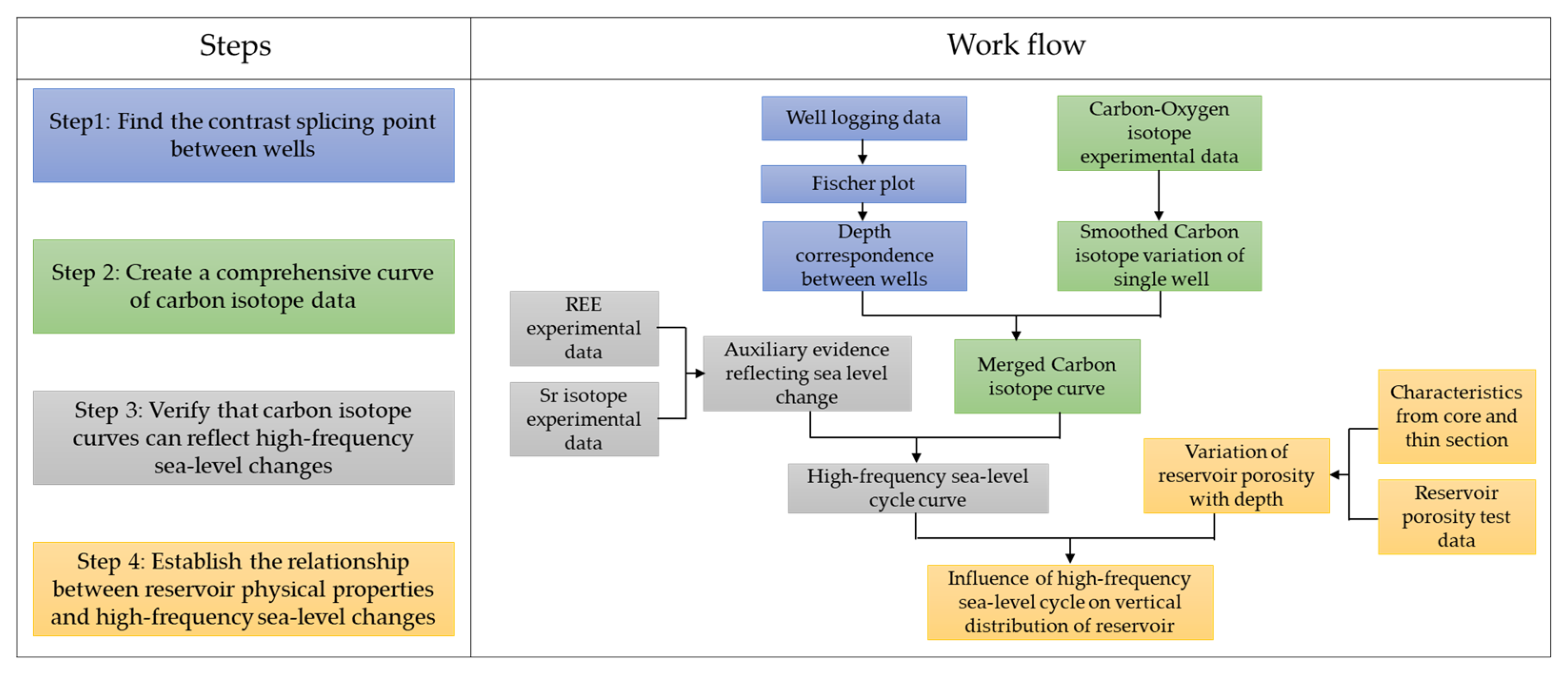
3.2. High-Frequency Sea-Level Curve Reconstruction Methods

In the study of paleo-relative sea-level changes, the oxygen and carbon stable isotopes set a solid foundation for capturing information on sea-level fluctuation [1,9,35,36], with δ13C having been widely applied [36,37], whose principle lies in the fact that the increase of δ13C in carbonate rocks usually relates to the grown biological productivity or the deepened burial of organic matter when the relative sea-level rises. Therefore, there is a positive correlation between δ13C and the relative sea-level in geological history—specifically, δ13C increases when the sea-level climbs up and declines when it drops [38,39,40,41]. Given this, the carbon isotope data of Wells GC601 and GC17 were used to characterize the high-frequency sea-level cycles of the Ying 3 Member in the target region. In order to exploit the collected data of Wells GC17 and GC601 as fully as possible, and to develop a more complete pattern of sea-level changes, we managed to merge the data vertically and get a comprehensive curve on the following conditions:
First, the consistent features that are correlative between Wells GC17 and GC601 must be recognized, which helps to identify the depth correlation between these two wells that can be mapped to a vertical axis. However, it is hardly possible to directly apply lithologic characteristics and well-logging features to finish the stratigraphic correlation. The Fischer plot is thus introduced in this study to assist the task. It is a semi-quantitative graphic of sea-level changes drawn by cumulative departure from mean cycle thickness (CMDT) proposed by Fischer in 1964 [42,43]. After further improvement by Sadler et al. [44] and Day [45], this method has been widely used to research relative sea-level changes based on data from outcrop sections and subsurface cores. Generally, the vertical axis of the plot is the CDMT, while the horizontal axis is the cycle number in the time domain (which can be transformed into a depth domain). In addition, the average cycle thickness is chosen as the subsidence correction factor, and the difference between the thickness of a given cycle and the average thickness brings about the net variation (growth/reduction) of the accommodation, so the overall accommodation variation tendency (Figure 3) can be illustrated by the continuous connection of the net variation with polygonal lines. In the carbonate sedimentary environment of shoal facies, for instance, the accommodation change has a close relation with the change of relative sea-levels, where the plots can lead to a visually quantitative determination of the relative sea-level changes trend. The cycle thickness for Fischer plots can be obtained either from cores or outcrops but also from cycle statistics in indirect data (e.g., well logs), which makes this method highly applicable.
Secondly, errors and anomalies are inevitable, so it is neither realistic nor desirable to blindly pursue a restoration of the original variation tendency of carbon isotopes with depth. Instead, it is necessary to refine the curve smoothing method to obtain a better reflection of the high-frequency variation tendency of carbon isotopes, with a simultaneous reduction of the interference of random errors and anomalies of data. In this study, the moving average smoothing method was used to process the original carbon isotope data, which is used to successively calculate the arithmetic mean of a given set of values by dividing data into several sets according to a specified time span to reflect the long-term trend. The moving average method can eliminate the influence of periodic and random fluctuations in the time series and capture the development orientation and trend of data changes [46], which is more practical for highlighting the trend of continuous time-dependent sea-level changes during geological history. The moving average can be expressed as follows:
T i = 1 2 m + 1 k = m m T i + k
Ti: The data point to be smoothed.
m: The data interval centered at point Ti.
Finally, we need to verify whether the established carbon isotope ratio variation with depth can reflect high-frequency sea-level cycles. In this study, the anomalies of the REE cerium (δCe) and strontium isotope ratios were used to prove the pattern of sea-level changes. As the result of the ionic Ce in the oxidation state, the anomaly of the REE Cerium (Ce) was first proposed by Elderfield and Greaves (1982), and its value is usually presented by δCe [47].
δCe = log [3Cen/(2Lan + Ndn)]
where Cen, Lan and Ndn are normalized values to the North American shale composite (NASC; Gromet et al., 1984) [48].
Wilde et al. pointed out that δCe is a potential indicator of paleo-relative sea-level changes that can serve as supplemental evidence in the study [49].The negative δCe deviation of the bulk rock indicates more of a reducing environment or sea-level rising, while the positive deviation suggests a more oxidizing environment or sea-level falling [50]. As a symbol of the level of oxygen deficiency and eustatic changes, independent of sedimentological or seismic factors, the bulk rock δCe has been applied in research on sea-level changes and marine environments from the early Paleozoic to Precambrian worldwide [49,51]. However, the 87Sr/86Sr isotope ratio of sedimentary carbonate rocks are mainly dominated by two factors: the mantle-derived strontium with lower initial values, and crust-derived strontium with higher initial values from weathering of ancient aluminosilicate rocks in the continental crust. Without extensive submarine volcanic activities, the input of crust-derived strontium is the main controlling factor of the marine strontium isotope ratio. Additionally, the intensity of weathering has a primary influence on sea-level changes—the rise in sea-levels leads to a decrease in the weathering rate, a decrease in the input of the crust-derived strontium, and ultimately a drop in the marine strontium isotope ratio; on the contrary, the fall of sea-levels results in the growth of the marine strontium isotope ratio [35].
According to the methods shown above, 4 steps and a workflow were designed to realize this study (Figure 4).

4. Experimental Results

The results of the C-O isotope PDB values, Sr isotope ratios, and calculated δCe values from the Wells GC601 and GC17 samples are presented in Figure 5 and Table 1, with all original data mapped in depth domain. The δ18O values of the samples ranged from −14% to −2%, and the δ13C values of the dolomites ranged from −3.9% to 0.5%. Moreover, a fluctuation pattern can be drawn from the C-O isotope values. However, δ13C values display more convergence and fluctuation than δ18O values. The Sr isotope ratios of over three-quarters of the samples are within the range of the Latest Cambrian to Middle Ordovician seawater (0.7079–0.7092) [52]. In addition, δCe values show some fluctuation pattern as well, despite their sparse distribution.

5. Discussion

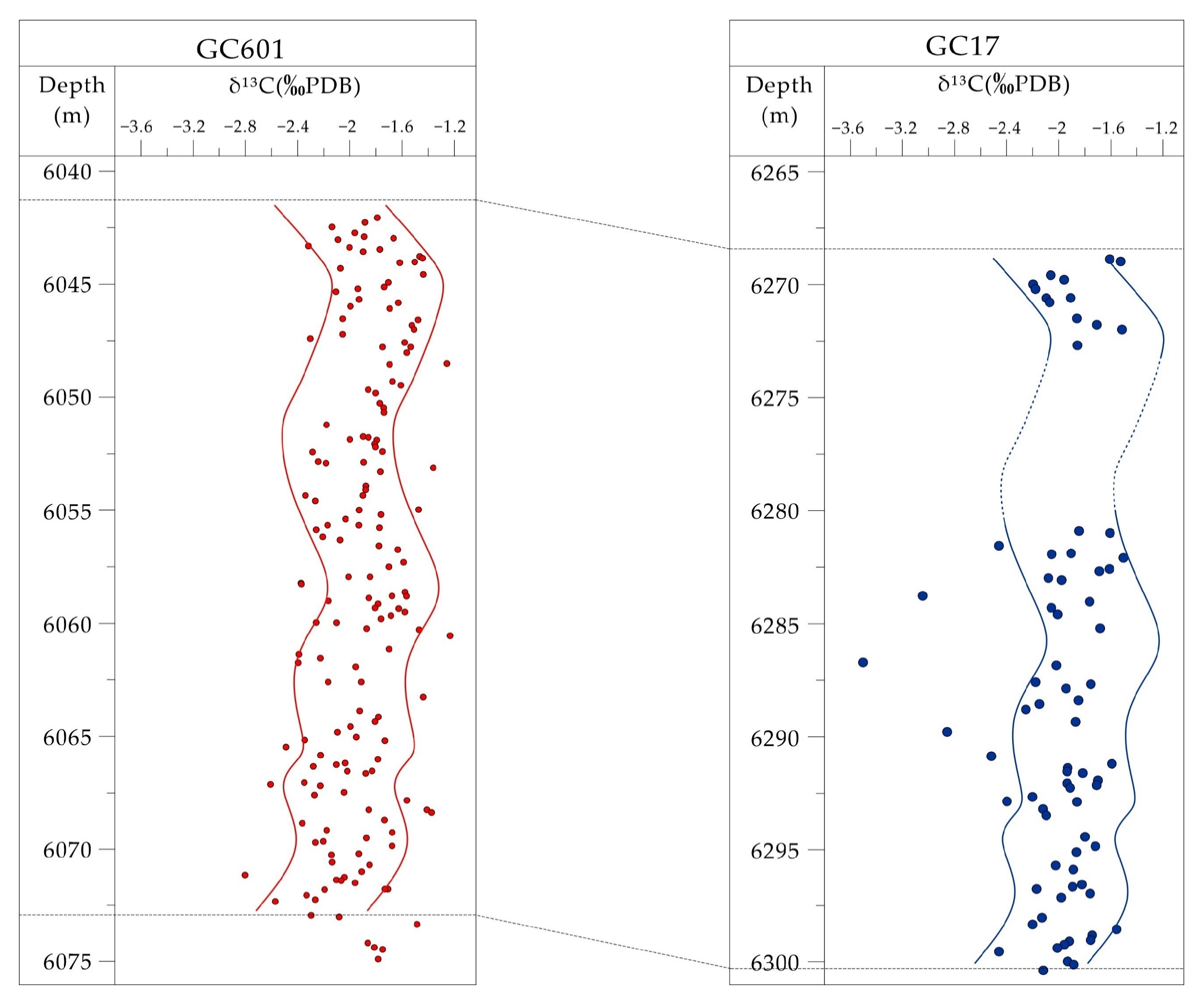
5.1. Correlation by Fischer Plot

In the current work, the Python program coded by Yang [2] was employed for automatic plotting based on GR curves, overcoming the subjectivity caused by manual identification of cycles. The Fischer plots (Figure 6) of the two wells, highly correlated with one another, demonstrate that sea-levels of the middle and upper parts of the Ying 3 member fluctuate and the variation is characterized by falling, then rising, subsequently maintaining, and finally dropping again. This trend is consistent with the second-order sea-level fluctuation of the Tarim Basin [10], and the third-order sea-level change curve of the Ying 3 member in the southeast Tarim [3], which provides good support for the application of such a method. A comparison of the Fischer plots of the middle and upper parts of the Ying 3 Member of these two wells shows that there are locally minor differences in high-frequency cycles, with overall consistency, which may result from multiple interpretations of GR logs or local differences in sedimentary palaeogeomorphology. GR logs work with the key inflection points in the Fischer plots together to fulfill the depth correlation between the two wells—5995 m in Well GC601 corresponds to 6223 m in Well GC17 (Figure 6).

5.2. Reconstruction of Carbon Isotope Comprehensive Curve

Geochemical features of ancient carbonate rocks are prone to changes triggered by later diagenesis, resulting in partial or complete loss of geochemical information of seawater in the original sedimentary period [38,52]. It is necessary to ensure that the carbon and oxygen isotope data are reliable to reflect the characteristics of the original seawater. A commonly used method for reliability evaluation is to check whether the carbon and oxygen isotope values of the samples are correlated [54]. Because of a more sensitivity of the oxygen isotopes, rather than the carbon isotopes, to the diagenetic alteration, higher correlations between carbon and oxygen isotope values indicate that the carbon and oxygen isotopes are subjected to coordinated changes during diagenesis, and the data are far from reliable; on the contrary, when the correlation is low, samples are less affected by the diagenetic alteration, of which isotopic values can reflect the isotope composition of the original seawater [55]. Therefore, when the carbon and oxygen isotope values of Wells GC601 and GC17 were cross plotted, it was found that δ13C and δ18O of the two wells are highly scattered with no distinct linear correlation (Figure 7), and the data are thus considered reliable.
When the δ13C data of Wells GC601 and GC17 were mapped by depth (Figure 5) and displayed with a proper vertical scale and identical horizontal scale range, a fluctuating pattern can then be identified, which is consistent with the periodic rise and fall of sea-levels. Due to the periodic and random fluctuations, the original δ13C data fluctuated fiercely; it is not easy to make a direct comparison or to identify high-frequency cycles. However, by comparing the envelopes of the data points, it can still be found that the δ13C fluctuation at 6267–6300 m of Well GC17 and 6043–6076 m of Well GC601 are in line with each other (Figure 8), and the corresponding depth correlation complies with that drawn from the Fischer plots (Figure 6), indicating that this correlation makes the carbon isotope curve mergence feasible. After the implementation of the 5-point moving average smoothing, the data points become more convergent, and the fluctuation trend becomes more obvious (Figure 9, smoothed δ13C column). The smoothed δ13C data can be merged by the depth correlation drawn from the Fischer plots, and then the high-frequency carbon isotope fluctuation curve of the whole middle and upper parts of the Ying 3 member in the Gucheng area can be obtained (Figure 9).

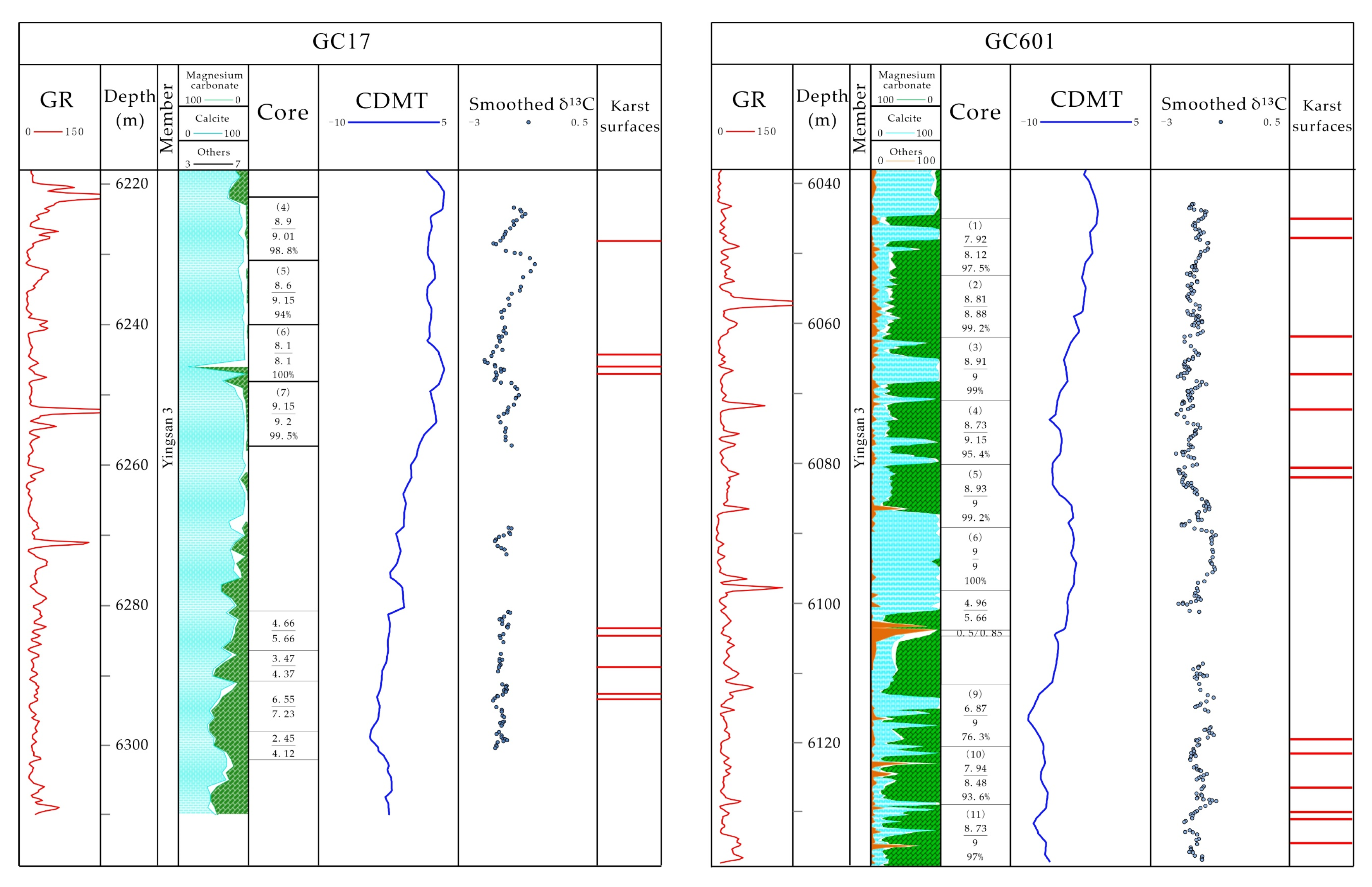
5.3. Verification of Carbon Isotope Comprehensive Curve

In this study, bulk rock REE analysis was carried out in 52 core samples from Wells GC17 and GC601, with δCe calculated. The REE analysis and δCe calculation results were then mapped by depth, revealing that the interval with a positive carbon isotope value anomaly is accompanied by the negative deviation of δCe; on the contrary, the positive deviation of δCe tends to occur in the case of negative deviation of the carbon isotope value. In addition, the strontium isotope ratio of the interval with the negative carbon isotope deviation is often higher than that of the Ordovician seawater, implying the influences of the meteoric freshwater. Therefore, it is concluded that the high-frequency carbon isotope value fluctuation can work as the high-frequency sea-level changes, and four fourth-order cycles, and 21 high-frequency cycles were identified by the curve (Figure 10).

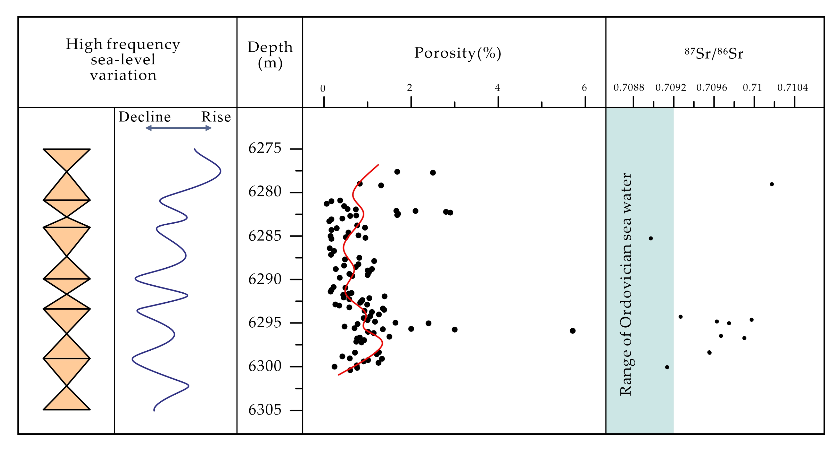
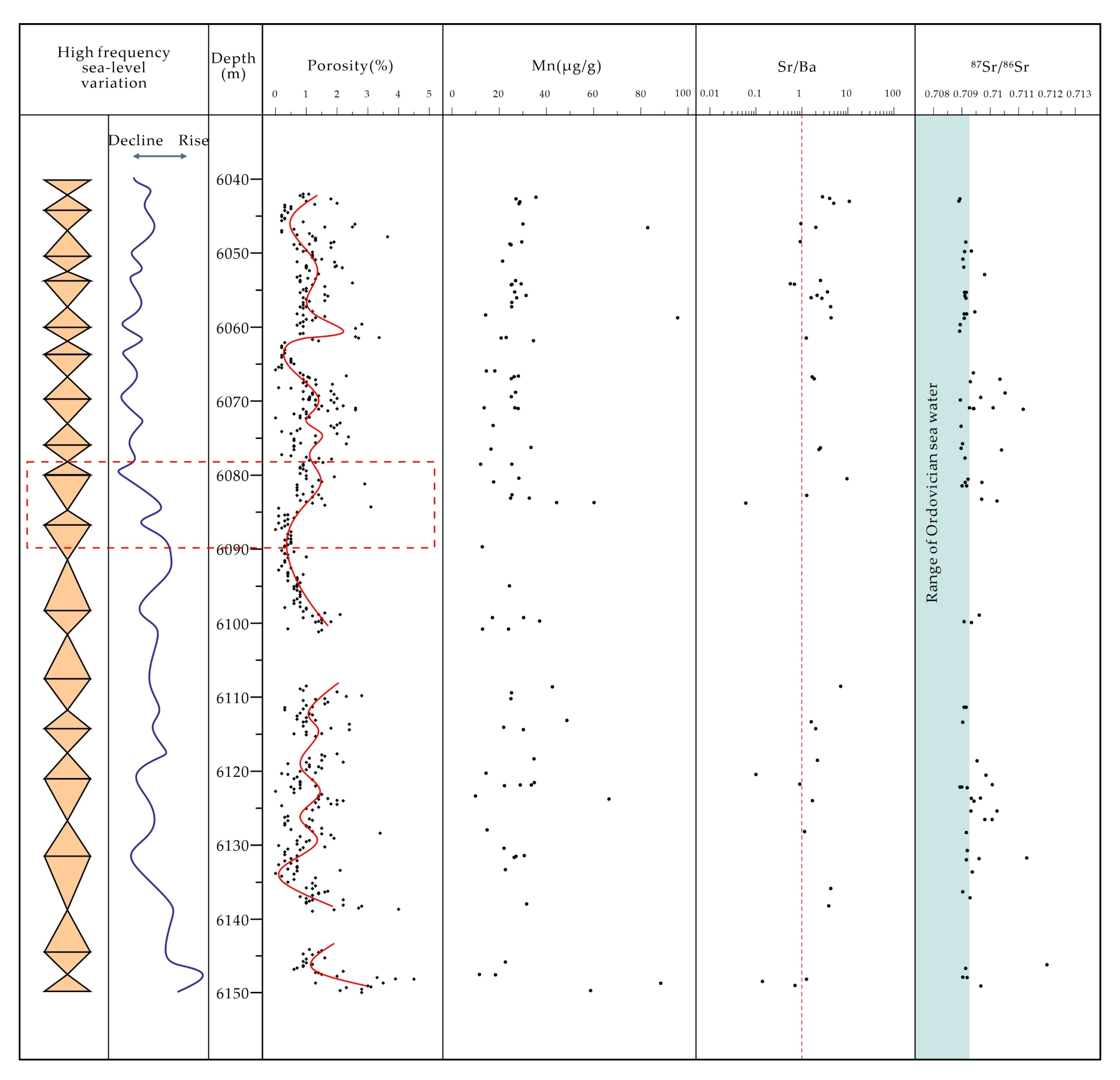
5.4. Relation between High-Frequency Sea-Level Changes and Reservoir Characteristics

The current work carried out some analyses to explore the way high-frequency sea-level changes affect the carbonate ramp shoal facies dolomite reservoir, namely macroscopic core observation, thin section microscopic analysis, reservoir physical property testing, and geochemical testing. More than 20 cyclic karst surfaces as a result of the penecontemporaneous exposure dissolution were identified based on the systematic observation of the dolomite cores of the Ying 3 member in Wells GC17 and GC601 (Figure 11). These karst surfaces are commonly filled with sparry calcuate, due to the irregular space created by karstification, and macroscopically feature chaotic and mottling and a common geopetal texture. The microscopy also reveals typical karst features, such as the geopetal fabric and the vadose zone of silts (Figure 2i,j and Figure 12). Additionally, the δ13C has seen considerable negative deviations near karst surfaces.
The measured porosity of the shoal facies dolomite cores from 6280–6300 m of Well GC17 is mapped by depth (trend is marked in red line) and compared with the high-frequency sea-level change curve of the interval at the same depth of the Ying 3 member issued from the carbon isotope value (Figure 13). In general, there is an obvious negative correlation between both, with dolomite porosity increasing when the high-frequency sea-level falls and decreasing when it rises. Furthermore, at 6295–6300 m, the Sr isotope ratios of the high-porosity samples are much higher than those of the Ordovician seawater (ranging 0.7079–0.7092) [52]. As shown in the high-frequency sea-level change curve, the interval mentioned above responds to one maximum sea regression; however, the distinct positive deviation of the Sr isotope ratio indicates that the exposure dissolution intensifies when the sea-level falls, and thus, a mixture with the terrigenous Sr occurs due to the meteoric freshwater invasion contributing to the development of pores in this interval.
Similarly, when it comes to mapping the porosity of the continuously-cored shoal facies dolomite ranging from 6040–6150 m (nearly 90 m, trend is marked in red line) of Well GC601 by depth (Figure 14), we find that the correlation between the porosity and the high-frequency sea-level change is negative as well, even over an extensive interval, which is consistent with the pattern in Well GC17. In addition, the Sr isotope ratio is often higher in the intervals with high porosity than that of the seawater of the same period. The REE pattern of samples from the karst surface showed a negative anomaly of element Eu (Figure 15), which means they experienced modification by low temperature and oxidizing fluid in the penecontemporaneous period. This is also evidence of exposure.
Core analysis of Well GC601 shows that such penecontemporaneous exposure dis-solution occurs frequently during the sea-level falling, with the corresponding cycle thick-ness even at the meter scale. For example, the interval ranging from 6080–6089 m responds to an obvious high-frequency sea-level fall (Figure 14, marked by dashed box). When the vertical scale is enlarged (Figure 16), we can recognize several obvious meter-scale cycles in the carbon isotope value variation, which is highly consistent with the core records, showing that the high-frequency sea-level falling is associated with the frequent exposure and modification of the shallow-water ramp belt. Furthermore, pore-vug intervals are primarily found near the karst exposure surface. Such intervals, recognized either by cores or thin sections, are generally located under the karst exposure surface (Figure 13). The tight dolomite with less porosity of the grain shoal facies occurs in an alternating manner with the porous dolomite of the grain shoal facies, resulting in many upward-shallowing cycles. Pores tend to develop closer to the top cycle, which demonstrates that the physical properties of the dolomitized reservoirs of the shoal facies are dependent on the periodic penecontemporaneous exposure dissolution.

5.5. Limitations and Future Work

In the current work, a relatively reliable high-frequency sea-level change curve of the Ying 3 member has been built. With the help of this curve, the relation between the shoal facies dolomite reservoir and the high-frequency sea-level cycle was established and examined in Wells GC17 and GC601. Moreover, this study proves that the Fischer plot can be applied in bridging data from different wells. However, there are still several limitations that need to be overcome in future work. For example, in the current work, the GR curve was used to build the Fischer plot, which is the key step to correlate these two wells. However, when it comes to some other wells in this area, they may show a less comparable result. This may have resulted in the loss of original sea water environment information during the burial process and diagenesis. To solve this problem, it is necessary to further optimize the logging curve and to do more work on sample selection. If this can be overcome in future work, more data can be applied in the study to build a more accurate sea-level curve. With more wells involved, it may be possible to build a general model of the shoal facies dolomite reservoir.

6. Conclusions

With the Fischer plots used as the basis for the inter-well merging, the carbon isotope data of Wells GC17 and GC601 with high sampling density (the sampling interval is about 0.272 m) were integrated to develop a relatively reliable high-frequency sea-level change curve for the Gucheng area of the Tarim Basin, where four fourth-order cycles and 21 high-frequency cycles have been identified. Moreover, the merged curve shows that the vertical distribution of the porosity of the carbonate ramp shoal dolomite reservoir is closely related to the high-frequency sea-level change. Specifically, the porosity of the dolomite increases with the high-frequency sea-level falling and decreases when it rises. Meanwhile, the karst exposure surface is developed at the top of the upward-shallowing cycle due to the frequent exposure and modification of the shallow-water ramp belt when the high-frequency sea-level falls. The pore-vug reservoirs are concentrated below the karst exposure surface, and pores are more developed closer to the top of the cycle, indicating that the properties of the dolomitized reservoirs of the shoal facies are dominated by the penecontemporaneous periodic exposure dissolution.

Author Contributions

Conceptualization, T.L. and K.Z.; methodology, K.Z. and T.L.; software, Y.Z.; validation, Y.Z., K.Z. and X.Z.; formal analysis, K.Z. and T.L.; investigation, T.L.; resources, T.L. and Y.Z.; data curation, K.Z.; writing—original draft preparation, T.L. and K.Z.; writing—review and editing, Y.Z., X.Z., Q.Y. and B.L.; visualization, K.Z., T.L. and B.L.; supervision, Z.F. and Y.Z.; project administration, Y.Z.; funding acquisition, Y.Z. All authors have read and agreed to the published version of the manuscript.

Funding

This work is supported by the Scientific Research and Technology Development Project of CNPC (grant number 2021DJ0501).

Institutional Review Board Statement

Not applicable.

Informed Consent Statement

Not applicable.

Data Availability Statement

Not applicable.

Acknowledgments

The authors are grateful to the reviewers, whose comments greatly improved the original manuscript.

Conflicts of Interest

The authors declare no conflict of interest.

References

  1. Xiao, J.; Wang, L.; Chen, M.; Chen, Z.; Zhou, J.; Chen, P. Multiple scale fluctuations of the Early Triassic sea level and its influence on reservoirs in the Sichuan Basin. Pet. Geol. Exp. 2017, 39, 618–624. [Google Scholar]
  2. Yang, D.; Huang, Y.; Chen, Z.; Huang, Q.; Ren, Y.; Wang, C. A Python Code for Automatic Construction of Fischer Plots Using Proxy Data. Sci. Rep. 2021, 11, 10518. [Google Scholar] [CrossRef] [PubMed]
  3. He, F.; Lin, C.; Liu, J.; Zhang, Z.; Zhang, J.; Yan, B.; Qu, T. Migration of the Cambrian and Middle-Lower Ordovician carbonate platform margin and its relation to relative sea level changes in southeastern Tarim Basin. Oil Gas Geol. 2017, 38, 711–721. [Google Scholar]
  4. Read, J.F. Carbonate Platforms of Passive (Extensional) Continental Margins: Types, Characteristics and Evolution. Tectonophysics 1982, 81, 195–212. [Google Scholar] [CrossRef]
  5. Mei, M. From vertical stacking pattern of cycles to discerning and division of sequences: The third advance in sequence stratigraphy. J. Palaeogeogr. 2011, 13, 37–54. [Google Scholar]
  6. Wang, Q.; Han, J.; Li, H.; Sun, Y.; He, H.; Ren, S. Carbonate sequence architecture, sedimentary evolution and sea level fluctuation of the Middle and Lower Ordovician on outcrops at the northwestern margin of Tarim Basin. Oil Gas Geol. 2019, 40, 835–850, 916. [Google Scholar]
  7. Zhang, Y.; Chen, J.; Zhou, J.; Yuan, Y. Sedimentological Sequence and Depositional Evolutionary Model of Lower Triassic Carbonate Rocks in the South Yellow Sea Basin. China Geol. 2019, 2, 301–314. [Google Scholar] [CrossRef]
  8. Jamaludin, S.N.F.; Pubellier, M.; Menier, D. Structural Restoration of Carbonate Platform in the Southern Part of Central Luconia, Malaysia. J. Earth Sci. 2018, 29, 155–168. [Google Scholar] [CrossRef]
  9. Li, W.; Zhang, J.; Hao, Y.; Ni, C.; Tian, H.; Zeng, Y.; Yao, Q.; Shan, S.; Cao, J.; Zou, Q. Characteristics of carbon and oxygen isotopic, paleoceanographic environment and their relationship with reservoirs of the Xixiangchi Formation, southeastern Sichuan Basin. Acta Geol. Sin. 2019, 93, 487–500. [Google Scholar]
  10. Bao, Z.; Jin, Z.; Sun, L.; Wang, Z.; Wang, Q.; Zhang, Q.; Shi, X.; Li, W.; Wu, M.; Gu, Q.; et al. Sea-Level Fluctuation of the Tarim Area in the Early Paleozoic: Respondence from Geochemistry and Karst. Acta Geol. Sin. 2006, 80, 366–373. [Google Scholar]
  11. Gao, D.; Lin, C.; Hu, M.; Huang, L. Using Spectral Gamma Ray Log to Recognize High-frequency Sequences in Carbonate Strata: A case study from the Lianglitage Formation from Well T1 in Tazhong area, Tarim Basin. Acta Sedimentol. Sin. 2016, 34, 707–715. [Google Scholar]
  12. Zong, Y.; Shen, Y.; Qin, Y.; Jin, J.; Liu, J.; Tong, G.; Zheng, J.; Zhang, Y. High Frequency Cyclic Sequence Based on the Milankovitch Cycles in Upper Permian Coal Measures in Panxian, Western Guizhou Province. Geol. J. China Univ. 2019, 25, 598–609. [Google Scholar]
  13. Wang, G.; Deng, Q.; Tang, W. The application of spectral analysis of logs in depositional cycle studies. Pet. Explor. Dev. 2002, 29, 93–95. [Google Scholar]
  14. Zhang, Z.; Zhang, C.; He, Z. Recognition of Stratigraphic High-frequency Cyclical Properties with Sliding Window Spectrum of Logs. J. Oil Gas Technol. 2003, 25, 56–58. [Google Scholar]
  15. Yi, H. Application of well log cycle analysis in studies of sequence stratigraphy of carbonate rocks. J. Palaeogeogr. 2011, 13, 456–466. [Google Scholar]
  16. Shao, C.; Fan, T.; Sun, Y. A case study on Yaojia formation of Changyuan district: Fischer plot analysis based on natural gamma data. Resour. Ind. 2013, 15, 64–70. [Google Scholar]
  17. Liu, Y.; Meng, X. The sea-level change forcing cycies of oolitic carbonate and cycioc-hrological applications. Chin. J. Geol. 1999, 4, 442–450. [Google Scholar]
  18. Amour, F.; Mutti, M.; Christ, N.; Immenhauser, A.; Benson, G.S.; Agar, S.M.; Tomás, S.; Kabiri, L. Outcrop Analog for an Oolitic Carbonate Ramp Reservoir: A Scale-Dependent Geologic Modeling Approach Based on Stratigraphic Hierarchy. AAPG Bull. 2013, 97, 845–871. [Google Scholar] [CrossRef]
  19. Ma, X.; Yang, Y.; Wen, L.; Luo, B. Distribution and exploration direction of medium- and large-sized marine carbonate gas fields in Sichuan Basin, SW China. Pet. Explor. Dev. 2019, 46, 1–13. [Google Scholar] [CrossRef]
  20. Chen, Y.; Zhang, J.; Li, W.; Pan, L.; She, M. Lithofacies paleogeography, reservoir origin and distribution of the Cambrian Longwangmiao Formation in Sichuan Basin. Mar. Orig. Pet. Geol. 2020, 25, 171–180. [Google Scholar]
  21. Wang, Z.; Yang, H.; Qi, Y.; Chen, Y.; Xu, Y. Ordovician gas exploration breakthrough in the Gucheng lower uplift of the Tarim Basin and its enlightenment. Nat. Gas Ind. 2014, 34, 1–9. [Google Scholar]
  22. Zhang, Y.; Li, Q.; Zheng, X.; Li, Y.; Shen, A.; Zhu, M.; Xiong, R.; Zhu, K.; Wang, X.; Qi, J.; et al. Types, evolution and favorable reservoir facies belts in the Cambrian-Ordovician platform in Gucheng-Xiaotang area, eastern Tarim Basin. Acta Pet. Sin. 2021, 42, 447–465. [Google Scholar]
  23. Liu, Y.; Hou, J.; Li, Y.; Dong, Y.; Ma, X.; Wang, X. Characterization of Architectural Elements of Ordovician Fractured-cavernous Carbonate Reservoirs, Tahe Oilfield, China. J. Geol. Soc. India 2018, 91, 315–322. [Google Scholar] [CrossRef]
  24. Chen, H.; Zhong, Y.; Hou, M.; Lin, L.; Dong, G.; Liu, J. Sequence Styles and Hydrocarbon Accumulation Effects of Carbonate Rock Platform in the Changxing-Feixianguan Formations in the Northeastern Sichuan Basin. Oil Gas Geol. 2009, 30, 539–547. [Google Scholar]
  25. Zhu, Y.; Ni, X.; Liu, L.; Qiao, Z.; Chen, Y.; Zheng, J. Depositional Differentiation and Reservoir Potential and Distribution of Ramp Systems during Post-rift Period: An example from the Lower Cambrian Xiaoerbulake Formation in the Tarim Basin, NW China. Acta Sedimentol. Sin. 2019, 37, 1044–1057. [Google Scholar]
  26. Huang, X.; Fu, M.; Zhao, L.; Zhou, W.; Wang, Y. Identification and sgnificance of meter-scale cycle of carbonate rocks in Mishrif Formation, HF Oilfield, Irag. Mar. Orig. Pet. Geol. 2019, 24, 44–50. [Google Scholar]
  27. Handford, C.R.; Loucks, R.G. Carbonate Depositional Sequences and Systems Tracts–Responses of Carbonate Platforms to Relative Sea-Level Changes: Chapter 1. 1993. Available online: http://archives.datapages.com/data/specpubs/seismic2/data/a168/a168/0001/0000/0003.htm (accessed on 9 May 2021).
  28. Feng, J.; Zhang, Y.; Zhang, Z.; Fu, X.; Wang, H.; Wang, Y.; Liu, Y.; Zhang, J.; Li, Q.; Feng, Z. Characteristics and main control factors of Ordovician shoal dolomite gas reservoir in Gucheng area, Tarim Basin, NW China. Pet. Explor. Dev. 2022, 49, 45–55. [Google Scholar] [CrossRef]
  29. Zhang, J.; Hu, M.; Feng, Z.; Li, Q.; He, X.; Zhang, B.; Yan, B.; Wei, G.; Zhu, G.; Zhang, Y. Types of the Cambrian platform margin mound-shoal complexes and their relationship with paleogeomorphology in Gucheng area, Tarim Basin, NW. Pet. Explor. Dev. 2021, 48, 94–105. [Google Scholar] [CrossRef]
  30. Cao, Y.; Wang, S.; Zhang, Y.; Yang, M.; Yan, L.; Zhao, Y.; Zhang, J.; Wang, X.; Zhou, X.; Wang, H. Petroleum geological conditions and exploration potential of Lower Paleozoic carbonate rocks in Gucheng Area, Tarim Basin, China. Pet. Explor. Dev. 2019, 46, 1099–1114. [Google Scholar] [CrossRef]
  31. Zhang, J.; Feng, Z.; Li, Q.; Zhang, B. Evolution of Cambrian mound-beach gas reservoirs in Gucheng platform margin zone, Tarim Basin. Pet. Geol. Exp. 2018, 40, 655–661. [Google Scholar]
  32. Shen, A.; Fu, X.; Zhang, Y.; Zheng, X.; Liu, W.; Shao, G.; Cao, Y. A study of source rocks & carbonate reservoirs and its implication on exploration plays from Sinian to Lower Paleozoic in the east of Tarim Basin, northwest China. Nat. Gas Geosci. 2018, 29, 1–16. [Google Scholar]
  33. Ren, Y.; Zhang, J.; Qi, J.; Zhang, Y.; Zhang, B.; Liu, Y. Sedimentary characteristics and evolution laws of Cambrian-Ordovician carbonate rocks in tadong region. Pet. Geol. Oilfield Dev. Daqing 2014, 33, 103–110. [Google Scholar]
  34. Zhang, Y.; Gao, Z.; Li, J.; Zhang, B.; Gu, Q.; Lu, Y. Identification and distribution of marine hydrocarbon source rocks in the Ordovician and Cambrian of the Tarim Basin. Pet. Explor. Dev. 2012, 39, 285–294. [Google Scholar] [CrossRef]
  35. Jiang, M.; Zhu, J. Carbon and strontium isotopic characteristics of Ordovician carbonate rocks in the Tarim Basin and their responses to sea level changes. Sci. Sin. 2002, 32, 36–42. [Google Scholar]
  36. Zhao, G. Middle-Late Ordovician Sea-Level Changes in the Bachu Area, Tarim Basin, Xinjiang: Carbon, Oxygen and Strontium Isotope Records. Ph.D. Thesis, Jilin University, Changchun, China, 2013. [Google Scholar]
  37. Kaufman, A.J.; Knoll, A.H. Neoproterozoic Variations in the C-Isotopic Composition of Seawater: Stratigraphic and Biogeochemical Implications. Precambrian Res. 1995, 73, 27–49. [Google Scholar] [CrossRef]
  38. Hoefs, J. Stable Isotope Geochemistry, 6th ed.; Springer: Berlin, Germany, 2009. [Google Scholar]
  39. Liu, C.; Zhang, Y.; Li, H.; Cao, Y.; Zhao, Y.; Yang, M.; Zhou, B. Sequence stratigraphy classification and its geologic implications of Ordovician Yingshan formation in Gucheng area, Tarim basin. J. Northeast. Pet. Univ. 2017, 41, 82–96. [Google Scholar]
  40. Wenzel, B.; Joachimski, M.M. Carbon and Oxygen Isotopic Composition of Silurian Brachiopods (Gotland/Sweden): Palaeoceanographic Implications. Palaeogeogr. Palaeoclimatol. Palaeoecol. 1996, 122, 143–166. [Google Scholar] [CrossRef]
  41. Cramer, B.D.; Saltzman, M.R. Sequestration of 12C in the Deep Ocean during the Early Wenlock (Silurian) Positive Carbon Isotope Excursion. Palaeogeogr. Palaeoclimatol. Palaeoecol. 2005, 219, 333–349. [Google Scholar] [CrossRef]
  42. Fischer, A.G. The Lofer Cyclothem of the Alpine Triassic. In Symposium on cyclic sedimentation. Kans. State Geol. Surv. Bull. 1964, 169, 107–149. [Google Scholar]
  43. Read, J.F.; Goldhammer, R.K. Use of Fischer Plots to Define Third-Order Sea-Level Curves in Ordovician Peritidal Cyclic Carbonates, Appalachians. Geology 1988, 16, 895–899. [Google Scholar] [CrossRef]
  44. Sadler, P.M.; Osleger, D.A.; Montanez, I.P. On the Labeling, Length, and Objective Basis of Fischer Plots. J. Sediment. Res. 1993, 63, 360–368. [Google Scholar]
  45. Day, P.I. The Fischer Diagram in the Depth Domain: A Tool for Sequence Stratigraphy. J. Sediment. Res. 1997, 67, 982–984. [Google Scholar] [CrossRef]
  46. Guo, Y.; Wang, F.; Gan, F.; Yan, B. Forecasting of Spring Flow based on Moving Average Model and Exponential Smoothing Model. J. Hebei GEO Univ. 2020, 43, 19–25. [Google Scholar]
  47. Elderfield, H.; Greaves, M.J. The Rare Earth Elements in Seawater. Nature 1982, 296, 214–219. [Google Scholar] [CrossRef]
  48. Gromet, L.P.; Haskin, L.A.; Korotev, R.L.; Dymek, R.F. The “North American Shale Composite”: Its Compilation, Major and Trace Element Characteristics. Geochim. Cosmochim. Acta 1984, 48, 2469–2482. [Google Scholar] [CrossRef]
  49. Wilde, P.; Quinby-Hunt, M.S.; Erdtmann, B.D. The Whole-Rock Cerium Anomaly: A Potential Indicator of Eustatic Sea-Level Changes in Shales of the Anoxic Facies. Sediment. Geol. 1996, 101, 43–53. [Google Scholar] [CrossRef]
  50. Li, G. The Carbon Isotope Fluctuations and Its Paleoenvironmental Significance of the Upper Jurassic Bulk Carbonate from Amdo Area, Tibet. Ph.D. Thesis, Chengdu University of Technology, Chengdu, China, 2020. [Google Scholar]
  51. Yang, J.; Sun, W.; Wang, Z. Variations in Sr and C Isotopes and Ce Anomalies in Successions from China: Evidence for the Oxygenation of Neoproterozoic Seawater? Precambrian Res. 1999, 93, 215–233. [Google Scholar]
  52. Veizer, J.; Ala, D.; Azmy, K.; Bruckschen, P.; Buhl, D.; Bruhn, F.; Carden, G.A.; Diener, A.; Ebneth, S.; Godderis, Y. 87Sr/86Sr, Δ13C and Δ18O Evolution of Phanerozoic Seawater. Chem. Geol. 1999, 161, 59–88. [Google Scholar] [CrossRef]
  53. Haq, B.U.; Schutter, S.R. A Chronology of Paleozoic Sea-Level Changes. Science 2008, 322, 64–68. [Google Scholar] [CrossRef]
  54. Horacek, M.; Brandner, R.; Abart, R. Carbon Isotope Record of the P/T Boundary and the Lower Triassic in the Southern Alps: Evidence for Rapid Changes in Storage of Organic Carbon. Palaeogeogr. Palaeoclimatol. Palaeoecol. 2007, 252, 347–354. [Google Scholar] [CrossRef]
  55. Mazzullo, S.J.; Harris, P.M. An Overview of Dissolution Porosity Development in the Deep-Burial Environment, with Examples from Carbonate Reservoirs in the Permian Basin. West Tex. Geol. Soc. Midl. TX 1991, 89–91. [Google Scholar]
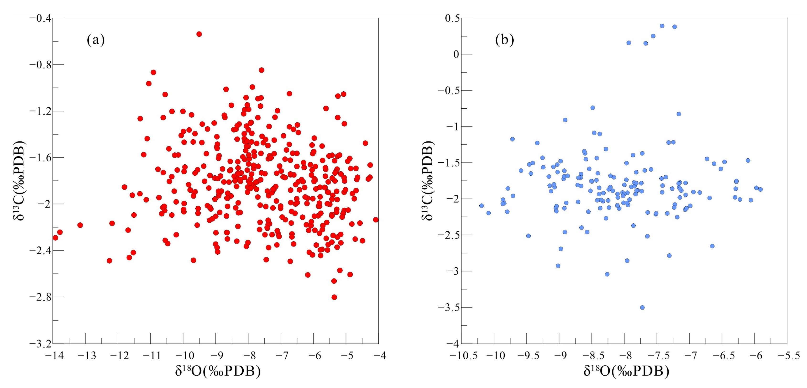
Figure 1. (a) Ordovician lithofacies paleogeography of Tarim basin and location of the Gucheng area; (b) Strata column of the Gucheng area.
Energies 15 04287 g001
Figure 2. Macroscopic and microscopic scale images of typical facies and sedimentary phenomenon in the Ying 3 member. (a) Calcarenite, core sample, GC601 6065.25 m, sand shoals; (b) Calcarenite, plane-polarized light, GC601 6044 m, sand shoals; (c) Dolomite, core sample, cross bedding, GC601 6046.5 m, dolomitized shoals; (d) Dolomite, plane-polarized light, GC601 6061.87 m, dolomitized shoals; (e) Micrite, core sample, pelitic strip, GC601 6162.42 m, inter-shoal marine; (f) Micrite, plane-polarized light, pelitic strip and dolomite crystal, GC601 6047 m, inter-shoal marine; (g) Crystal powder dolomite, core sample, GC601 6067.05 m, tidal flat; (h) Crystal powder dolomite, plane-polarized light, GC601 6067.05 m, tidal flat; (i) Dolomite with karstic mosaic, core sample, GC601 6131.52 m; (j) Crystal dolomite with seepage silt, plane-polarized light, GC601 6066.64 m; (k) Dolomite, plane-polarized light, GC601 6111.36 m, dolomitized shoals; (l) CL image in the same field of vision with (k).
Energies 15 04287 g002
Figure 3. (a) Original concept of Fischer plots introduced by Fischer (1964); (b) Schematic form of Fischer plot in time domain; (c) Schematic form of Fischer plots in depth domain. Cited from Yang et al., 2021 [2].
Energies 15 04287 g003
Figure 4. Steps and workflow of this study.
Energies 15 04287 g004
Figure 5. Original testing data of samples from well GC601 and GC 17.
Energies 15 04287 g005
Figure 6. Fischer plots of well GC601 and GC 17 and their comparison with the previous third-order sea-levels. The global sequence is cited from Reference [53], the sea-level fluctuation of the Tarim Basin is cited from References [3,10].
Energies 15 04287 g006
Figure 7. Cross plot of carbon and oxygen isotope values. (a) GC601. (b) GC17.
Energies 15 04287 g007
Figure 8. Comparison of carbon isotope variation with depth between the two wells.
Energies 15 04287 g008
Figure 9. The developed comprehensive curve of carbon isotope variation with depth.
Energies 15 04287 g009
Figure 10. Verification of the effectiveness of the merged carbon isotope variation curve with depths to represent sea-level changes. Red arrows showed the trend of δ13C and δCe.
Energies 15 04287 g010
Figure 11. Cyclic karst exposure surfaces in Wells GC17 and GC601.
Energies 15 04287 g011
Figure 12. Macroscopic characteristics of the karst exposure surfaces in Well GC601. Karst surfaces are marked in dashed lines. (a) 6167.52 m. (b) 6125.37 m. (c) 6109.81 m. (d) 6067.15 m. (e) 6167.7 m. (f) 6122.12 m. (g) 6079.12 m. (h) 6057.84 m.
Energies 15 04287 g012
Figure 13. Correlation between reservoir porosity and high-frequency sea-levels and Sr isotope ratio characteristics in GC17. The red line showed the trend of porosity.
Energies 15 04287 g013
Figure 14. Correlation between reservoir porosity and high-frequency sea-levels and other geochemical evidence in GC601. The red line showed the trend of porosity. The part in dashed box will be showed in Figure 16.
Energies 15 04287 g014
Figure 15. The REE pattern of samples from the karst surface. Each line with colors represents one sample from karst surface.
Energies 15 04287 g015
Figure 16. Variation pattern of the meter-scale cycles in Well GC601. Red arrows showed the trend of δ13C.
Energies 15 04287 g016
Table 1. An overview of experimental data statistics.
Well No.AnalysisAmountResult Range
GC 601C-O isotope396δ13C: −2.802%~−0.537%
δ18O: −13.917%~−4.085%
87Sr/86Sr730.708896~0.712001
δCe40−0.0746~0.0287
GC 17C-O isotope151δ13C: −2.927%~−0.740%
δ18O: −10.190%~−5.909%
87Sr/86Sr120.708927~0.710174
δCe12−0.0456~−0.0031
Publisher’s Note: MDPI stays neutral with regard to jurisdictional claims in published maps and institutional affiliations.

