Analysis of Business Customers’ Energy Consumption Data Registered by Trading Companies in Poland

Abstract

In this article, we analyze the energy consumption data of business customers registered by trading companies in Poland. We focus on estimating missing data in hourly series, as forecasts of this frequency are needed to determine the volume of electricity orders on the power exchange or the contract market. Our goal is to identify an appropriate method of imputation missing data for this type of data. Trading companies expect a specific solution, so we use a procedure that allows to choose the imputation method, which will consequently improve the accuracy of forecasting energy consumption. Using this procedure, a statistical analysis of the occurrence of missing values is performed. Then, three techniques for generating missing data are selected (missing data are generated in randomly selected series without missing values). The selected imputation methods are tested and the best method is chosen based on MAE and MAPE errors.

1. Introduction

Time series analysis is widely used in many management systems, in the areas of: transport systems, including urban transport [1,2,3,4] environment [5,6,7,8], medical data [9,10,11,12,13,14,15] and energy [16,17,18,19,20,21]. In this work, we analyze data on electricity consumption. As emphasized by Wang et al. [21], economic development causes an increase in electricity demand, and thus generates the need to save energy, i.e., better and better energy management systems. Such systems are mainly dedicated to electricity consumers, but effective energy management is also crucial for electricity trading companies. In their activities, in addition to commercial problems and challenges, such companies must often purchase energy on the wholesale market and then distribute it to individual customers. There is a need to ensure continuous and accurate balancing of electricity demand and production in this process. This is due to, among other things, the inability to store the purchased product, as well as the need to balance the demand for electricity with the supply at any time. Therefore, it is very valuable to know about electricity demand in the near and far horizon, i.e., energy consumption schedules. Such schedules can be defined as a set of data specifying the amount of electricity planned to be introduced or taken from the grid for particular periods (e.g., day, week, month or year). Standardization of such a schedule leads to developing a profile characteristic for a given recipient or group of recipients. Therefore, it is important in this context to increase the accuracy of forecasting electricity consumption, which depends on the quality of the collected data [7,22].

The specificity of electricity trading requires the analysis of hourly data, because forecasts of such frequency are needed to determine the volume of electricity orders on the power exchange or contract market, and then, if necessary, to correct these orders. Despite the intensive development of smart metering and the installation of an increasing number of meters ensuring the possibility of transmitting hourly values, only a dozen or so percent (a small percentage) of concluded contracts are settled based on these measurements. In most cases, electricity distributors only provide the seller with the total amount of energy consumed by the consumer during the load period, which varies from a few days to a year. Periodic readouts are then distributed in the time series with an hourly gradation using standard profiles developed by distributors. Execution of a new contract with the customer requires preparing a consumption forecast for its whole term. To create the forecast, the data of energy consumption by the customer in preceding periods or the declared energy consumption for a new building is required. However, the acquired historical data is not often complete and contains missing values. This is a common problem when data is measured and recorded [23,24]. Various reasons lead to a lack of values in the time series. In the case of energy consumption data, these can be communication errors, sensor failures, or power outages [25], but also missing values due to the lack of readings (values are then not measured).

The extensive literature on the imputation of missing data shows algorithms for replacing missing data with estimates [26]. The most common data imputation techniques rely on correlations between attributes to estimate values for missing data. These include: Multiple Imputation [27], Expectation-Maximization [28], Nearest Neighbor [29], and Hot Deck [30]. Many studies show examples of multidimensional time series imputation [1,4,31,32,33,34,35]. However, in the case of univariate series, there are no additional attributes, therefore imputation algorithms specially adapted to such data should be used [23]. For example, Bokde et al. [25] propose the ‘imputePSF’ method, which is a modification of the pattern sequence based forecasting (PSF) method, while Demirhan and Renwick [5] compare the performance of the methods available in the ‘imputeTS’ package, which are dedicated to univariate time series with irregular intervals.

An important element to pay attention to when using imputation methods is the type of data. Depending on the field from which they originate, the data may be characterized by the presence of a trend, seasonality or randomness, or property known as the effect of volatility clustering (volatility in one subperiod depends on the volatility realized in preceding periods). Since series from different fields have distinct characteristics, different imputation methods give better results for the series.

In our study, we analyze anonymised data from Polish energy trading companies. These companies buy electricity wholesale and then sell it to direct customers. It should be emphasized that the trading company does not have direct access to measuring devices and does not read them. The owner of the metering devices (energy meters) from which the readings of energy consumption come is the distribution network operator (DNO). The DNO is obliged to provide the trading company with data on the consumption of the recipient for whom this company provides services related to the sale of energy. Based on these data, the trading company accounts for energy recipients and balances supply and demand on the energy market. Intensive work is underway in Poland to ensure that most of the data for billing comes from smart meters in the form of hourly readings, but at the moment, it is still a problem.

After analyzing many of the previously cited works on the imputation of missing values, we noticed a certain limitation in the applicability of the widely discussed methods and techniques to the analysis of our data. This limitation is the type of data we received from trading companies, which had the form of one-dimensional series and did not contain additional attributes (we only know energy consumption at a given point of electricity consumption—PPE). Therefore, we decided to develop a procedure adapted to the received data, which would allow us to choose the appropriate method of the imputation of the missing value, which could be used by trading companies.

Our procedure allows you to select the best of the tested imputation methods along with the error evaluation, and requires the use of a series with both missing values and no gaps. First, we perform a statistical analysis of the occurrence of missing values in the series to select the techniques for generating missing data. We then use these techniques to generate missing data in randomly selected series without missing data. The selected methods and variants of imputation are compared based on MAPE (mean absolute percentage error) and MAE (mean absolute error) errors calculated for individual points of electricity consumption (PPE) based on real values and imputed values. A detailed description of the procedure is provided in Section 3.4. The results of our research will allow for more accurate forecasts and thus for better planning of purchases by trading companies. The presented research focuses mainly on business customers due to the frequency of readings from energy meters. For this group of customers, data are provided from smart meters similar to other European countries. The results of our work may therefore also be interesting for other energy trading markets.

2. Data

The quality of electricity consumption data is a critical issue in mining big data relating to the energy industry [22]. Thanks to the analysis of this data, it is possible to extract valuable knowledge to increase the level of profitability of energy companies as well as electricity trading companies. Electricity data quality issues can be divided into three categories: noise data—including logical errors and inconsistent data, incomplete data, and outlier data [22]. The problem faced by trading companies that provided data primarily concerns incomplete data, i.e., data containing missing values. As mentioned earlier, the specificity of the electricity market requires paying particular attention to hourly data and such series are discussed in this article.

Data of business customers in Poland from tariff groups B and C were analyzed in detail, as the recipients of these tariffs account for 79% of all customers of trading companies that agreed to provide data for the research. Tariff B is the Medium Voltage used by large enterprises (excluding the largest recipients such as mines or large factories), while Tariff C is the Low Voltage dedicated to small and medium-sized enterprises (mainly service and trade companies). The data of individual customers were excluded from the study, because for them, energy readings are carried out at large intervals (even every few months) and, as indicated, are not the main customers of the surveyed trading companies.

Finally, a database consisting of 3236 data series (data from 3236 PPE in 2019) was selected for the analysis with the following characteristics:

• the length of a single sequence of missing data (gaps) not longer than 48 h in one sequence,
• no more than 576 h with missing data during the year,
• no more than 20% of profile consumption (these are values estimated based on profiles prepared by trading companies in the event that the energy consumption readings occur in periods longer than every hour, e.g., once a day or once a week).

Missing Values Analysis

In a database of 3236 data series, 210 series (210 PPE) contained the missing values. For these series, a statistical analysis of the occurrence of missing data was performed. The number of missing values, the number of gaps (a gap is defined as one or more data missing in succession), the longest sequence of missing values, the shortest sequence of missing values, and the average length of gaps were analyzed. Details are provided in

Table 1. Basic statistics of missing data.

Statistics	Number of Missing Values	Number of Gaps	The Longest Sequence of Missing Values	The Shortest Sequence of Missing Values	Average Length of Gaps
min.	1.00	1.00	1.00	1.00	1.00
perc05	1.00	1.00	1.00	1.00	1.00
perc10	1.00	1.00	1.00	1.00	1.00
perc25	3.00	1.00	2.00	1.00	1.00
median	9.00	2.00	4.00	1.00	1.00
perc75	24.00	5.00	13.75	2.75	2.75
perc90	41.50	14.00	24.00	24.00	24.00
perc95	58.20	24.55	24.00	24.00	24.00
max.	463.00	456.00	48.00	48.00	48.00
average	18.80	7.62	9.47	6.00	6.00
std. dev.	37.10	32.82	11.22	10.27	10.27
skewness	8.55	12.26	1.61	2.27	2.27

Source: own elaboration.

.

As shown in Table 1, only 5% of PPE has missing values in more than 58 reading positions. For the indicated points, the number of missing values is not uniformly distributed across all PPE. The number of missing observations is characterized by large right- skewed asymmetry and the presence of outliers (relatively large deviation). The distribution of the number of gaps is a consequence of the distribution of the number of missing observations and is also characterized by large right-skewed asymmetry. In at least 50% of PPEs, the number of gaps does not exceed four (see Table 1, the median for ‘longest gap’ is 4). Lengths of data gaps were also analyzed. As can be seen in Table 1, the longest missing substring of data was 48 (according to the criteria for selecting PPE for imputation).

Figure 1 shows the distribution of the number of missing values (without taking into account the most extreme value). The histogram of the distribution of the number of missing values confirms the earlier comments resulting from the statistical analysis of the occurrence of missing data; a large right-skewed asymmetry can be seen.

Then, the distribution of missing data in terms of the moment of their occurrence was examined. It was noticed that:

• most, because there were as many as 19 cases, of the missing data concerned 3:00 a.m. on 27 November 2019—the time change point (it is worth noting that on this day, the day has 25 h). However, in the second point of the time change on 31 March 2019 at 2 o’clock, no data appeared in the 14 PPE. The problems with the missing values at the time of the time change affected 29 different PPEs, but in only four cases, they occurred simultaneously in the same PPE;
• on 26 January 2019 from 1:00 to 24:00, no data appeared in 15 PPEs;
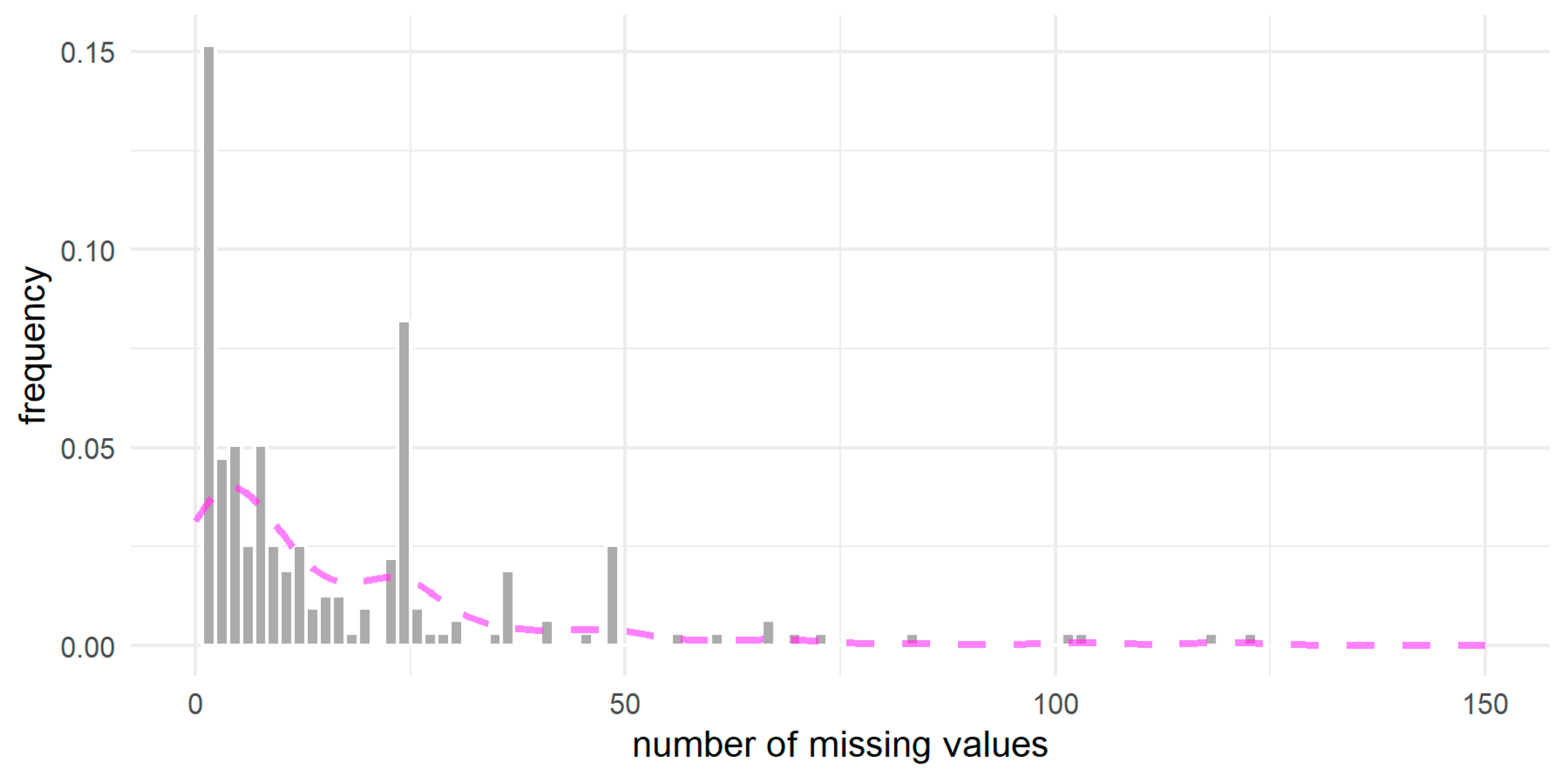
• when examining the distribution of missing values in the indicated set of 210 PPEs, it was found that out of 8760 measurement items—in 6371 (72.7%), there were no missing values in any PPE.

Examples of how missing data can be distributed in the series of consumption are shown in Figure 2, Figure 3 and Figure 4. The figures contain hourly data from three different PPEs with missing values marked (magenta). Collection point PPE-Example1 is an example containing 103 data gaps that occur throughout the analyzed year (see Figure 2). The course of the series for which the number of missing values is 49, and they occur over a period of about one month as shown in Figure 3, while Figure 4 contains the data for the collection point for which there are 48 missing values and they form one gap of 48 h.

When analyzing the processes of the formation of missing data, three mechanisms of their formation can be distinguished [13,24,36]:

• MCAR—missing completely at random—the process of the occurrence of missing data is considered to be completely random (there is no specific mechanism for creating missing values)
• MAR—missing at random—in the process of data occurrence, it is possible to link the occurrence of data with observable variables (there are other variables that affect the existence of missing values, and the probability of their occurrence is independent of the value itself)
• MNAR—missing not at random—in this process, missing data is related to unobservable variables (the probability of a missing value is related to the missing value itself).

It is very important to distinguish between the types of mechanisms that cause missing data because depending on the type of mechanism involved, different methods of imputation missing data will be effective to a different extent. In the case of the data provided, it can be assumed that the mechanism of missing data is of the MCAR or MAR type. Both of these mechanisms allow missing values to be assigned without knowing the specific reasons for their formation.

Taking into account the characteristics of the analyzed series and the adopted mechanism of the occurrence of MCAR or MAR missing data, three techniques for generating artificial missing data were selected:

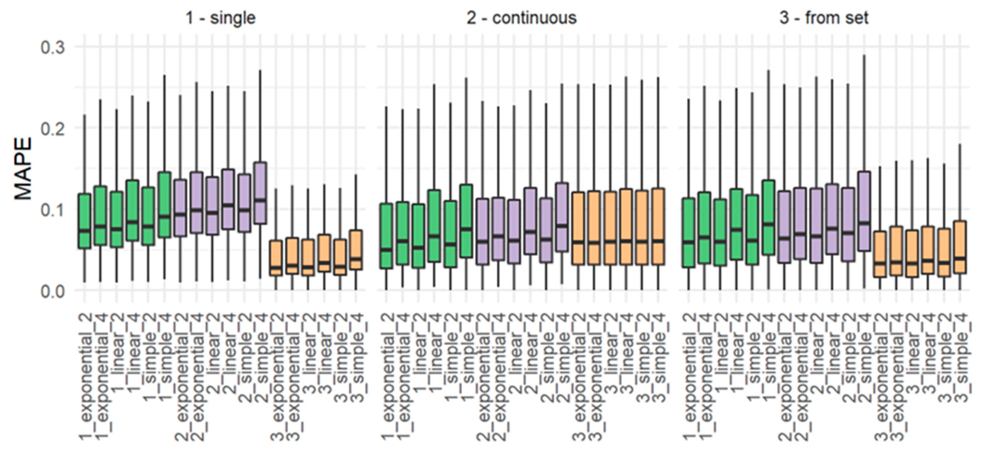
• Random generator—single points—set (1—single). For each of the selected PPEs, 58 locations of missing data were randomly selected. The determined number of missing data was because, for 95% of PPEs with missing data, the number of missing data was not greater than 58 (see Table 1).
• Random generator—continuous data gap—set (2—continuous). For each of the selected PPEs, one gap with a length of 48 was created randomly, i.e., the longest observed missing data (see Table 1).
• Generator based on set 210—set (3—from the set). For each of the selected PPEs with complete data, one PPE was selected at random from a set of 210 imputation candidates. Missing data were inserted in the selected PPE with complete data in the places of their occurrence in the randomly selected PPE from the set of 210.

Missing data generated by the three techniques described above were used in further analyses to test imputation methods.

3. Methods

Many different techniques can be used to deal with missing values [13,37]. These include case deletion, mean substitution, and model-based imputation. According to Strike et al. [38], when a dataset contains less than about 10–15% of missing data, it can simply be removed from the dataset. However, it should be noted that not every dataset is subject to such rules [39], and small amounts of missing data can have a significant impact on the final result of the analysis. This is the problem we deal with in the case of given electricity consumption. As indicated earlier, the quality of such data is of great importance in increasing the accuracy of forecasting, as time series forecasts solely depend on historical data. The proper approach to dealing with missing values in the analyzed case is therefore imputation, which is one of the most reliable ways of dealing with missing values [5].

Depending on the type of data and the field from which the data comes, we have many methods of replacing missing values with estimated values. In the presented research, we have data on energy consumption, provided by energy trading companies, in the form of univariate time series. As emphasized by Moritz et al. [40], univariate time series is a particular challenge in the field of imputation research, and the time series literature focuses almost exclusively on multivariate datasets (as mentioned in the Introduction). Overall, techniques enabling imputation for univariate time series can be divided into three main categories by Moritz et al. [40]:

• One-dimensional algorithms that work with one-dimensional inputs but do not typically use time series characteristics (e.g., mean, mode, median, random sample).
• Univariate time series algorithms that can work with one-dimensional inputs but use time series characteristics. These are algorithms such as last observation carried forward, next observation carried forward, arithmetic smoothing and linear interpolation, and more advanced methods based on structured time series models that deal with seasonality.
• Multivariate algorithms on lagged data, which generally cannot be used for univariate series, but it is possible to add time information as covariates, which allows the use of multivariate imputation algorithms. This can usually be done by using lags (which take the value of another variable from the preceding period) and ‘leads’ (which take the value of another variable in the next period).

In this article, we are looking for solutions that will make the imputation task simple for practitioners (in our case, for trading companies). Therefore, we tested imputation methods that are dedicated to univariate data series, and for testing, we used the R package called ‘imputeTS’ [23].

As mentioned earlier, the subject of the study is the time series of electricity consumption in enterprises. These series are characterized by seasonality, which is related to the cyclical nature of the work of enterprises. The seasonality of the analyzed series was confirmed using the ‘seastests’ package in R. From the set of 3026 series with complete data, 500 series were selected at random. The conducted tests showed that all series were characterized by seasonality.

Analyses based on the characteristics of the tested time series (PPE consumption) prompted us to finally choose three methods of the imputation of missing data: the calendar method, the imputation method by separating the phases of seasonal cycles and the imputation method using seasonality decomposition. Each of the methods was used in three variants related to the seasonality of the time series and the method of taking into account the information used for imputation. Variants of each method relied on the use of a moving average with different ways of incorporating the information ‘closest’ to the time of the missing values.

3.1. Method 1—Calendar Method and 2k Weighted Moving Average Method

The main assumption of this method is taking into account the calendar and dividing the year into subseries. Each subseries refers to a specific time on a specific working day of the week or a specific time of a non-working day (the so-called ‘red’ days). Thus, a single subseries is, e.g., 1 p.m. on working Mondays or 5 p.m. on non-working days.

The moving average algorithm implemented in the ‘imputeTS’ package of the R program was used to impute the missing values. This package is recommended for imputing missing values in time series. The algorithm imputes the missing data with the mean value of the k nearest values ’before’ and ‘after’ the missing values in the series (2k values in total). It was decided that the information necessary for imputation should cover a period of approximately one or two months, therefore $k=2$ or $k=4$ was adopted. The analyses conducted for other values of this parameter confirmed the validity of the findings.

All available methods of weight determination were used in the conducted analyses. The moving average method was with Exponential Weighted Moving Average, Linear Weighted Moving Average and Simple Moving Average.

Exponential weights use the information ageing principle and decrease exponentially with the distance from the missing values—‘observations directly next to the central value $i$, have a weight of $\frac{1}{2}$, the observations one further away (i − 2, i + 2) have a weight of ${\left(\frac{1}{2}\right)}^2$ etc.’. The value of i denotes the number where there is the missing value in the series. Standardized values of exponential weights are determined according to the following Formula (1):

$$w_{j,exponential}=2^{-\left(j+1\right)}{\left({\displaystyle \sum }_{j=1}^k{2}^{-j}\right)}^{-1}$$

(1)

where j is the distance from the missing value (in the immediate vicinity j = 1). For k = 2, $w_{1,exponential}=0.333$, $w_{2,exponential}=0.167$. For k = 4, $w_{1,exponential}=0.267$, $w_{2,exponential}=0.133,w_{3,exponential}=0.067$, $w_{4,exponential}=0.033$.

Linear weighted moving averages also use the information ageing principle, with the denominators of non-standard weights increasing arithmetically—‘the observations directly next to a central value, have weight 1/2, the observations one further away (i − 2, I + 2) have a weight 1/3, etc.’. Therefore, the following weights have the following values: $\frac{1}{2}$,$\frac{1}{3}$,$\frac{1}{4}$… The values of the standardised weights (the number of weights is 2k) can be determined according to the Formula (2):

$$w_{j,linear}={\left[2\left(j+1\right){\displaystyle \sum }_{j=1}^k{\left(j+1\right)}^{-1}\right]}^{-1}$$

(2)

For k = 2, $w_{1,linear}=$ 0.300, $w_{2,linear}=0.200$. For k = 4, $w_{1,linear}=$0.195, $w_{2,linear}=0.130, w_{3,linear}=0.097,w_{4,linear}=0.078$. In the case of a simple moving average, the weights are the same for each value: $w_{j,simple}={\left[2\cdot k\right]}^{-1}.$ For k = 2,$w_{1,simple}=0.250,w_{2,simple}=0.250$.

For correct operation, the algorithm requires at least two real observations to impute a missing value. In the analyzed series, a special series was the series in which the missing value was 7200th hour of the year (25th hour on the day of the time change). In the event of a missing value at that hour, imputation was performed using the moving average algorithm for the entire series. Therefore, in this special situation, the first two values from the hours before the missing value and the first two values after the missing value were taken into account (always k = 2).

3.2. Method 2—Imputation Using Seasonally Splitted Missing Value Imputation

This method relies on imputation by splitting the phases of the seasonal cycles and is implemented in the ‘ImputeTS’ package as the ‘na_seasplit()’ function. Its idea is to split the time series into subseries defined by the phases (seasons) of the seasonal fluctuation cycles, and then impute the values based on the separated seasons. In the conducted analyses, the moving average algorithm was used with the same parameters as in the case of the calendar method. After preliminary analyses, the number of phases was estimated at 168 (1 week = 24 h × 7 days). Therefore, the application of this method consists in distinguishing 168 subseries related to a specific time of the week, and imputation of missing values on the appropriate subseries and the weighted moving average method ($k=2$ or $k=4$). Additionally, in this method, all three available weighting methods were considered.

3.3. Method 3—Imputation Using Seasonally Decomposed Missing Value Imputation

The third method used relied on decomposing the seasonal component from the time series (in the form of a seasonality index), making imputations of missing data on the series without a seasonal component, and then reconsidering the seasonal component. This method is also implemented in the ‘imputeTS’ package as a ‘na_seadec()’ function. Additionally, in this case, the number of phases was considered to be 168 and the weighted moving average algorithm with the values k = 2 or k = 4 was adopted. As shown in the preliminary analyses, a special feature of this method is the ability to generate values outside the acceptable range of variation (negative values). This is due to the correction of the imputed value with the value of the seasonality index. Therefore, in the conducted analyses, a correction to the implemented method was taken into account. The correction consisted in the fact that when the algorithm generated a negative imputed value, this value was changed to zero.

3.4. Comparison of Selected Imputation Methods

The energy consumption data analyzed in this paper contain missing data in actual values. The performance of the imputation methods used was therefore checked for simulated missing data. The procedure for selecting the appropriate missing value imputation method is shown in Figure 5 and can be described step by step as follows:

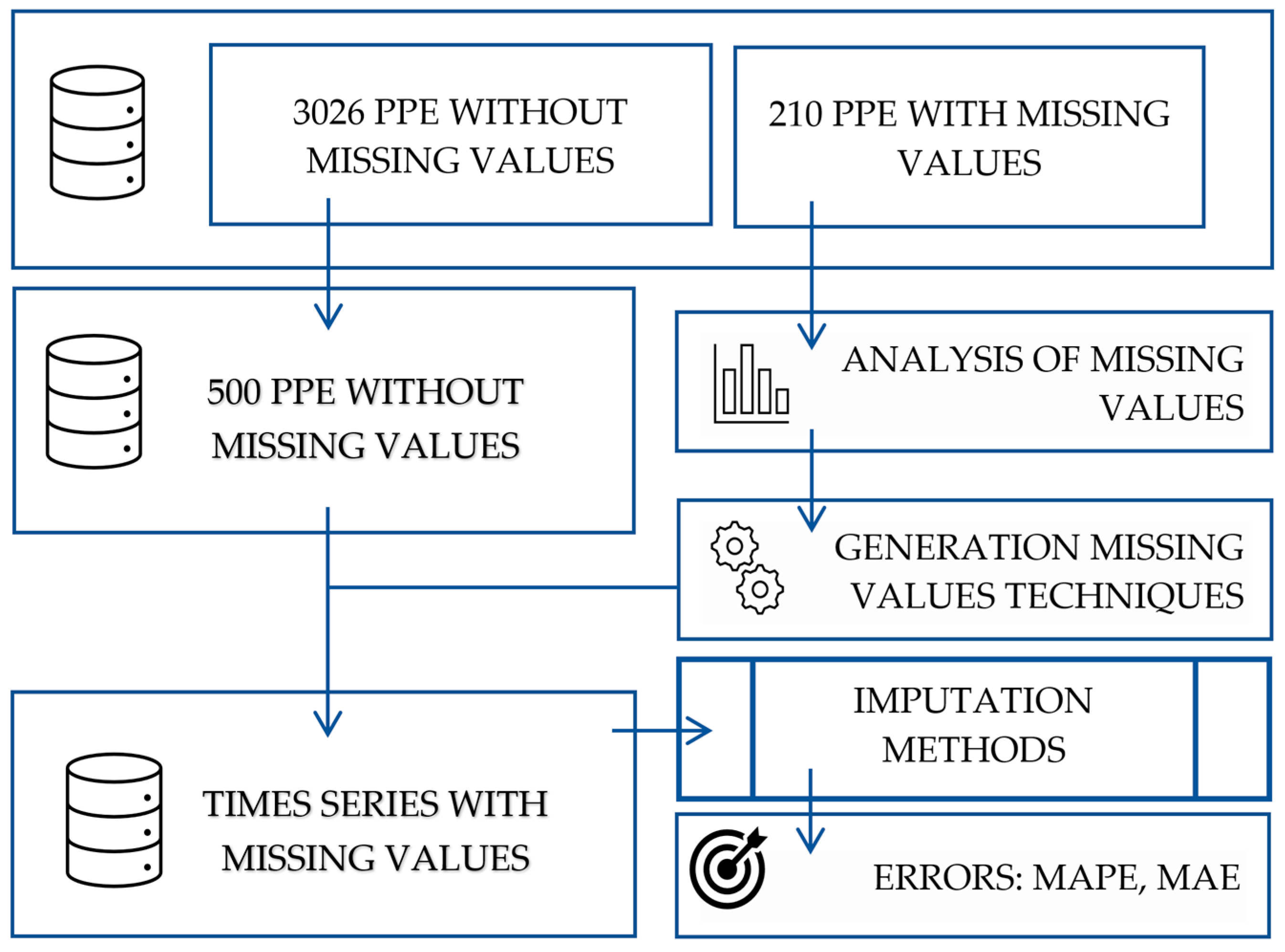
• Step 1. Select from database PPE with missing data.
• Step 2. Perform an analysis of missing data. Determine the number and distribution of missing values.
• Step 3. Prepare techniques for generating missing data adequate to the results of the analysis.
• Step 4. Select a random PPE group from the PPE database without missing data.
• Step 5. Generate missing data according to the generation techniques prepared in step 3.
• Step 6. Apply the selected imputation methods on the series from step 4.
• Step 7. Determine the accuracy of imputation methods based on MAE and MAPE errors.
• Step 8. Select the data imputation method.

To sum up, the acquired database contained 3236 time series. Each of them came from one of several energy suppliers for PPE. In the analyzed database, 210 series contained missing values that had to be imputed. The time series of electricity consumption concerned the B and C business tariffs. We did not have additional information about PPE, such as geographic location or type of business activity. The analysis of the occurrence of missing values in the series allowed for the determination of techniques for generating the missing data. These techniques were used to generate missing values in 500 randomly selected time series. We had information about the actual values in the locations of missing data, and based on this, it was possible to evaluate the indicated imputation methods.

The experiments were carried out for three imputation methods, each method was used in three variants (the moving average method with Exponential Weighted Moving Average, Linear Weighted Moving Average and Simple Moving Average) and each variant was tested for k = 2 for k = 4. This gave us 18 test cases for each technique of generating missing data.

The selected methods and variants of imputation were compared based on the MAPE mean absolute percentage error and the MAE mean absolute error calculated for each PPE based on the actual values and imputed values. These are commonly used metrics to evaluate the performance of imputation methods for time series [21,41,42]. MAE measures the mean size of the errors in the forecast set without taking into account their direction, and MAPE is used to express the mean difference of the absolute errors between the actual and the forecasted values as a percentage of the actual values.

The error $MAPE$ was determined according to the Formula (3):

$$MAPE=\frac{1}{n_{Im{p}_0}}{\displaystyle \sum }_{i\in Im{p}_0}\frac{\left|R_i-I_i\right|}{R_i}$$

(3)

where:

• $Im{p}_0$—a set of indexes of readings for which data has been imputed, with no values for which $R_i=0$,
• $n_{Im{p}_0}$—number of inserted missing values with no values for which $R_i=0$,
• $R_i$—value of actual consumption for the generated missing data,
• $I_i$—imputed consumption value.

The size shows by how much on average the imputed values differed from the actual values for a given PPE, e.g., a value of 0.05 means that the imputed values differed on average by 5%.

The error $MAE$ was determined according to the Formula (4):

$$MAE=\frac{1}{n_{Imp}}{\displaystyle \sum }_{i\in Imp}\left|R_i-I_i\right|$$

(4)

where:

• $Imp$—a set of indexes of readings for which data has been imputed,
• $n_{Imp}$—the number of inserted missing values,
• $R_i$—value of actual consumption for the generated missing data,
• $I_i$—imputed consumption value.

The size informs by how much on average the imputed values differed from the actual values for a given PPE, e.g., a value of 500 means that the imputed values differed on average by 500.

4. Results and Discussion

As mentioned earlier, the variants of the imputation methods were compared based on MAPE (mean absolute percentage error) and MAE (mean absolute error) errors. Error statistics are presented for each variant of the adopted method divided into three imputation methods. Designations of variants of the tested imputation methods were constructed as follows: method_weights_period, e.g., Notation 2_linear_4 means method 2 (imputation with phase/season split) with linear weights and $k=4$ (4 closest values ’before’ and 4 nearest values ’after’ missing)

Figure 6 shows the boxplots of MAPE values for individual methods and their variants broken down into 3 methods of generating missing values. Extremely high values (outliers) were removed from the plot for greater clarity.

Figure 6 shows that in the case of the first set (1—single) and the third set (3—from the set) of generated missing data, imputation method 3 is the most effective. The quartile values for the MAPE error are clearly lower when it is used than for the other methods. Moreover, the best variant of this method is the exponential weights and k = 2. For the second set with missing data, the results are not so unambiguous (method 3 retains the greatest stability for its various variants, but method 1 with the value of k = 2 gives a lower error value).

Figure 7 shows the average values and the 95th percentile values of the MAPE error for individual variants. Similar to earlier, in the case of the first and third method of generating missing values, we can see greater efficiency of the imputation method 3. For the second method of generating missing values (middle panel), there is a clear advantage of imputation method 3 in terms of the average error value.

Figure 8 and Figure 9 present the distributions of MAPE and MAE errors for one variant (exponential weights and k = 2) of each of the three imputation methods. A limited range of X-axis values was presented because extremely high values (mainly for methods 1 and 2) disturbed the readability of the figures. It can be read from both figures that for the missing values sets 1—random and 3—from the set, the third method of imputation (the lowest row of panels in Figure 8 and Figure 9) has error values more concentrated around zero than the other two methods. This confirms the previous results and proves lower average imputation errors for this method. For the second missing data generation method (2—continuous), the results are similar for all three imputation methods.

Table 2. MAPE statistics for the first set of missing data (1—single).

Type	Median	Average	Std. dev.	Q1	Q3	P95	Maximum
1_exponential_2	0.0839	0.7079	6.7368	0.0558	0.1767	0.8863	138.7501
1_exponential_4	0.0928	0.8223	7.4717	0.0592	0.1851	1.0359	135.6493
1_linear_2	0.0862	0.7250	6.6871	0.0576	0.1804	0.9667	133.3940
1_linear_4	0.1015	0.9349	8.4721	0.0643	0.2132	1.0910	131.2762
1_simple_2	0.0897	0.7515	6.6847	0.0600	0.1824	1.0264	125.3621
1_simple_4	0.1112	1.0507	9.7079	0.0711	0.2287	1.2522	167.9605
2_exponential_2	0.1064	0.7271	6.3287	0.0726	0.2012	1.0732	128.1718
2_exponential_4	0.1119	0.8446	7.1924	0.0762	0.2221	1.1276	127.3939
2_linear_2	0.1086	0.7397	6.2139	0.0739	0.2066	1.0861	120.6060
2_linear_4	0.1225	0.9561	8.2146	0.0825	0.2371	1.1803	128.4239
2_simple_2	0.1126	0.7592	6.1360	0.0769	0.2128	1.1063	109.2599
2_simple_4	0.1315	1.0714	9.4580	0.0890	0.2558	1.2476	166.3510
3_exponential_2	0.0304	0.1039	0.3207	0.0185	0.0784	0.3926	5.3415
3_exponential_4	0.0328	0.1151	0.3604	0.0209	0.0805	0.4403	5.7078
3_linear_2	0.0311	0.1065	0.3305	0.0192	0.0791	0.4002	5.5401
3_linear_4	0.0368	0.1282	0.4067	0.0234	0.0903	0.4614	6.1266
3_simple_2	0.0323	0.1106	0.3457	0.0202	0.0820	0.4189	5.8393
3_simple_4	0.0411	0.1422	0.4548	0.0264	0.0951	0.5120	6.5195

Source: own elaboration.

,

Table 3. MAPE statistics for the second set of missing data (2—continuous).

Type	Median	Average	Std. dev.	Q1	Q3	P95	Maximum
1_exponential_2	0.0610	1.1626	19.8305	0.0289	0.1462	0.6266	441.9988
1_exponential_4	0.0724	1.1232	18.0315	0.0349	0.1615	0.6530	400.9493
1_linear_2	0.0630	1.1907	20.2304	0.0304	0.1588	0.6275	450.7924
1_linear_4	0.0827	1.1089	16.9140	0.0396	0.1707	0.6889	374.9546
1_simple_2	0.0677	1.2332	20.8335	0.0311	0.1589	0.6162	463.9826
1_simple_4	0.0926	1.0946	15.8026	0.0472	0.1877	0.7717	348.6892
2_exponential_2	0.0687	1.2020	20.0952	0.0355	0.1687	0.6805	447.9329
2_exponential_4	0.0785	1.1615	18.2931	0.0432	0.1861	0.6788	406.8329
2_linear_2	0.0727	1.2307	20.5044	0.0384	0.1729	0.6833	456.9361
2_linear_4	0.0906	1.1467	17.1765	0.0502	0.1971	0.7504	380.8784
2_simple_2	0.0770	1.2742	21.1213	0.0413	0.1848	0.6754	470.4410
2_simple_4	0.1046	1.1321	16.0648	0.0541	0.2183	0.7750	354.6354
3_exponential_2	0.0748	0.4681	5.2281	0.0358	0.1891	0.7914	115.6622
3_exponential_4	0.0759	0.4679	5.2271	0.0360	0.1897	0.7871	115.6617
3_linear_2	0.0759	0.4589	5.1854	0.0356	0.1857	0.7638	115.0321
3_linear_4	0.0759	0.4589	5.1840	0.0355	0.1872	0.7619	115.0314
3_simple_2	0.0759	0.4579	5.1803	0.0357	0.1860	0.7581	114.9646
3_simple_4	0.0760	0.4583	5.1793	0.0353	0.1884	0.7667	114.9636

Source: own elaboration

,

Table 4. MAPE statistics for the third set of missing data (3—from the set).

Type	Median	Average	Std. dev.	Q1	Q3	P95	Maximum
1_exponential_2	0.0698	0.3369	3.1054	0.0341	0.1631	0.4969	67.0417
1_exponential_4	0.0761	0.3900	3.0152	0.0387	0.1736	0.5692	57.1944
1_linear_2	0.0711	0.3297	2.8744	0.0361	0.1623	0.5008	61.5542
1_linear_4	0.0856	0.4432	3.5166	0.0445	0.1936	0.5701	60.6301
1_simple_2	0.0771	0.3194	2.5339	0.0379	0.1623	0.5344	53.3229
1_simple_4	0.0974	0.5117	4.6669	0.0493	0.2088	0.6651	95.9030
2_exponential_2	0.0762	0.3644	3.0108	0.0380	0.1749	0.6030	63.3403
2_exponential_4	0.0847	0.4182	2.9820	0.0438	0.1851	0.7336	54.7014
2_linear_2	0.0795	0.3577	2.7827	0.0396	0.1762	0.6618	57.9167
2_linear_4	0.0925	0.4692	3.4848	0.0501	0.2008	0.7265	60.6301
2_simple_2	0.0810	0.3481	2.4475	0.0412	0.1768	0.6051	49.7812
2_simple_4	0.1022	0.5352	4.6400	0.0562	0.2197	0.7672	95.9030
3_exponential_2	0.0359	0.1926	1.3696	0.0173	0.0965	0.4283	28.9840
3_exponential_4	0.0381	0.2257	1.5628	0.0192	0.1041	0.4395	27.2371
3_linear_2	0.0370	0.1960	1.3779	0.0175	0.1011	0.4446	29.1219
3_linear_4	0.0394	0.2587	1.9901	0.0216	0.1127	0.4611	34.6183
3_simple_2	0.0371	0.1997	1.3880	0.0175	0.1021	0.4404	29.3057
3_simple_4	0.0441	0.2924	2.5204	0.0229	0.1200	0.5053	49.2378

Source: own elaboration.

,

Table 5. MAE statistics for the first set of missing data (1—single).

Type	Median	Average	Std. dev.	Q1	Q3	P95	Maximum
1_exponential_2	192.1606	1435.9731	4922.151	6716.119	666.1800	6716.119	49,863.34
1_exponential_4	207.4420	1467.3281	4985.422	6669.177	701.3838	6669.177	48,732.12
1_linear_2	196.0299	1459.5901	5021.913	6540.056	686.6782	6540.056	50,309.75
1_linear_4	227.2977	1533.7125	5178.168	7153.797	734.2430	7153.797	51,900.50
1_simple_2	206.0445	1502.3407	5194.361	6641.748	714.4662	6641.748	51,531.03
1_simple_4	255.2485	1619.9814	5453.083	7181.493	812.5138	7181.493	55,188.93
2_exponential_2	244.8197	1606.4145	5679.998	6803.326	755.4154	6803.326	65,369.56
2_exponential_4	253.4706	1621.4475	5635.571	6836.370	784.0457	6836.370	64,811.75
2_linear_2	247.9669	1629.7881	5779.796	6632.659	766.1345	6632.659	67,139.35
2_linear_4	273.5827	1685.8397	5844.150	7064.499	830.4936	7064.499	69,261.74
2_simple_2	254.5287	1672.3070	5953.187	6776.913	785.7015	6776.913	69,962.12
2_simple_4	297.1194	1777.5822	6181.560	7149.959	887.0493	7149.959	75,569.45
3_exponential_2	80.0103	667.3803	2167.906	2906.804	332.5147	2906.804	26,231.43
3_exponential_4	85.5530	687.7242	2218.258	3009.515	352.9507	3009.515	25,449.99
3_linear_2	81.1205	676.9495	2193.493	2923.097	341.9984	2923.097	26,307.31
3_linear_4	93.9804	726.0771	2328.082	3090.166	383.9144	3090.166	25,450.96
3_simple_2	83.1870	694.8155	2245.569	2945.131	355.6474	2945.131	26,606.25
3_simple_4	100.0570	778.6808	2509.006	3271.714	401.5057	3271.714	26,981.26

Source: own elaboration.

,

Table 6. MAE statistics for the second set of missing data (2—continuous).

Type	Median	Average	Std. dev.	Q1	Q3	P95	Maximum
1_exponential_2	125.5122	1303.307	5915.684	6045.936	672.8637	6045.936	110,622.9
1_exponential_4	147.0003	1338.060	6168.844	6077.178	701.9186	6077.178	119,203.2
1_linear_2	124.7875	1305.832	5882.215	6098.225	675.9620	6098.225	110,724.1
1_linear_4	173.0705	1389.446	6405.333	6133.712	770.1902	6133.712	125,824.5
1_simple_2	135.5104	1316.439	5859.758	5914.193	690.8815	5914.193	111,086.7
1_simple_4	204.6888	1460.388	6706.472	6292.746	833.4499	6292.746	132,736.3
2_exponential_2	140.1250	1552.421	8579.709	6564.128	673.7960	6564.128	176,030.7
2_exponential_4	169.1431	1535.459	7920.725	6186.559	719.6874	6186.559	160,775.8
2_linear_2	150.9187	1537.193	8223.784	6471.902	696.2083	6471.902	167,956.6
2_linear_4	197.9992	1539.498	7264.910	6428.482	780.9942	6428.482	144,291.2
2_simple_2	166.2839	1520.573	7706.642	6316.463	737.4375	6316.463	155,845.3
2_simple_4	220.8806	1570.909	6783.569	6371.571	866.1808	6371.571	130,590.6
3_exponential_2	149.9771	1545.683	8837.987	6613.334	747.6411	6613.334	183,595.5
3_exponential_4	149.9898	1544.193	8834.488	6608.279	754.0734	6608.279	183,655.0
3_linear_2	149.8648	1546.627	9160.846	6533.728	744.0286	6533.728	192,179.4
3_linear_4	149.8723	1546.353	9159.699	6515.926	746.2735	6515.926	192,288.8
3_simple_2	149.6098	1546.969	9193.438	6556.608	737.3952	6556.608	193,132.0
3_simple_4	150.1604	1549.090	9195.696	6553.450	745.6235	6553.450	193,282.1

Source: own elaboration.

and

Table 7. MAE statistics for the third set of missing data (3—from the set).

Type	Median	Average	Std. dev.	Q1	Q3	P95	Maximum
1_exponential_2	134.9881	1814.0505	10,237.756	6070.180	615.6667	6070.180	197,800.00
1_exponential_4	153.0144	1851.1807	9985.260	6942.875	612.4934	6942.875	190,863.00
1_linear_2	135.6714	1827.7775	10,229.210	6479.405	626.6606	6479.405	197,200.00
1_linear_4	176.5047	1895.5239	9574.763	7516.181	705.8925	7516.181	178,201.82
1_simple_2	141.3125	1852.7049	10,232.072	6688.394	654.7261	6688.394	196,300.00
1_simple_4	197.4844	1967.2077	9241.462	8426.872	763.3424	8426.872	164,636.25
2_exponential_2	143.8694	2007.7018	10,737.351	7074.631	680.7083	7074.631	197,800.00
2_exponential_4	159.3135	2040.3169	10,506.338	7270.989	751.0931	7270.989	191,096.33
2_linear_2	150.3958	2019.7788	10,737.423	6940.350	723.1203	6940.350	197,200.00
2_linear_4	189.0303	2083.4211	10,163.768	8606.528	768.7449	8606.528	178,747.27
2_simple_2	157.3596	2042.6165	10,749.523	7308.142	762.7901	7308.142	196,300.00
2_simple_4	199.9375	2151.9671	9908.329	9159.259	798.1726	9159.259	165,511.25
3_exponential_2	81.1457	860.3691	2694.752	3578.629	370.9500	3578.629	31,575.38
3_exponential_4	89.3620	871.6876	2700.049	3635.239	380.0934	3635.239	30,548.94
3_linear_2	82.2700	871.9220	2717.038	3623.460	373.9550	3623.460	31,075.54
3_linear_4	92.8501	896.0751	2741.063	3683.842	380.8692	3683.842	29,327.73
3_simple_2	83.5511	888.1536	2752.627	3640.584	377.8576	3640.584	30,549.41
3_simple_4	98.7853	927.2893	2822.281	3703.337	417.6064	3703.337	28,478.29

Source: own elaboration.

show detailed statistics for errors MAPE and MAE for the three methods of generating missing values.

The values presented in the tables show that in most cases, the lowest imputation error is generated by imputation method 3 with exponential weights and $k=2$. (Method 3_exponential_2).

Moreover, the results of the applied imputation methods were presented for two selected PPEs: Example4 and Example5. These energy consumption points have been selected to show the results of applying imputation methods for regular and irregular consumption. Figure 10 shows the actual consumption in April and May for PPE-Example4. It can be seen that the consumption is clearly cyclical with a cycle length of 1 week. The values on Saturdays and Sundays are clearly lower, while disturbances in the cycle at the beginning of May can be noticed.

To show the performance of the imputation methods used, the missing values from 9 May to 12 May (Thursday–Sunday) were inserted in the 2019 series of data presented in Figure 10, as shown in Figure 11. The dotted line shows the locations of missing data.

Then the missing values were imported using the three imputation methods used, as shown in Figure 12. The gray line is actual consumption, the red line is imputation using method 1 (exactly), the yellow line is imputation method no. 2, the blue line is imputation method no. 3.

As shown in Figure 12, method 1 and method 2 give the same results on 9 May and 11 May (Thursday and Saturday)—in the chart, the yellow line covers the red line. On Saturday and Sunday (11 May and 12 May), all three methods produce similar results. However, there is a clear difference on Thursday and Friday (9 May and 10 May). On Thursday (May 9), method 3 gives much better results than methods 1 and 2. However, on Friday, method 1 has a slight advantage over method 3, but both are clearly better than method 2.

To generalize the obtained results and determine the efficiency of the methods used in the presented example, the values of the mean imputation errors (MAE and MAPE) were calculated for each of the methods presented in

Table 8. MAE and MAPE error values for individual methods.

Method	MAE	MAPE
1	10.8802	0.0570
2	18.6528	0.0927
3	5.8157	0.0342

Source: own elaboration.

. As shown in Table 8, the most efficient imputation method for the case of regular electricity consumption presented above (PPE-Example4) is method 3 (the MAE and MAPE error values are then the smallest).

The second example presented is irregular consumption for PPE-Example5. For this electricity consumption point, Figure 13 shows the actual consumption in April and May 2019. In this case (as shown in Figure 13), the consumption is irregular, and it is difficult to distinguish clear cycles.

As for the series with regular electricity consumption, missing data were inserted from 9 May to 12 May (Thursday–Sunday). The places of missing values are shown in Figure 14 (dotted line).

The missing values were again supplemented with the use of the three analyzed imputation methods, as shown in Figure 15. The gray line is actual consumption, the red line is imputation method 1, the yellow line is imputation method no. 2, and the blue line is imputation method no. 3.

In the case of irregular consumption (Figure 15), it is difficult to clearly visually evaluate which method gives the best results. Mean imputation errors MAE and MAPE were again used to evaluate the methods. The values of these errors are presented in

Table 9. MAE and MAPE error values for individual methods.

Method	MAE	MAPE
1	1062.1979	0.2130
2	1154.7951	0.2324
3	905.0303	0.2191

Source: own elaboration.

.

The smallest absolute error (MAE) was obtained for method 3, while in the case of relative error (MAPE), methods 1 and 3 give very similar error values, and for this particular analyzed data series (PPE-Example5), these values are better than for method 2.

In conclusion, we tested 3 methods of imputating data from the imputeTS package, with different variants, which resulted in 18 test cases. We did not test all the available algorithms in this package like Demirhan and Renwick [5] because we discovered seasonality in our time series. We also obtained different results from the previously mentioned authors for the hourly series, but the solar irradiance series analyzed by them did not show any seasonality, unlike the series of electricity consumption we analyzed.

The conducted analyses showed that the best performance in the case of univariate time series related to electricity consumption is provided by the imputation method with the use of seasonality decomposition with exponential weights and k = 2 (method 3_exponential_2).

5. Conclusions

There is extensive literature on electricity consumption data [21,22,43,44,45,46]. In most cases, the analysis of such data is aimed at more accurate forecasting of energy consumption, and thus at efficient and effective energy management. In this article, we also deal with the problem of electricity consumption, but in the context of trading companies that are responsible for ensuring a balance between the amount of energy purchased and the amount of energy sold to customers. Too little or too much of the purchased energy, in relation to the sale, generates financial losses for the company. Moreover, efficient energy management is essential throughout the economy as it enables costs to be reduced and the activities of companies to grow sustainably.

Trading companies must determine the volume of electricity sales, and the basis in this respect is the sum of forecasts from concluded contracts. However, by applying methods based on historical data, it is not possible to improve the medium- or long-term demand forecast of the trading company in relation to the total electricity consumption by customers. The key, in this case, is the use of a method that improves the quality of individual forecasts for individual energy consumption points (PPE). The barrier faced by trading companies to increase the accuracy of forecasting for individual PPEs is missing values in the historical data. In this case, an estimate of the missing values in the historical time series has to be made and then the missing values should be replaced with these estimates, which is called missing data imputation or gap filling. As shown earlier, there are many methods and approaches for the imputation issue. However, it should be noted that univariate time series require an individual approach to data imputation problems as they do not contain additional attributes. We deal with this situation in the data analyzed by us, which does not contain additional information, such as, for example, in studies [17], where weather data was an additional attribute.

Therefore, we have proposed a procedure that allows to choose the appropriate imputation method in the analyzed case. First, we performed a statistical analysis of the occurrence of missing data and examined the distribution of missing data in terms of the moment of their occurrence. Then we chose three techniques for generating missing data Based on the analyses conducted, we also chose the methods and parameters of imputation. The data analysis carried out showed seasonality in the analyzed time series, therefore, we tested three methods of data imputation: the calendar method (Method 1), the imputation method by separating the phases of seasonal cycles (Method 2), and the imputation method using seasonal decomposition (Method 3). For each of the methods, we considered three ways to determine the weights: the exponential weighted moving average method, with the linear weighted moving average, the simple moving average, and two values of k = 2 and k = 4, which ultimately resulted in 18 variants of approaches to data imputation. The next step was to compare the selected methods and variants of imputation based on MAPE and MAE errors calculated for individual PPEs based on actual values and imputed values. The effect of using the proposed procedure is the selection of the best imputation method for the analyzed data. Detailed statistics of MAPE and MAE errors for the three methods of generating missing values and their variants indicated that in most cases, the lowest imputation error was generated by the third method using Seasonally Decomposed Missing Value Imputation with exponential weights and k = 2 (method 3_exponential_2). ImputeTS package was used because, as emphasized by Demirhan and Renwick [5], the use of this R packet is appropriate for one-dimensional data series. The mentioned authors analyzed the solar radiation intensity data, but their data, similar to the data analyzed in this article, had no additional attributes. In the analyzed hourly data of electricity consumption in this article, seasonality was detected, so not all methods of data imputation as in [5] were tested, but three methods that take into account seasonality. As mentioned earlier, hourly data were analyzed. Demirhan and Renwick did not detect seasonality for hourly data, hence other imputation methods are more effective in the case of hourly data than in the work of these authors.

Our research concerned data from trading companies and we hope that the conducted analysis will provide them with tools (methods) to deal with missing values, and thus contribute to the improvement of electricity consumption forecasts. In future research, the presented results will be used to work on the detection of anomalies in electricity consumption in relation to the forecasts. This will allow trading companies to better manage electricity orders in the long term and to monitor the electricity consumption of their customers on an ongoing basis. In this way, companies will be able to detect and observe excessive jumps/drops in consumption, increases and decreases in consumption inconsistent with the forecasts, and correct them in such a way as to rationalize their own electricity orders on the exchange.

Increasing the credibility of forecasts may, on the one hand, contribute to a more precise balancing of electricity demand and production, and, on the other hand, may result in trading companies being able to offer consumers more favorable purchase prices for energy by minimizing part of the risk related to imbalance.

References

1. Chen, X.; He, Z.; Chen, Y.; Lu, Y.; Wang, J. Missing traffic data imputation and pattern discovery with a Bayesian augmented tensor factorization model. Transp. Res. Part C 2019, 104, 66–77. [Google Scholar] [CrossRef]
2. Choi, Y.-Y.; Shon, H.; Byon, Y.-J.; Kim, D.-K.; Kang, S. Enhanced application of principal component analysis in machine learning for imputation missing traffic data. Appl. Sci. 2019, 9, 2149. [Google Scholar] [CrossRef] [Green Version]
3. Li, H.; Li, M.; Lin, X.; He, F.; Wang, Y. A spatiotemporal approach for traffic data imputation with complicated missing patterns. Transp. Res. Part C 2020, 119, 102730. [Google Scholar] [CrossRef]
4. Yang, B.; Kang, Y.; Yuan, Y.; Huang, X.; Li, H. ST-LBAGAN: Spatio-temporal learnable bidirectional attention generative adversarial networks for missing traffic data imputation. Knowl. -Based Syst. 2021, 215, 106705. [Google Scholar] [CrossRef]
5. Demirhan, H.; Renwick, Z. Missing value imputation for short to mid-term horizontal solar irradiance data. Appl. Energy 2018, 225, 98–1012. [Google Scholar] [CrossRef]
6. Junger, W.L.; Ponce de Leon, A. Imputation of missing data in time series for air pollutants. Atmos. Environ. 2015, 102, 96–104. [Google Scholar] [CrossRef]
7. Kim, T.; Ko, W.; Kim, J. Analysis and impact evaluation of missing data imputation in day-ahead PV generation forecasting. Appl. Sci. 2019, 9, 204. [Google Scholar] [CrossRef] [Green Version]
8. Martinez-Luengo, M.; Shafiee, M.; Kolios, A. Data management for structural integrity assessment of offshore wind turbine support structures: Data cleansing and missing data imputation. Ocean Eng 2019, 173, 867–883. [Google Scholar] [CrossRef]
9. Altukhova, O. Choice of method imputation missing values for obstetrics clinical data. Procedia Comput. Sci. 2020, 176, 976–984. [Google Scholar] [CrossRef]
10. Armitage, E.G.; Godzien, J.; Alonso-Herranz, V.; Lopez-Gonzalvez, A.; Barbas, C. Missing value imputation strategies for metabolomics data. Electrophoresis 2015, 36, 3050–3060. [Google Scholar] [CrossRef]
11. Choudhury, S.J.; Pal, N.R. Imputation of missing data with neural networks for classification. Knowl. -Based Syst. 2019, 182, 104838. [Google Scholar] [CrossRef]
12. Liao, S.; Lin, Y.; Kang, D.D.; Chandra, D.; Bon, J.; Kaminski, N.; Sciurba, F.C.; Tseng, G.C. Missing value imputation in high-dimensional phenomic data: Imputable or not, and how? BMC Bioinform. 2014, 15, 346. [Google Scholar] [CrossRef] [PubMed] [Green Version]
13. Liu, C.-H.; Tsai, C.-F.; Sue, K.-L.; Huang, M.-W. The Feature Selection Effect on Missing Value Imputation of Medical Datasets. Appl. Sci 2020, 10, 2344. [Google Scholar] [CrossRef] [Green Version]
14. Troyanskaya, O.; Cantor, M.; Sherlock, G.; Brown, P.; Hastie, T.; Tibshirani, R.; Botstein, D.; Altman, R.B. Missing value estimation methods for DNA microarrays. Bioinformatics 2001, 17, 520–525. [Google Scholar] [CrossRef] [Green Version]
15. Van der Heijden, G.J.M.G.; Donders, A.R.T.; Stijnen, T.; Moons, K.G.M. Imputation of missing values is superior to complete case analysis and the missing-indicator method in multivariable diagnostic research: A clinical example. J. Clin. Epidemiol. 2006, 59, 1102–1109. [Google Scholar] [CrossRef]
16. Arora, S.; Taylor, J.W. Forecasting electricity smart meter data using conditional kernel density estimation. Omega 2016, 59, 47–59. [Google Scholar] [CrossRef] [Green Version]
17. Mouakher, A.; Inoubli, W.; Ounoughi, C.; Ko, A. EXPECT: EXplainable Prediction Model for Energy ConsumpTion. Mathematics 2022, 10, 248. [Google Scholar] [CrossRef]
18. Peppanen, J.; Zhang, X.; Grijalva, S.; Reno, M.J. Handling bad or missing smart meter data through advanced data imputation. In Proceedings of the IEEE Power & Energy Society Innovative Smart Grid Technologies Conference, Minneapolis, MN, USA, 6–9 September 2016; pp. 1–5. [Google Scholar]
19. Qu, F.; Liu, J.; Ma, Y.; Zang, D.; Fu, M. A novel wind turbine data imputation method with multiple optimizations based on GANs. Mech. Syst. Signal. Process 2020, 139, 106610. [Google Scholar] [CrossRef]
20. Turrado, C.C.; Lasheras, F.S.; Calvo-Rolle, J.L.; Pinon-Pazos, A.J.; de Cos Juez, F.J. A new missing data imputation algorithm applied to electrical data loggers. Sensors 2015, 15, 31069–31082. [Google Scholar] [CrossRef] [Green Version]
21. Wang, M.-C.; Tsai, C.-F.; Lin, W.-C. Towards missing electric power data imputation for energy management systems. Expert Syst. Appl. 2021, 174, 14743. [Google Scholar] [CrossRef]
22. Chen, W.; Zhou, K.; Yang, S.; Wu, C. Data quality of electricity consumption data in a smart grid environment. Renew. Sust. Energy Rev. 2017, 75, 98–105. [Google Scholar] [CrossRef]
23. Moritz, S.; Bartz-Beielstein, T. imputeTS: Time Series Missing Value Imputation in R. R J. 2017, 9, 207. [Google Scholar] [CrossRef] [Green Version]
24. Sefidian, A.M.; Daneshpour, N. Missing value imputation using a novel grey based fuzzy c-means, mutual information based feature selection, and regression model. Expert Syst. Appl. 2019, 115, 68–94. [Google Scholar]
25. Bokde, N.; Beck, M.W.; Martínez Álvarez, F.; Kulat, K. A novel imputation methodology for time series based on pattern sequence forecasting. Pattern Recognit. Lett 2018, 116, 88–96. [Google Scholar] [CrossRef]
26. Yadav, M.L.; Roychoudhury, B. Handling missing values: A study of popular imputation packages in R. Knowl. -Based Syst. 2018, 160, 104–118. [Google Scholar] [CrossRef]
27. Rubin, D.B. Multiple Imputation for Nonresponse in Surveys; Wiley: New York, NY, USA, 1987. [Google Scholar]
28. Dempster, A.P.; Laird, N.M.; Rubin, D.B. Maximum Likelihood from Incomplete Data via the EM Algorithm. J. Royal Stat. Soc. B 1977, 39, 1–22. [Google Scholar]
29. Vacek, P.; Ashikaga, T. An examination of the nearest neighbor rule for imputing missing values. In Proceedings of the Statistical Computing Section; American Statistical Association: Boston, MA, USA, 1980; pp. 326–331. [Google Scholar]
30. Ford, B.L. An Overview of Hot-Deck Procedures, In Incomplete Data in Sample Surveys; Madow, W., Olkin, I., Rubin, D.B., Eds.; Academic Press: New York, NY, USA, 1983; pp. 185–207. [Google Scholar]
31. Bashir, F.; Wei, H.-L. Handling missing data in multivariate time series using a vector autoregressive model-imputation (VAR-IM) algorithm. Neurocomputing 2018, 276, 23–30. [Google Scholar] [CrossRef]
32. Guo, Z.; Wan, Y.; Hao, Y. A data imputation method for multivariate time series based on generative adversarial network. Neurocomputing 2019, 360, 185–197. [Google Scholar] [CrossRef]
33. Su, T.; Shi, Y.; Yu, J.; Yue, C.; Zhou, F. Nonlinear compensation algorithm for multidimensional temporal data: A missing value imputation for the power grid applications. Knowl.-Based Syst. 2021, 215, 106743. [Google Scholar] [CrossRef]
34. Velasco-Gallego, C.; Lazakis, I. Real-time data-driven missing data imputation for short-term sensor data of marine systems. A comparative study. Ocean. Eng. 2020, 218, 108261. [Google Scholar] [CrossRef]
35. Zhang, Y.; Zhou, B.; Cai, X.; Guo, W.; Ding, X.; Yuan, X. Missing value imputation in multivariate time series with end-to-end generative adversarial networks. Inf. Sci. 2021, 551, 67–82. [Google Scholar] [CrossRef]
36. Little, R.J.A.; Rubin, D.B. Statistical Analysis with Missing Data, 2nd ed.; Wiley: Hoboken, NJ, USA, 2002. [Google Scholar]
37. Garcia-Laencina, P.J.; Sancho-Gomez, J.-L.; Figueiras-Vidal, A.R. Pattern classification with missing data: A review. Neural. Comput. Appl 2010, 19, 263–282. [Google Scholar] [CrossRef]
38. Strike, K.; Emam, K.E.; Madhavji, N. Software cost estimation with incomplete data. IEEE Trans. Power Syst 2001, 27, 890–908. [Google Scholar] [CrossRef] [Green Version]
39. Lin, W.-C.; Tsai, C.-F. Missing value imputation: A review and analysis of the literature (2006–2017). Artif. Intell. Rev. 2019, 53, 1487–1509. [Google Scholar] [CrossRef]
40. Moritz, S.; Sardá, A.; Bartz-Beielstein, T.; Zaefferer, M.; Stork, J. Comparison of different Methods for Univariate Time Series Imputation in R. arXiv 2015, arXiv:physics/1510.03924. [Google Scholar]
41. Chen, S.X.; Gooi, H.B.; Wang, M. Solar radiation forecast based on fuzzy logic and neural networks. Renew. Energy 2013, 60, 195–201. [Google Scholar] [CrossRef]
42. Mellit, A.; Pavan, A.M. A 24-h forecast of solar irradiance using artificial neural network: Application for performance prediction of a grid-connected PV plant at Trieste, Italy. Sol. Energy 2010, 84, 807–821. [Google Scholar] [CrossRef]
43. Alberini, A.; Prettico, G.; Shen, C.; Torriti, J. Hot weather and residential hourly electricity demand in Italy. Energy 2019, 177, 44–56. [Google Scholar] [CrossRef]
44. Hosein, S.; Hosein, P. Load forecasting using deep neural networks. In Proceedings of the 2017 IEEE Power & Energy Society Innovative Smart Grid Technologies Conference (ISGT), Washington, DC, USA, 23–26 April 2017; pp. 1–5. [Google Scholar]
45. Jung, S.; Moon, J.; Park, S.; Rho, S.; Baik, S.W.; Hwang, E. Bagging Ensemble of Multilayer Perceptrons for Missing Electricity Consumption Data Imputation. Sensors 2020, 20, 1772. [Google Scholar] [CrossRef] [Green Version]
46. Rogers, D.F.; Polak, G.G. Optimal clustering of time periods for electricity demand-side management. IEEE Trans. Power Syst. 2013, 28, 3842–3851. [Google Scholar] [CrossRef]
Figure 1. Distribution of the number of missing values. Source: own elaboration.
Energies 15 05129 g001
Figure 2. PPE-Example1—course of the series with marked missing data (103 missing values, 59 gaps, the longest sequence of missing values: 14). Source: own elaboration.
Energies 15 05129 g002
Figure 3. PPE-Example2—course of the series with marked missing data (48 missing values, 29 gaps, the longest sequence of missing values: 2). Source: own elaboration.
Energies 15 05129 g003
Figure 4. PPE-Example3—course of the series with marked missing data (48 missing values, 1 gap, the longest sequence of missing values: 48). Source: own elaboration.
Energies 15 05129 g004
Figure 5. The procedure for selecting the method of the imputation of missing data. Source: own elaboration.
Energies 15 05129 g005
Figure 6. Quartiles of MAPE values for individual imputation methods. Source: own elaboration.
Energies 15 05129 g006
Figure 7. MAPE—mean and quantile 95 for sets and methods. Source: own elaboration.
Energies 15 05129 g007
Figure 8. MAPE error distribution. Source: own elaboration.
Energies 15 05129 g008
Figure 9. MAE error distribution. Source: own elaboration.
Energies 15 05129 g009
Figure 10. Actual consumption series for PPE-Example4. Source: own elaboration.
Energies 15 05129 g010
Figure 11. Actual consumption of PPE-Example4 with missing values inserted. Source: own elaboration.
Energies 15 05129 g011
Figure 12. Actual consumption of PPE-Example4 and values after imputation according to the three imputation methods. Source: own elaboration.
Energies 15 05129 g012
Figure 13. Actual consumption of PPE-Example5. Source: own elaboration.
Energies 15 05129 g013
Figure 14. Actual consumption of PPE-Example5 with missing values inserted. Source: own elaboration.
Energies 15 05129 g014
Figure 15. Actual consumption of PPE-Example5 and values after imputation according to three imputation methods. Source: own elaboration.
Energies 15 05129 g015