

Effects of Loading Level on the Variation of Flow Losses in Subsonic Axial Compressors

1
Research Institute of Aero-Engine, Beihang University, Beijing 100191, China
2
National Key Laboratory of Science and Technology on Aero-Engine Aero-Thermodynamics, Beijing 100191, China
*
Author to whom correspondence should be addressed.
Energies 2022, 15(17), 6251; https://doi.org/10.3390/en15176251
Submission received: 21 July 2022
/
Revised: 23 August 2022
/
Accepted: 25 August 2022
/
Published: 27 August 2022
(This article belongs to the Special Issue Computational Fluid Dynamics in Gas Turbines)
Abstract
:The development of the aircraft industry seeks an increase in compressor loading, bringing unique flow phenomena and design problems; thus, insights into the ultrahigh loaded compressor are in great need. To reveal the loss characteristics of the ultrahigh loaded subsonic axial compressors, four well comparable compressor stages are carefully designed with the loading coefficient varying from 0.41 to 0.65. A novel flow-based loss decomposition method is performed to investigate the variation of different kinds of losses (including blade profile loss, tip leakage loss, casing endwall loss, and hub endwall loss) with the change in compressor loading level and operating condition. Results show that the blade profile loss always occupies the largest part of the total loss. In rotor passages, the percentage of the blade profile loss at the design point is increased from 69% to 76% with the increase in the compressor loading. Meanwhile, the proportion of the tip leakage loss decreases as the loading increases. For a specific compressor stage, the total loss of the rotor passage tends to increase with the increase in stage pressure rise coefficient along the operation line, whereas the proportion of the blade profile loss is squeezed by the tip leakage loss. As for stator passages, the proportion of blade profile loss to the total passage loss is nearly constant along the compressor operating line, but increases from 79% to 90% with the increase in the compressor loading level. By correlating the losses with blade solidity, it was found that the increase in flow losses in the highly loaded compressor, i.e., the decrease in efficiency, stems mainly from the high blade solidity.
1. Introduction
A high thrust–weight ratio and low oil consumption remain the pursuit of modern aero-engine. To meet this demand, the stage loading of the compressor is increasing continuously; the total pressure ratio of the advanced high-pressure compressor stage is now over 1.5, with the stage loading reaching 0.35 and even above [1]. As a result, the compressor design philosophy evolves with the increase in the stage loading, with which new design concepts are proposed, and unique flow characteristics are emerging.
The trend toward a low aspect ratio has long been the consensus among compressor designers [2,3,4]. For now, almost all multistage compressors adopt a low aspect ratio (~1.0) in their rear stages, whereas the lack of operation range and efficiency are the main restrictions to the increment of compressor loading. Challenged by the intensification of radial mixing and boundary layer interaction at low aspect ratios, highly loaded compressors employ advanced blade profiles [5,6] and three-dimensional blading techniques [7,8,9], making the loss characteristics different from conventional designs. Currently, the design of compressors still relies largely on low-dimensional methods (1D mean-line and 2D through-flow methods), while the loss model is one of the kernel parts of the low-dimensional programs [10,11,12]. Therefore, the accurate estimation of the flow loss is indispensable for the design and optimization of the highly loaded compressor.
According to the well-established compressor loss analysis by Koch [13], the total loss in axial-flow compressors constitutes blade profile loss, shock loss, endwall loss, and part-span shroud loss. One of the most prevalent methodologies is to divide the blade channel into various regions and integrate the loss directly to distinguish different kinds of flow loss [14,15]. Corresponding investigations imply that the endwall loss contributes up to 30–60% of total loss in the compressor blade passages [16,17]. Denton [18] pointed out that the endwall loss mentioned above is essentially the combination of loss from different sources (blade profile loss, leakage loss, annular boundary layer loss, etc.), and complete separation is often difficult. Furthermore, the interaction of endwall boundary layers under a low aspect ratio is also an obstacle to thorough loss decomposition. Satio et al. [19] broke down the loss in a transonic compressor by integrating the entropy production in terms of different flow phenomena and found the dominant role of the blade profile loss, while the influence of the shock/boundary was also addressed. Recently, a novel loss decomposition method [20] defined a “freestream flow” to separate the blade profile loss from the endwall region, through which physically accurate decomposition could be realized for aspect ratios as low as 0.5.
So far, although extensive work concerning compressor loss has been conducted, what is less clear is the loss characteristic in ultrahigh loaded compressors, which is just what the present work intends to clarify. The remainder of this paper is organized as follows: the investigation method and its validation are first introduced in Section 2. Then, a detailed description of the research object, as well as the data processing method, is given in Section 3. Section 4 discusses the loss characteristics of the ultrahigh loaded compressor, followed by a summary of the whole work in Section 5.
2. Numerical Methodology and Validation
To obtain detailed and abundant flow data for analysis, the present study employed a numerical simulation as the investigation method. To ensure the reliability of the numerical results, experimental research was performed, providing validation of the numerical method.
2.1. Research Object
As shown in Table 1, the present study covered four compressor stages with the loading coefficients varying from 0.41 to 0.65 (based on rotor midspan rotating velocity). The compressor stages are representative of the aft stage of the high-pressure compressor and were designed following the same style to ensure comparability. In other words, the other design parameters of the four compressor stages were kept identical. A detailed comparison of these compressors is presented later in this paper.
2.2. Calculation Settings
As shown in Figure 1, the compressor stage contained a row of inlet guide vanes (IGVs) in the upstream of the rotor, providing the inlet condition representative of the multistage compressor. The tip clearance of the rotor blade was 1.5% of the total blade height, and the inlet and outlet of the computation domain were located 2.0 and 2.5 times of the blade chord, respectively. NUMECA Autogrid5 was employed to generate the structured simulation grids, where the blades adopted the O-topology, the inlet and outlet regions took the H-topology, and the tip clearance was meshed under the butterfly topology. The grid was clustered at the near-wall region to satisfy the requirements of the turbulent model, as the y+ of the first grid off wall was below 1.0.
The numerical simulation was performed on the commercial software Ansys CFX. The steady simulation considered one blade channel with atmospheric condition (101,325 Pa, 288.15 K) imposed at the domain inlet, with the mass flow rate given at the outlet. The simulation fluid was ideal air which follows the ideal gas state equation (p = ρRT). Rotational periodic conditions were applied to the side walls, whereas the solid walls were defined as the adiabatic non-slip wall. Additionally, the interface between the rotor and the stator was modeled as mixing plane. To obtain a better prediction of flow transition and separation in the adverse pressure gradient, the calculation used the SST turbulent model with the gamma–theta transition model activated. For each simulation, the convergence criterion was established when normalized RMS residuals were lower than 1 × 10⁻⁶.
To determine the appropriate grid resolution, a mesh independence study was performed on the ψ = 0.41 stage. As shown in Table 2, six different mesh resolutions were investigated, with the number of rotor grids varying from 0.43 million to 2.53 million, whereas that of the stator blade varied between 0.34 million and 1.89 million. The IGV (which aims only to create the rotor inlet condition) employed a relatively coarse mesh to save the calculation resources.
The simulation results are presented in Figure 2, where both the design condition and the near-stall condition were considered. Results show that the aerodynamic performance of the compressor stage converged with the increase in the mesh resolution, and the discrepancy between Mesh 4 and Mesh 6 was below 1%. After comprehensive consideration of calculation accuracy and efficiency, Mesh 5 was adopted for the present study, which is rational according to the other studies [21,22,23].
2.3. Validation with the Experimental Results
To further validate the numerical method, an experiment was conducted on the ψ = 0.41 stage using the multifunctional vertical axial compressor test facility at Beihang University. As shown in Figure 3, all three blade rows were fabricated using the 3D printing technique with nylon material.
The locations of the five-hole pneumatic probes and static pressure taps of the compressor facility are illustrated in Figure 3b, as indicated by Plane 0 to Plane 3. Plane 0 and Plane 1 were located 20% chord upstream of the IGV and the rotor, while Planes 2 and 3 are located 10% chord downstream of the rotor and stator blade, respectively. At Plane 0, six circumferential static pressure taps mounted uniformly across the casing were used to measure the mass flow rate. Meanwhile, the uniformity of the inlet flow was checked using a five-hole probe at three different circumferential positions.
For all of the pressure and pneumatic probe measurements, a series of Rosemount 3051S pressure transducers with an accuracy of 0.05% FS were used. As shown in Figure 3d, the five-hole probe used in the experiment was an L-shaped probe with a 90° cone head followed by a 2 mm diameter cylinder. The details of the five-hole calibration procedure, the measurement accuracy analysis, and the data-processing procedure can be found in the authors’ previous work [24]. As shown in Figure 4, the 3D velocity and pressure profiles at Planes 1–3 were measured with the five-hole probe, and the measurement points in the circumferential direction at the outlet of the stator passage were increased to distinguish the highly twisted wake flow. The measurement uncertainties of the flow angles, total pressure, and velocity were under 1%, 0.8%, and 2.0%, respectively [24,25].
The efficiency of the compressor was calculated using Equation (1) with the measured torque and rotating speed, where M denotes the torque, n is the rotating speed, and m0 and are the mass flow rate and the total temperature at the compressor inlet (Plane 0), respectively. The compressor pressure ratio, π, was determined on the basis of the measurement results of casing static taps and five-hole probe at Plane 3.
The static pressure rise coefficient of the compressor stage was calculated on the basis of the rotor midspan dynamic velocity head and the casing static pressure measured at Plane 1 and Plane 3, as shown in Equation (2). Note that p, ρ, and Umid denote the static pressure, density and midspan velocity, respectively.
The comparison of stage characteristics between numerical and experimental results is shown in Figure 5. Generally, the simulated pressure-rise and efficiency characteristics were in good agreement with the experimental results. Although the simulated static pressure rise coefficient was about 2% lower than the experiment results at large mass flow rate conditions, the current simulation error did not influence the comparison of stage characteristic and loss decomposition results between different compressor stages.
The distribution of pitch-averaged flow angle at the outlets of the rotor and stator (Figure 3, Planes 2 and 3) is given in Figure 6. The flow coefficient ranged from 0.48 to 0.62. According to Figure 6a, the error of flow angle at the rotor midspan was smaller than 0.5° along the characteristic line, whereas the maximum disparity reached 7.1° in the vicinity of the casing endwall (ϕ = 0.48 case). Moreover, the discrepancy of the numerical and experimental results at the casing region of the stator blade was smaller than that of the rotor; the peak discrepancy was 4.4° at small mass flow rates (i.e., the near-stall condition), yet the distributions still exhibited similar patterns. The overestimation of the deviation flow angle of the stator near the casing region was probably caused by the overestimation of flow loss at the rotor tip region, as shown in Figure 7.
Figure 7 presents the distribution of pitch-averaged total pressure loss of the rotor and stator blades; the cases demonstrated are the same as those in Figure 6. Results show that the current calculation method could capture the general variation of loss along the blade span. The difference between the simulated mainstream flow loss and the experimental result was below 0.04. As for the losses neared the endwall, the maximum discrepancy increased to 0.12 (rotor, ϕ = 0.48), but the trends were also close to the measured results. Moreover, the simulated stator tip loss exhibited better accuracy than that of the rotor, as the maximum error of the stator tip loss was 0.07 in the ϕ = 0.48 case, i.e., the near-stall condition.
Overall, the numerical results are reliable enough for qualitative analysis of the flow loss evolution in rotor and stator passages; however, the overestimation of the tip leakage loss at the near-stall condition should be recognized.
3. Stage Comparison and the Flow-Based Loss Decomposition Method
3.1. Design Characteristics of the Ultrahigh Loaded Compressor Stages
The comparison of the geometric configuration and design parameters for the four compressor stages is illustrated in Figure 8, Figure 9 and Figure 10. It can be seen in Figure 8 that the geometrical configuration of the four stages shared similar characteristics, whereas stage loading was altered by the variation of camber angles. As shown in Figure 9, the rotor inlet metal angles were generally identical, while the outlet metal angles decreased with the increase in design loading (i.e., increased flow turning). Three-dimensional modeling was utilized to refine the flow field. In fact, the design rotor inlet flow angles were the same for the four stages, as the solidity increased with stage loading to control the diffusion factor.
As shown in Figure 10, the inlet metal angles of the stator blades were designed to match the upstream rotor, while the outlet metal angles were identical for the four stages. In other words, the reactions of the four stages at the design point differed; the reaction for the higher loaded stage would be lower. This design style was selected for the convenience of the forthcoming experiment, and the subsequent comparison of aerodynamic characteristics further demonstrates the comparability of the four stages.
The pressure-rise and efficiency characteristics of the four compressor stages are given in Figure 11; the cases demonstrated were operated at the design rotating speed. The design points are depicted with star symbols, sharing the same mass flow rate of 0.56. It can be seen that, with the increase in compressor loading, the design and maximum static pressure rise coefficient increased accordingly, while the compressor peak efficiency and stall margin decreased. For instance, the peak efficiency for the compressor stage with ψ = 0.65 was 3.5% lower than that of the ψ = 0.41 stage. The stall margin for the ψ = 0.41 compressor stage was about 25%, while that of the ψ = 0.65 stage was only 11%.
Figure 12 presents the radial distribution of aerodynamic parameters for the four stages at the design point. Results of both the rotor and the stator are provided. According to Figure 12, the radial distribution of mass flow rate and loading coefficients at the rotor inlet followed a similar trend, which satisfied the design target. The loading coefficient above 90% span of the rotor blade was higher than the lower span areas, as well as the diffusion factor, due to the influence of tip leakage flow. The increase in blade loading led to a higher diffusion factor, implying a narrowing distance to stall. Likewise, the mass flow coefficients of the different stator rows were identical along the blade span, whereas the diffusion factor increased with the design loading, bringing a higher loss. The reaction was distributed similarly along the span, and the discrepancy in absolute value was because the metal angle at the stator outlet was designed identically to achieve the repeating stage condition.
The distribution of inter-stage aerodynamic parameters for the near-stall point is further demonstrated in Figure 13. It can be seen clearly that the distributions of the four compressor stages resembled each other. A closer inspection of Figure 13 suggests that the higher loaded stages would stall at a higher mass flow ratio and higher loading coefficients, echoing the results in Figure 11. Another notable phenomenon is that the near-stall diffusion factor of the rotor and stator turned out identical, meaning that the four compressor stages would reach the maximum loading condition with nearly the same flow features inside the rotor and stator passages, thus indicating the good comparability for the four compressor stages.
In summary, the four ultrahigh loaded compressor stages resembled each other and were carefully designed to avoid large-scale endwall corner separation flow. The flow matching in the radial direction is reasonable enough for a high-performance compressor. A further comparison can help to reveal the unique characteristics of the ultrahigh loaded compressor.
3.2. The Decomposition of the Flow Loss
To reveal the influence of stage loading on the compressor loss characteristic, the total loss was decomposed using an improved method presented by To [20]. This section gives a short introduction of the decomposition method for the present study.
3.2.1. The Loss Decomposition Method
According to To [20], when hub and shroud boundaries of a certain compressor stage have no interaction (which is generally true when the aspect ratio is above 0.5), the total loss in a blade row can be decomposed as the endwall loss and the freestream loss. The freestream loss is essentially the blade profile loss, whereas the endwall loss includes the effect of the endwall boundary layer and the tip leakage flow. Under the incompressible flow condition (which applies to the present study as the Mach number is about 0.2 and the variation of density is below 2%), the freestream loss is defined as the loss the compressor generates at the same pressure rise coefficient when the hub and shroud are assumed smooth (i.e., free slip wall); thus, the endwall loss can be calculated by subtracting the freestream loss from the total loss.
According to the methodology above, calculations of four different conditions were designed in the present study, as shown in Table 3. Of the four conditions, Case A is the baseline case, where the flow loss was the combination of the blade profile loss, the endwall loss, and the tip leakage loss. In Case B, the tip clearance was set as zero, thus removing the tip clearance loss. In Cases C and D, the endwall of the rotor and the stator were set as free slip walls, respectively. Therefore, the losses induced by the endwall boundary layer were not included in the total loss.
The process of loss decomposition is illustrated in Figure 14. As shown in Figure 14a, to obtain the tip leakage loss of the rotor, the total pressure loss in Case B was subtracted from that in Case A. Moreover, the subtraction between Case A and Case C gave the total endwall loss; thus, the blade profile loss could be derived. Things were comparatively simpler in the stator blade row where leakage flow did not exist. Therefore, subtracting the freestream loss in Case D from Case A provided the stator endwall loss (Figure 14b). It should be mentioned that the data in this study were processed in a mass flow averaged way, as shown in Equations (3)–(5).
A further interpretation of the loss decomposition method is provided in Figure 15, where the decomposition results of the rotor and stator are illustrated. It should be noted that the decomposition was performed under the same static pressure rise coefficient; thus, the mass flow coefficients of the reference cases (Case B, C, and D) were different from the baseline case (Case A) [20]. Following the process in Figure 14, the total pressure loss of the rotor was divided into tip leakage loss, endwall loss, and blade profile loss, while stator loss was also decomposed according to their origins. It is worth mentioning that, in the normal rotor channel (Case A), the secondary flow tended to transport radially and circumferentially due to the rotor blade centrifugal effects and endwall viscosity effects, yet the circumferential transition was eliminated in Case C because the endwalls were set as free slip wall. Consequently, the decomposed blade profile loss near the tip exhibited a tendency to “follow” the relative movement of the casing wall, whereas the endwall loss accumulated in the upper part of the channel, as shown in Figure 15a.
The comparison between the current loss decomposition method and the conventional region segmentation methods is given in Figure 16, as a further explanation of the present data processing concept. As shown in Figure 16 (left), in conventional region-based methods, the endwall loss is considered as the total loss generated in the near-wall areas (A and C), whereas the loss in the midspan area (B) is defined as the blade profile loss. Consequently, in the conventional method, the loss generated by the blade profile in the hub and casing regions is also included in the endwall loss (ωA′ and ωC′), thus influencing the percentage of different kinds of loss, especially at low aspect ratios. On the other hand, the loss was decomposed on the basis of flow structures in this paper; hence, the blade profile loss was calculated accurately despite the extent of the endwall region. The loss decomposition results of the above methods are given on the right side of Figure 16, which implies that the conventional region-based method would underestimate the blade profile loss and overestimate the hub and tip endwall losses significantly.
3.2.2. Validation of the Flow Decomposition Method
The fundamental premise for using the above decomposition method is that the endwall flow at the hub and tip regions stay in the corner area, thus avoiding the interaction between the hub and casing secondary flows. This section validates this premise for the present compressor stages.
It is well known that the near-stall point is the most likely to suffer from large-scale corner separation over the compressor operating range; hence, the high-loss area in the corner regions of the compressor stage tends to expand with the increase of stage loading. Therefore, the midspan flow field of the rotor blade at the near-stall condition is compared in Figure 17, and results at the design point are also provided. The cases presented are the same as those in Table 3. According to Figure 17, the distributions of static pressure rise coefficient for the rotor blade were highly identical for the ψ = 0.41 and ψ = 0.47 stages despite the variation of hub and casing wall boundary conditions. The incidence angles at the leading edge correlated well with each other; thus, the flow loss could be decomposed in these stages. With the increase in design loading (ψ = 0.55 and ψ = 0.65), a slight discrepancy in static pressure could be observed in the near-stall condition, but the maximum error was still below 0.08 and the overall distribution was consistent; thus, the current decomposition method is still applicable.
Figure 18 further presents the static pressure-rise coefficient of the stator blade. In general, the midspan static pressure and incidence angle were distributed similarly under different boundary conditions with the maximum discrepancy being 0.11 (ψ = 0.65, near-stall point). The increase in error was due to the merging of the distorted inlet boundary layer [20], whereas the hub and casing endwalls were still independent of each other (Figure 13). As a matter of fact, a discernible “freestream” is not compulsory for the flow decomposition as long as the endwall secondary flows have no interaction. Therefore, the loss decomposition method is applicable for the stator blade.
Figure 19 gives a typical loss decomposition result using the aforementioned method, where the results of the rotor and stator are illustrated, respectively. The contribution of each kind of loss can be seen clearly; in the rotor blade channel, the blade profile loss played the main role at midspan, while the tip leakage loss and endwall friction loss dominated the hub and casing areas. As for the stator, the endwall secondary flow induced a large amount of loss in the corner regions, whereas the midspan area was barely uninfluenced. More importantly, the blade profile loss in the endwall regions was now separated from the total loss, which is the advantage of the present loss decomposition method.
4. Results and Discussion
With the research object and the investigation method well established, this section digs into the flow details of the four compressor stages. The results reveal the unique characteristics of the ultrahigh loaded compressor.
4.1. Loss Characteristics in the Ultrahigh Loaded Compressor Stage
4.1.1. Analysis of the Flow Loss in the Rotors
To obtain the variation of loss with the compressor design loading and working condition, a series of operating states from along the operation line are analyzed for the four different compressor stages; this section focuses on the loss of the rotor.
Figure 20 demonstrates the design point total pressure loss for the rotor blade. The total pressure loss at midspan represents the blade profile loss, whereas the loss at the hub and tip region originated mainly from the endwall boundary layer and the tip leakage flow. With the increase in stage loading, the solidity of the rotor blade row was increased to withstand the strengthening adverse pressure gradient, while the high-loss region at midspan and the tip regions exhibited an obvious tendency to expand, suggesting an increase in total pressure loss. Despite the difference in design solidity, the general loss distribution followed the same trend, thus validating the comparability of the four stages.
As shown in Figure 21, the total passage loss of the rotor blade was classified into three categories according to their source, and the integration result of each kind of loss was depicted to demonstrate the variation rules. Note that the blade profile loss was integrated along the whole blade span, and the tip loss included the loss from both the casing endwall boundary layer and the tip leakage flow (ωtip = ωtipwall + ωleakage). Figure 21 reveals that the blade profile loss was about twice the tip loss, while the tip loss was much higher than the hub loss. With the increase in stage pressure-rise coefficient, the total loss of all four rotors increased, while the blade profile loss and the tip loss provided the greatest contribution. Additionally, the variation rate of blade profile loss with Cp decreased as the design loading increased, whereas the changing rules of the tip loss exhibited not much change. The constitution of the total loss varied at different operating points and design loadings, as discussed later.
A quantitative analysis of the rotor loss is given in Figure 22, where the percentage of different losses is summarized. Note that the casing loss is decomposed into the endwall friction loss and the tip leakage loss (ωtip = ωtipwall + ωleakage). What stands out in Figure 22 is that the blade profile loss always took up more 69% of the total loss for all operating conditions, which somewhat contradicts the conventional understanding where the secondary flow loss is regarded as the main loss origin. The difference is mainly because the current loss decomposition method practically counts the blade profile loss in the corner region as “blade profile loss”, which is more rigorous in consideration of the real flow structure. A closer inspection of different design schemes suggests that the increase in design loading enhances the proportion of the blade profile loss. For instance, at the design point, the blade profile loss for the ψ = 0.41 stage was 69%, while that of the ψ = 0.65 stage became 76%. On the other hand, the proportion of different losses changed simultaneously with the increase on the stage pressure-rise coefficient. The percentage of the tip leakage loss exhibited the most rapid rise. The above trend was more remarkable in highly loaded designs (see Figure 22d), where the proportion of blade profile loss was squeezed by the tip leakage loss as Cp increased, during which the tip leakage loss virtually doubled. It should be mentioned that the interaction between the tip leakage flow and the endwall boundary layer is inevitable in a real compressor; hence, the results at the tip region are not rigorously accurate, and the decomposition is provided only to show the variation trend.
4.1.2. Analysis of the Flow Loss in the Stators
The total pressure loss at the outlet of the stator blade is given in Figure 23; the cases demonstrated were operated at the design point. The most notable phenomenon is that the flow in the corner region of the casing tended to expand with the increase in design loading; thus, the high loss area at the stator casing region extended to the midspan. This extension stemmed partly from the enhanced corner mixing due to the stronger tip leakage flow from the upstream rotor, whereas the peak value of the casing corner loss was reduced by the mixing effect. Furthermore, the blade solidity and the width of the blade wake increased with the increase in the diffusion factor at the design condition for high loaded compressor, both of which would lead to a higher blade profile loss.
Like the rotor blade row, the loss in the stator blade was also decomposed into the blade profile loss, the hub loss, and the casing loss; the decomposition results are illustrated in Figure 24. In general, the values of loss at the hub and casing regions of the stator blade were identical, both of which were significantly lower than the blade profile loss. The variation trend from Figure 24a–d indicates that the endwall loss was insensitive to the stage pressure ratio or the design loading; however, the variation of the above parameters changed the blade profile loss. As discussed before, increasing the design loading would enhance the stator blade profile loss, whereas the increase in stage pressure-rise coefficient would first reduce and then enhance the blade profile loss, which is correlated with the performance characteristics of the blade profile.
As shown in Figure 25, the compositions of the stator loss are summarized and exhibited as percentages. A different feature from the rotor is that, for each specific design scheme, the stator blade profile loss held a nearly equal ratio regardless of the stage operating point, as well as the endwall loss at the hub and casing corners. Since the increase in design loading mainly influenced the blade profile loss of the stator blade (Figure 24), the proportion of the blade profile loss also increased with the stage design loading, thus following the same trend as the rotor blade row. In fact, the lowest proportion of the stator blade profile loss was as high as 79% for the scope of the present study (Figure 25a) and could reach 90% with the increase in the design loading, which indicates that the blade profile loss model played a major role in predicting the performance of the ultrahigh loaded stator in the low-dimensional design or analysis program.
4.2. Inspirations on the Design Process
As mentioned before, the solidity of the four compressor stages was varied to control the diffusion factor. The variation was accomplished by changing the number of the blades. However, the increase in blade number could obviously increase the wetted surface of the blade row, which means that the blade solidity was coupled with its level of loss. This section focuses on the above relation.
To eliminate the influence of solidity on the stage loss characteristic, the losses obtained in the former section were divided by the blade solidity, and the corresponding results can be recognized as the loss generated by every single blade. As shown in Figure 26a, the rotors of the ψ = 0.55 stage and the ψ = 0.65 stage shared identical loss levels, which were higher than the other two stages (which were also roughly equal). The difference comes from the designed diffusion factor, as shown in Figure 12. Further consideration of Figure 26b,c indicates that the tip leakage loss was identical for the four compressor stages, as the difference in total loss came from the blade profile loss. The minor variation of tip leakage loss was because increasing the rotor solidity could reduce the pressure gradient between the blade pressure and suction surfaces, thus weakening the tip leakage flow and extending the stage operation range. On the other hand, although the loss of the isolated blade profile could be reduced by increasing the design solidity, the total blade profile loss depended on the sum of loss from all blades; hence, the selection of solidity should balance between the total loss level, i.e., efficiency, and the stage stall margin.
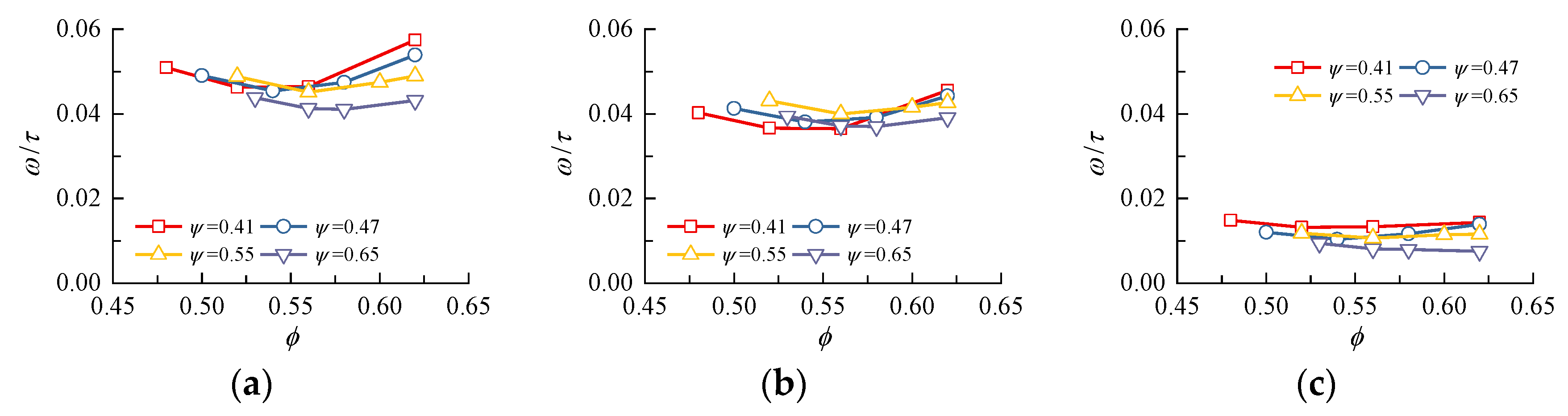
The comparison of the stator passage loss is given in Figure 27, where the losses are divided by the blade solidity just like the rotor. The most striking result about the stator is that the higher loaded design generated a lower total loss in large mass flow rate conditions (see Figure 27a), where the ψ = 0.65 stage exhibited a lower loss level than the other stages. According to Figure 10, the stator solidity of the ψ = 0.65 stage was remarkably higher than that of the other three schemes, thus relieving the loading of every single blade. Inspection of Figure 27b,c indicates that the high-solidity design could effectively control the increase in blade profile loss at high design loadings, whereas the reduction of stator loss stemmed mainly from the endwall region. Note that, although the passage flow would be better organized at higher blade solidity, the total loss of the stator row came from all the blades, which means that the benefit of increasing the solidity was limited.
5. Conclusions
The design and analysis of four well comparable compressor stages were performed to reveal the flow characteristics of the ultrahigh loaded compressor. An experiment was conducted to validate the numerical method, and the calculated flow loss was decomposed on the basis of the flow features to unveil the variation of each part. The main conclusions are drawn below.
- Four compressors were designed under the same flow coefficient with the loading varying from 0.41 to 0.65. The geometrical features of the stages were similar, and the flow fields were organized following the same pattern. The peak efficiency of the four stages was between 0.87 and 0.82, highlighting the state-of-the-art designing ability.
- The blade profile loss dominated the total loss of the rotor passage and played a larger part with the increase in the design loading. The percentage of design-point blade profile loss increased from 69% to 76% when the stage loading was varied from 0.41 to 0.65. The total loss of the rotor blade tended to increase with the increase in the stage pressure rise coefficient, while the increment came mainly from the blade profile loss and the tip leakage loss. The proportion of the blade profile loss was squeezed by the tip leakage loss as Cp increased.
- With the increase in stage pressure rise coefficient, the total loss of the stator first decreased and then increased, while the blade profile loss and the endwall loss held an equal ratio. The blade profile loss in the stator passage was much higher than the losses at the hub and casing corners, whereas the proportion of the blade profile loss increased from 79% to 90% as the design loading changes from 0.41 to 0.65.
- Increasing the solidity reduced the transverse pressure gradient in the blade passage, thereby weakening the tip leakage flow and extending the stage operation range of the ultrahigh loaded compressor. The increase in flow losses in the highly loaded compressor stemmed mainly from the high blade solidity. The selection of solidity should balance between the total loss level and the stage stall margin.
Author Contributions
Conceptualization, X.Y.; methodology, R.W. and X.Y.; validation, G.A.; formal analysis, R.W. and X.Y.; resources, X.Y. and B.L.; data curation, G.A.; writing—original draft preparation, R.W.; writing—review and editing, R.W., X.Y. and B.L.; supervision, X.Y. and B.L.; project administration, B.L.; funding acquisition, X.Y. and B.L. All authors have read and agreed to the published version of the manuscript.
Funding
This investigation was funded by National Natural Science Foundation of China (Grant No. 51790511) and the National Science and Technology Major Project (Grant No. 2017-II-0001-0013).
Institutional Review Board Statement
Not applicable.
Informed Consent Statement
Not applicable.
Data Availability Statement
Not applicable.
Acknowledgments
The authors would like to express their appreciation to Yong Qin for his devotion to the typesetting of this paper.
Conflicts of Interest
The authors declare no conflict of interest.
Nomenclature
| Variables | |
| Cp | Static pressure-rise coefficient |
| DF | Diffusion factor |
| m | Mass flow rate |
| n | Rotating speed |
| T* | Total temperature |
| Umid | Midspan velocity |
| w | Relative velocity |
| βk | Metal angle |
| η | Efficiency |
| π | Total pressure ratio |
| ρ | Density |
| φ | Flow coefficient |
| τ | Solidity |
| ψ | Loading coefficient |
| ω | Loss coefficient |
| Ω | Reaction |
| Subscripts | |
| endwall | Endwall loss |
| hub | Hub loss |
| leakage | Tip leakage loss |
| profile | Blade profile loss |
| tip | Total casing loss |
| tipwall | Casing endwall friction loss |
| tot | Total loss |
References
- Wadia, A.R. Some Advances in Fan and Compressor Aero at GE Aircraft Engines, Lecture; Tsinghua University: Beijing, China, 2005. [Google Scholar]
- Wennerstrom, A.J. Experimental study of a high-throughflow transonic axial compressor stage. J. Eng. Gas Turbines Power 1984, 106, 552–560. [Google Scholar] [CrossRef]
- Koch, C.C. Stalling pressure rise capability of axial flow compressor stages. J. Eng. Power 1981, 103, 645–656. [Google Scholar] [CrossRef]
- Schweitzer, J.K.; Garberoglio, J.E. Maximum loading capability of axial flow compressors. J. Aircr. 1984, 21, 593–600. [Google Scholar] [CrossRef]
- Goodhand, M.N.; Miller, R.J. The impact of real geometries on three-dimensional separations in compressors. J. Turbomach. 2012, 134, 021007. [Google Scholar] [CrossRef]
- Komarov, O.V.; Sedunin, V.A.; Blinov, V.L. Application of optimisation techniques for new high-turning axial compressor profile topology design. In Proceedings of the ASME Turbo 2014, Düsseldorf, Germany, 16–20 June 2014. [Google Scholar] [CrossRef]
- Auchoybur, K.; Miller, R.J. Design of compressor endwall velocity triangles. J. Turbomach. 2017, 139, 061005. [Google Scholar] [CrossRef]
- Yan, T.; Chen, H.; Fang, J.; Yan, P. Research on 3D Design of High-Load Counter-Rotating Compressor Based on Aerodynamic Optimization and CFD Coupling Method. Energies 2022, 15, 4770. [Google Scholar] [CrossRef]
- Benini, E.; Biollo, R. Aerodynamics of swept and leaned transonic compressor-rotors. Appl. Energy 2007, 84, 1012–1027. [Google Scholar] [CrossRef]
- Horlock, J.H.; Denton, J.D. A review of some early design practice using computational fluid dynamics and a current perspective. J. Turbomach. 2005, 127, 5–13. [Google Scholar] [CrossRef]
- Aungier, R.H. Axial-Flow Compressors: A Strategy for Aerodynamic Design and Analysis; ASME Press: New York, NY, USA, 2004. [Google Scholar]
- Schnoes, M.; Nicke, E. Automated calibration of compressor loss and deviation correlations. In Proceedings of the ASME Turbo Expo 2015, Montreal, QC, Canada, 15–19 June 2015. [Google Scholar] [CrossRef]
- Koch, C.C.; Smith, L.H., Jr. Loss sources and magnitudes in axial-flow compressors. J. Eng. Gas Turbines Power 1976, 98, 411–424. [Google Scholar] [CrossRef]
- Wisler, D.C. Loss Reduction in Axial-Flow Compressors Through Low-Speed Model Testing. J. Eng. Gas Turbines Power 1985, 107, 354–363. [Google Scholar] [CrossRef]
- Lakshminarayana, B. Fluid Dynamics and Heat Transfer in Turbomachinery; John Wiley & Sons, Inc.: Hoboken, NJ, USA, 1996. [Google Scholar]
- Howell, A.R. Fluid dynamic of axial compressors. Proc. Inst. Mech. Eng. 1945, 153, 441–452. [Google Scholar] [CrossRef]
- Boyer, K.M.; O’Brien, W.F. An improved streamline curvature approach for off-design analysis of transonic axial compression systems. J. Turbomach. 2003, 125, 475–481. [Google Scholar] [CrossRef]
- Denton, J.D. Loss mechanisms in turbomachines. J. Turbomach. 1993, 115, 621–656. [Google Scholar] [CrossRef]
- Saito, S.; Furukawa, M.; Yamada, K.; Watanable, K.; Matsuoka, A.; Niwa, N. Mechanisms and quantitative evaluation of flow loss generation in a multi-stage transonic axial compressor. In Proceedings of the ASME Turbo Expo 2019, Phoenix, AZ, USA, 17–21 June 2019. [Google Scholar] [CrossRef]
- To, H.-O.; Miller, R. The effect of aspect ratio on compressor performance. J. Turbomach. 2019, 141, 081011. [Google Scholar] [CrossRef]
- Zhang, H.D.; Wu, Y.; Li, Y.H. Evaluation of RANS turbulence models in simulating the corner separation of a high-speed compressor cascade. Eng. Appl. Comp. Fluid 2015, 9, 477–489. [Google Scholar] [CrossRef]
- Liu, J.-X.; Yang, F.-S.; Huo, T.-Q.; Deng, J.-Q.; Zhang, Z.-X. Analysis of Impact of a Novel Combined Casing Treatment on Flow Characteristics and Performance of a Transonic Compressor. Energies 2022, 15, 5066. [Google Scholar] [CrossRef]
- Cao, Z.Y.; Song, C.; Gao, X.; Zhang, X.; Zhang, F.; Liu, B. Effects of pulsed endwall air injection on corner separation and vortical flow of a compressor cascade. Eng. Appl. Comp. Fluid 2022, 16, 879–903. [Google Scholar] [CrossRef]
- Liu, B.J.; Qiu, Y.; An, G.F.; Yu, X.J. Utilization of zonal method for five-hole probe measurements of complex axial compressor flows. J. Fluids Eng. 2020, 142, 061504. [Google Scholar] [CrossRef]
- Liu, B.J.; An, G.F.; Yu, X.J.; Zhang, Z.B. Experimental investigation of the effect of rotor tip gaps on 3D separating flows inside the stator of a highly loaded compressor stage. Exp. Therm. Fluid Sci. 2016, 75, 96–107. [Google Scholar] [CrossRef] [Green Version]
Figure 1.
Geometry configuration and mesh for the compressor stage (ψ = 0.41).
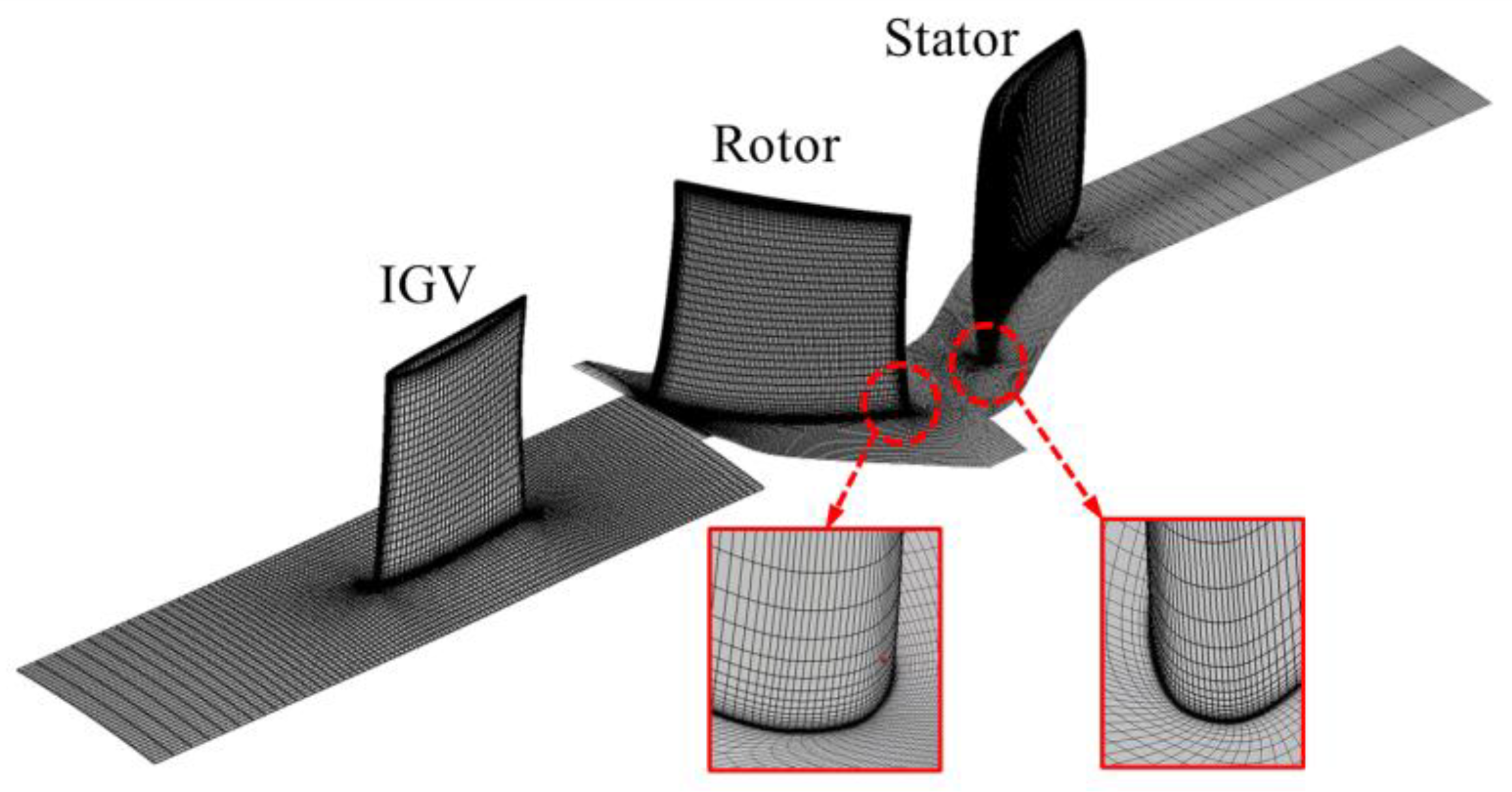
Figure 2.
Comparison of stage characteristic for different grid schemes: (a) design point; (b) near-stall point.
Figure 2.
Comparison of stage characteristic for different grid schemes: (a) design point; (b) near-stall point.
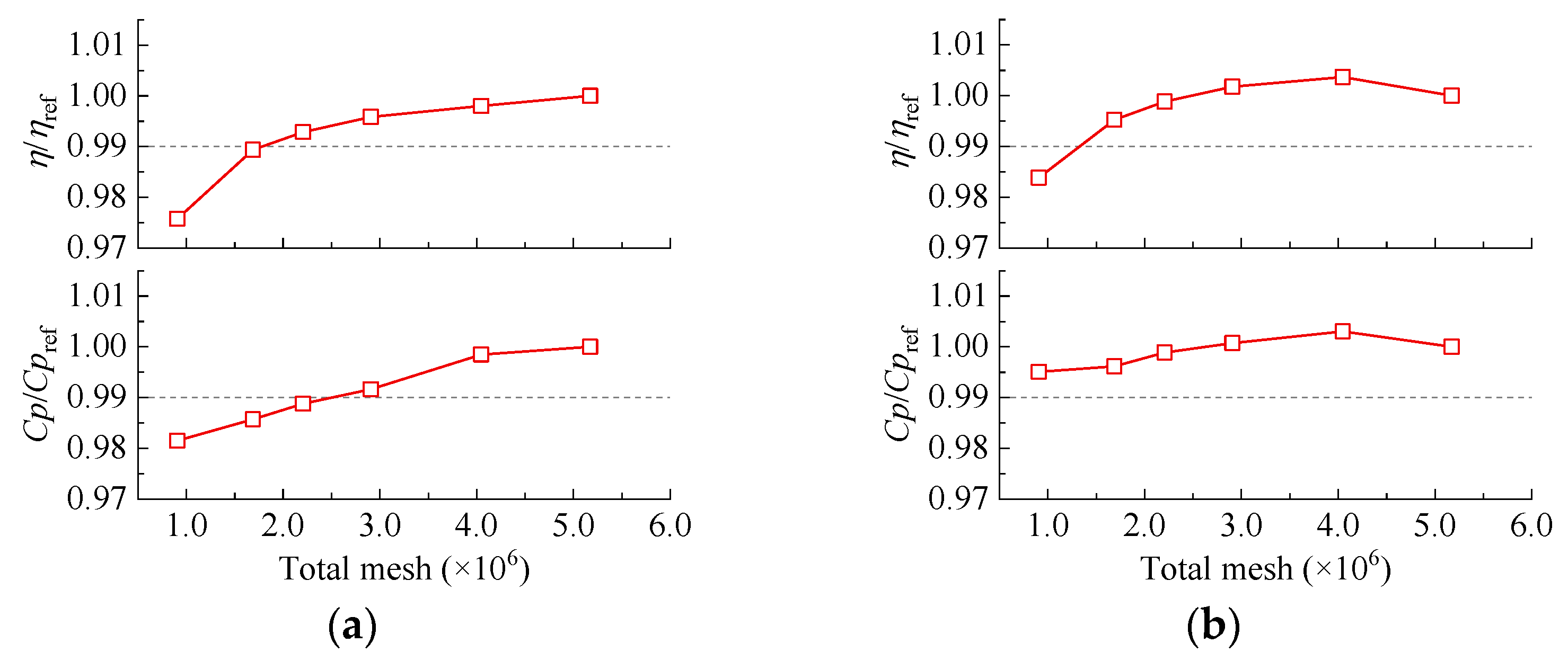
Figure 3.
The experimental rig: (a) multifunctional vertical axial compressor test facility; (b) measurement planes; (c) 3D-printed blade; (d) the L-shaped five-hole probe.
Figure 3.
The experimental rig: (a) multifunctional vertical axial compressor test facility; (b) measurement planes; (c) 3D-printed blade; (d) the L-shaped five-hole probe.
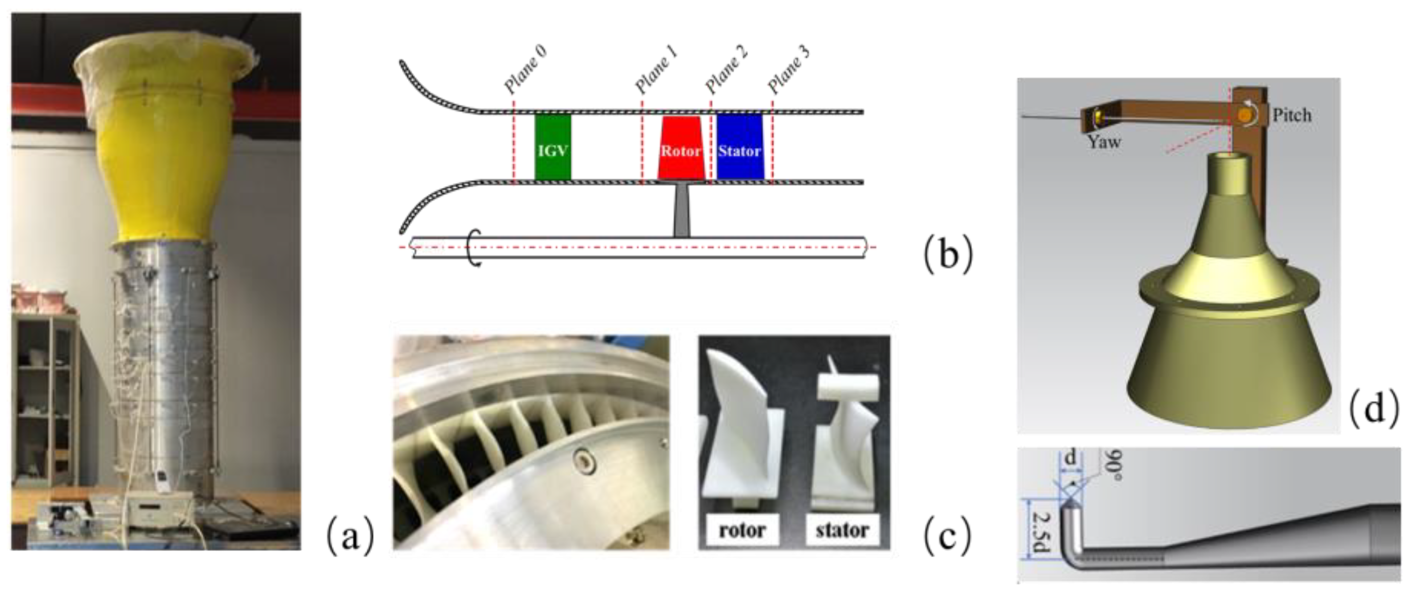
Figure 4.
The arrangement of measurement points at the rotor and stator outlet.
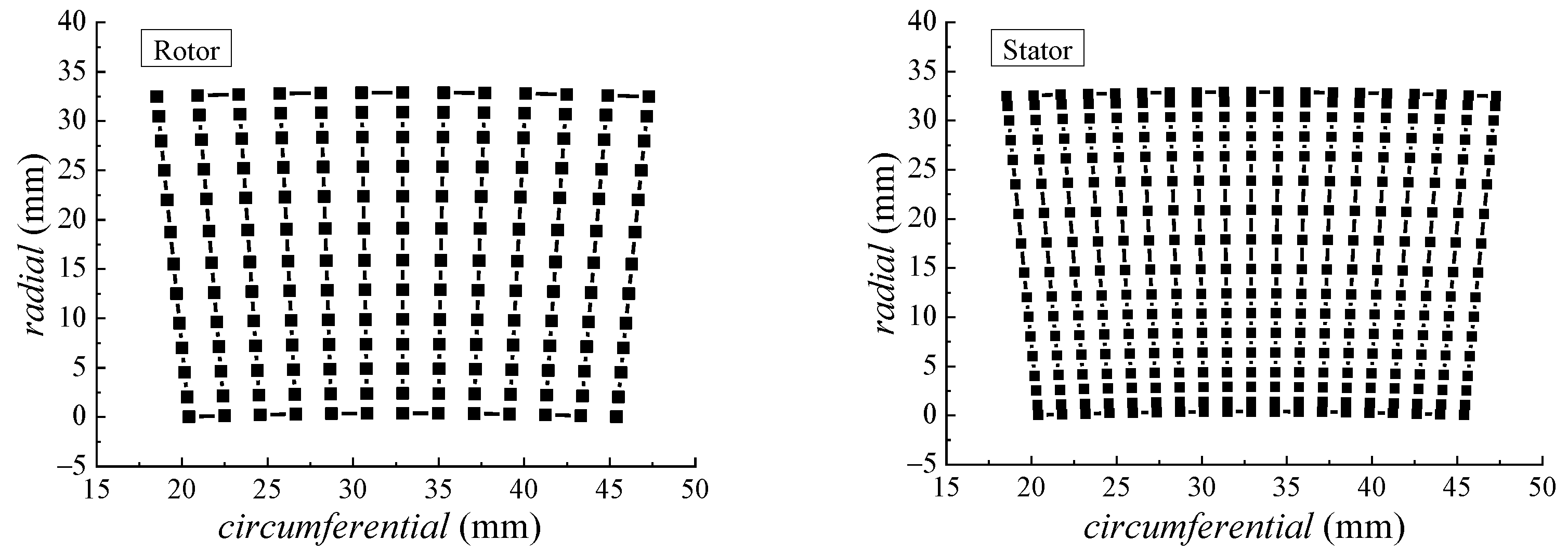
Figure 5.
Comparison of stage characteristics between the experiment and numerical simulation.
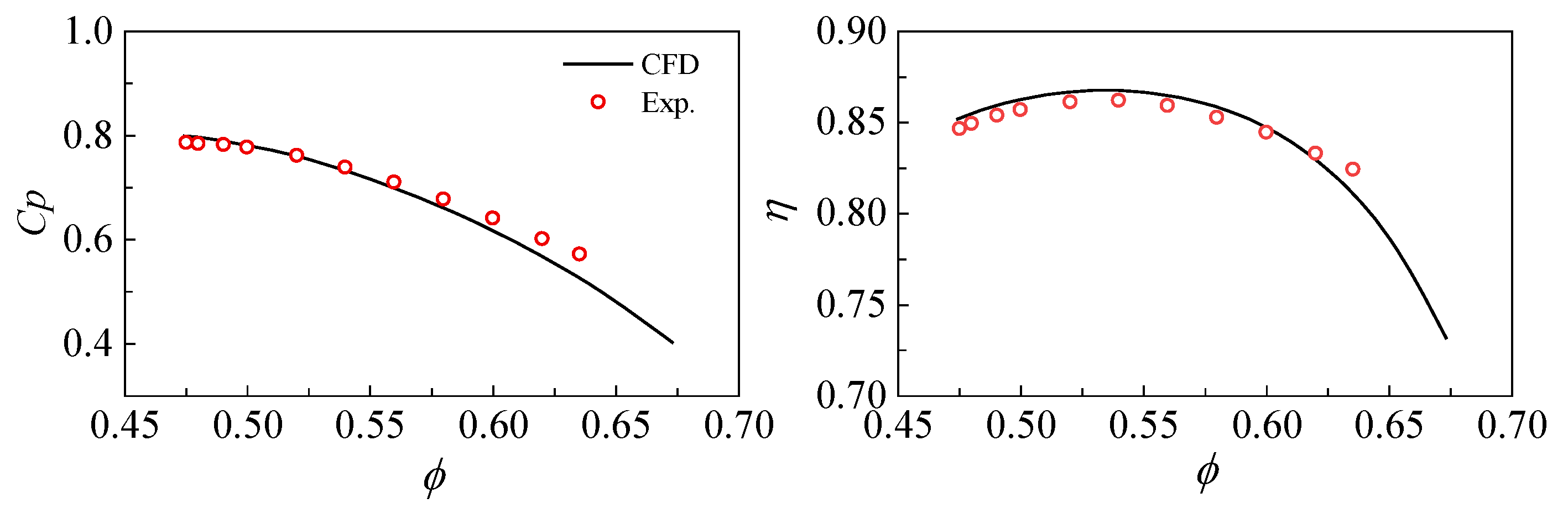
Figure 6.
Comparison of rotor and stator flow angle between the experiment and numerical simulation: (a) rotor; (b) stator.
Figure 6.
Comparison of rotor and stator flow angle between the experiment and numerical simulation: (a) rotor; (b) stator.
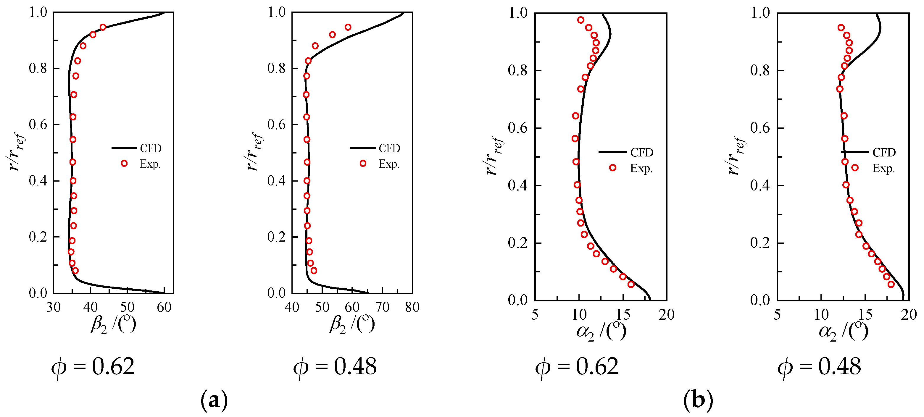
Figure 7.
Comparison of rotor and stator loss between the experiment and numerical simulation: (a) rotor; (b) stator.
Figure 7.
Comparison of rotor and stator loss between the experiment and numerical simulation: (a) rotor; (b) stator.
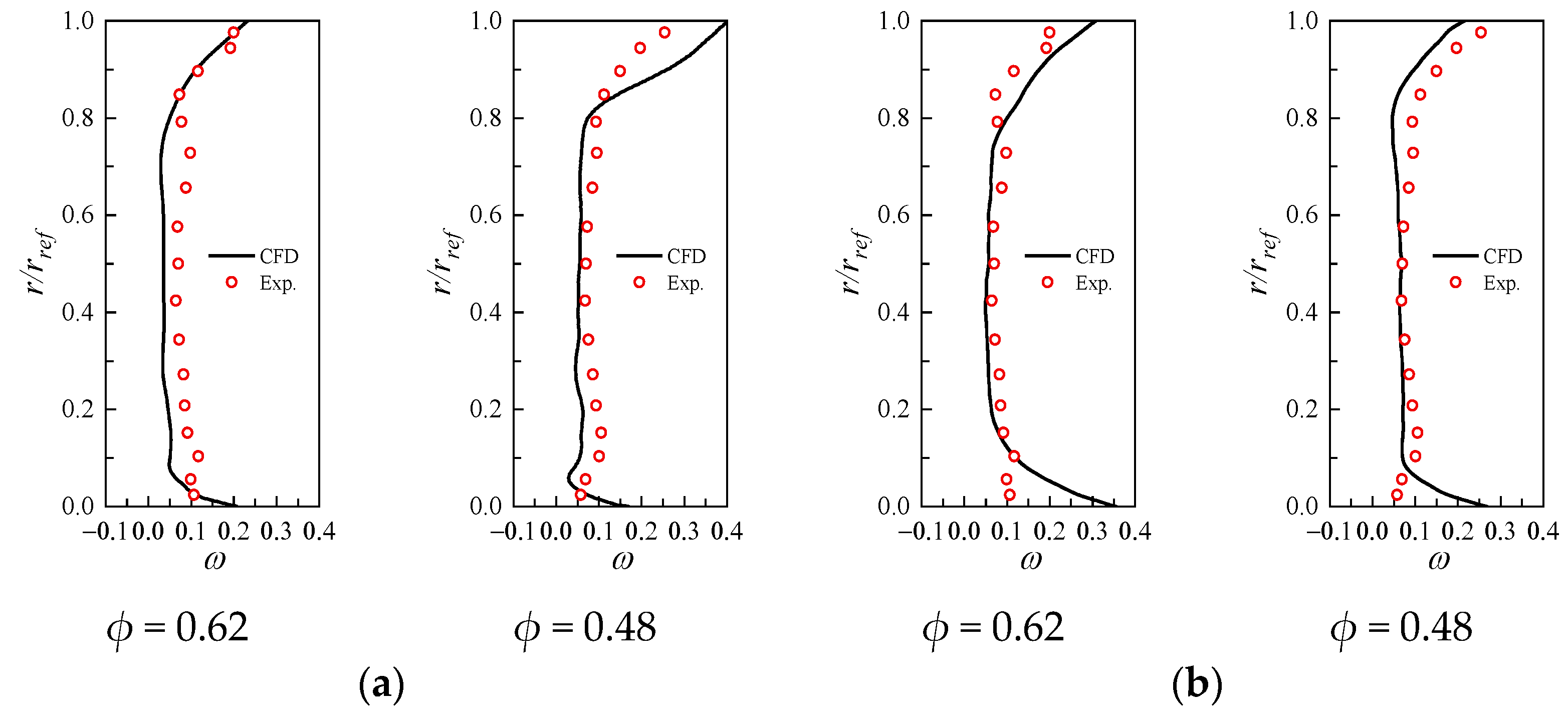
Figure 8.
Geometric configuration of the four compressor stages.

Figure 9.
Comparison of design parameters for the four compressor stages: rotor.

Figure 10.
Comparison of design parameters for the four compressor stages: stator.
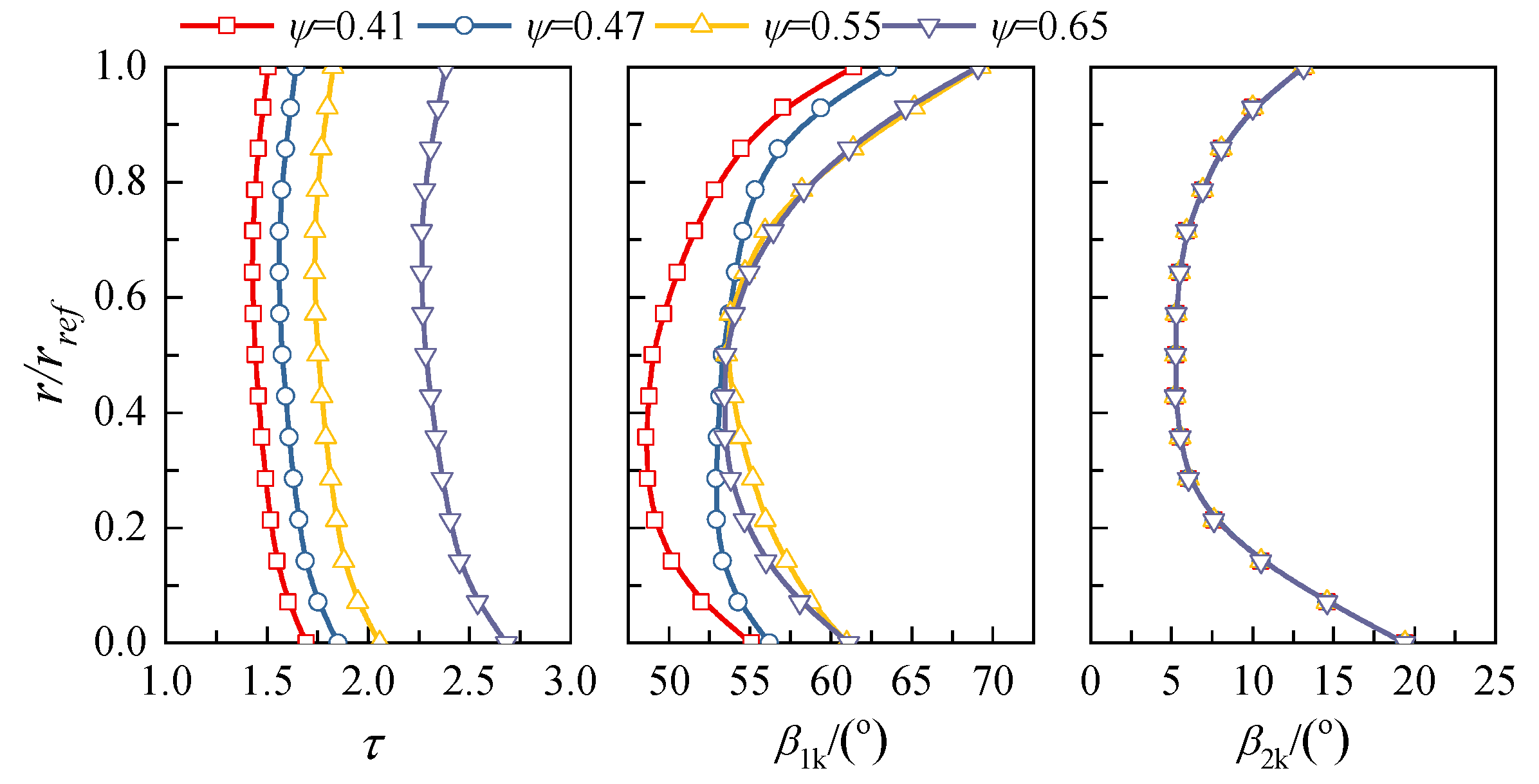
Figure 11.
Stage pressure-rise coefficient and efficiency.
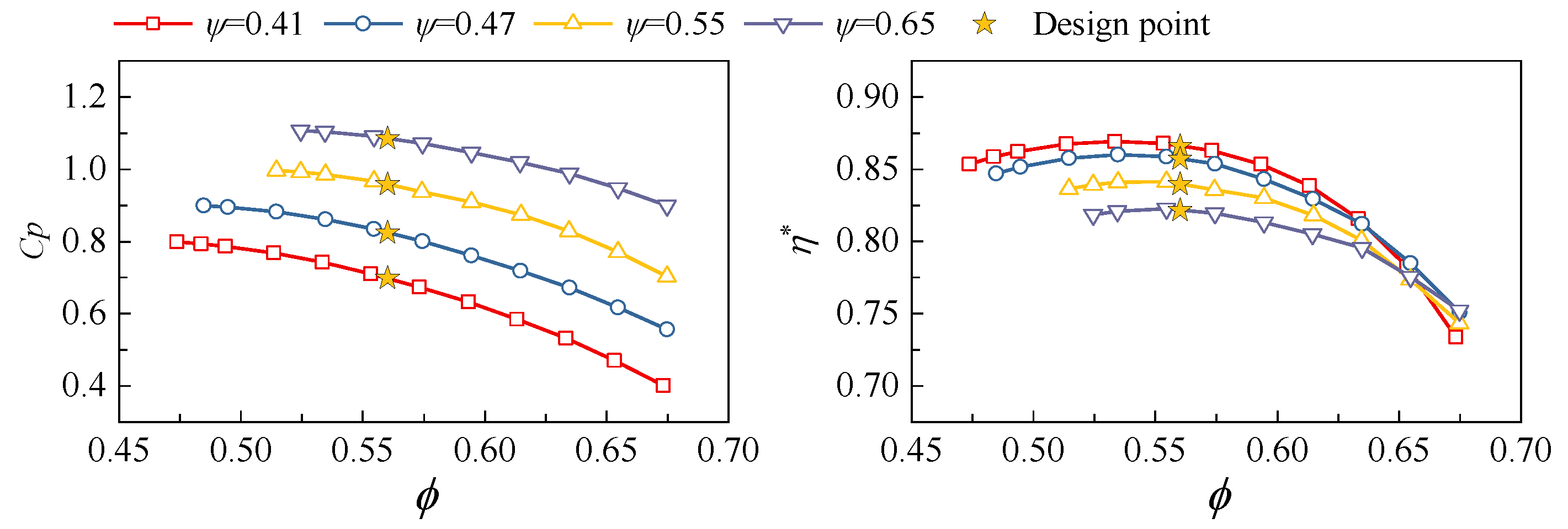
Figure 12.
Radial characteristic for different compressor stages: design point.

Figure 13.
Spanwise aerodynamic performance for different compressor stages: near-stall point.

Figure 14.
Loss decomposition process for the compressor stages: (a) rotor; (b) stator.
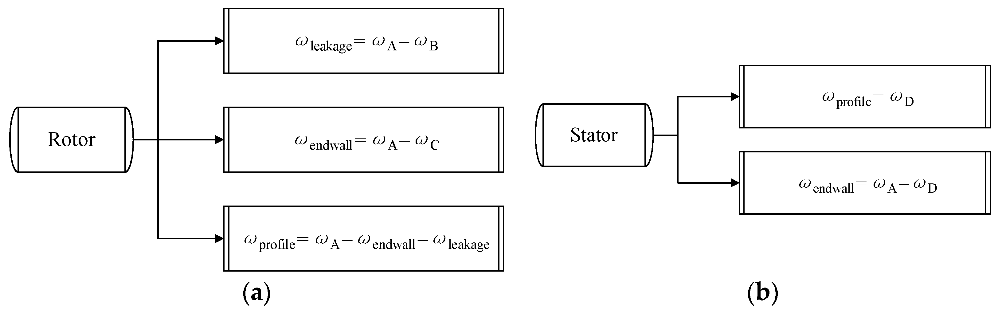
Figure 15.
Demonstration of the loss decomposition results: (a) rotor loss decomposition; (b) stator loss decomposition.
Figure 15.
Demonstration of the loss decomposition results: (a) rotor loss decomposition; (b) stator loss decomposition.
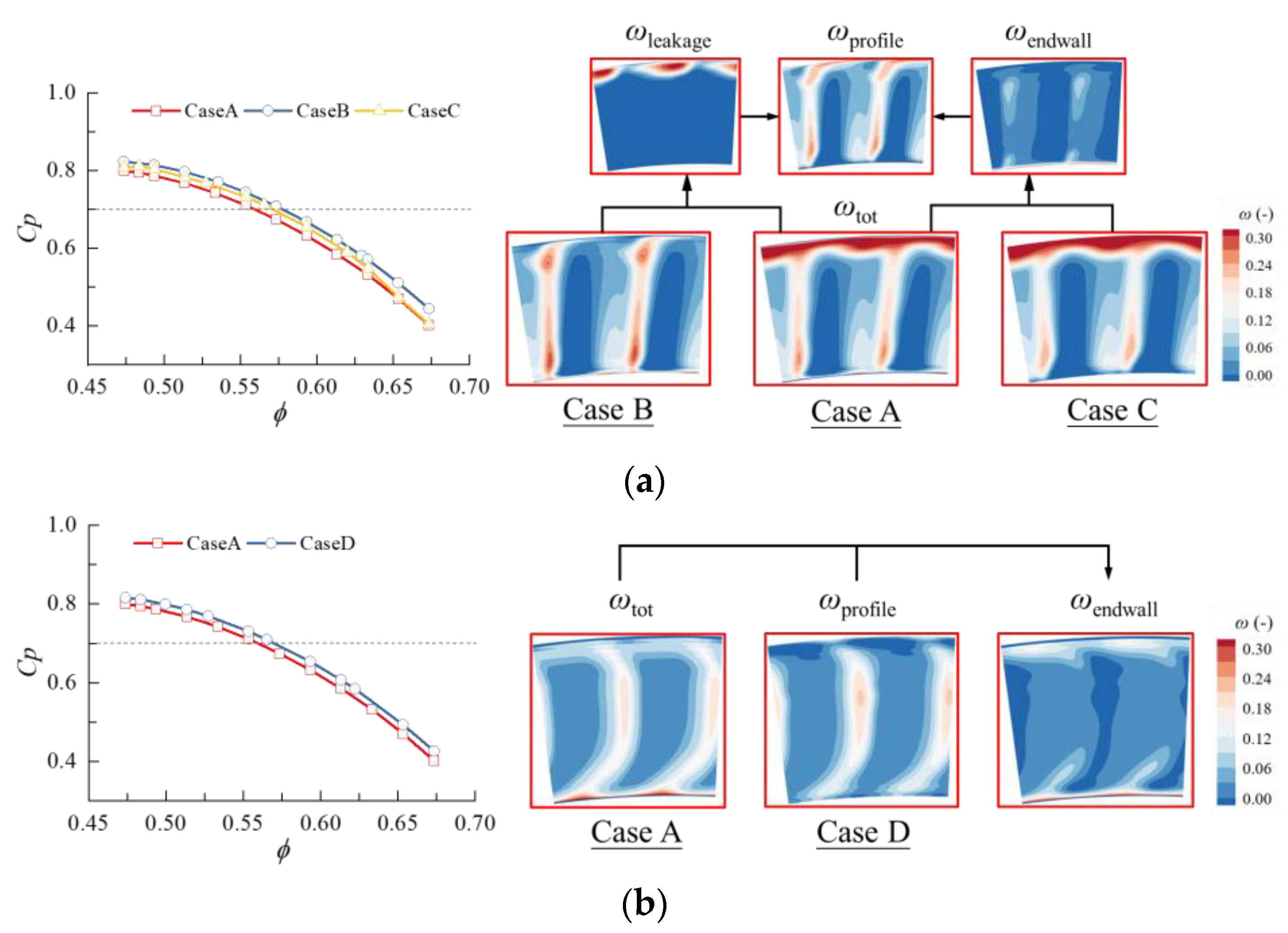
Figure 16.
The comparison between the different loss decomposition methods.

Figure 17.
The distribution of rotor static pressure rise coefficient at midspan: (a) design condition; (b) near stall condition.
Figure 17.
The distribution of rotor static pressure rise coefficient at midspan: (a) design condition; (b) near stall condition.
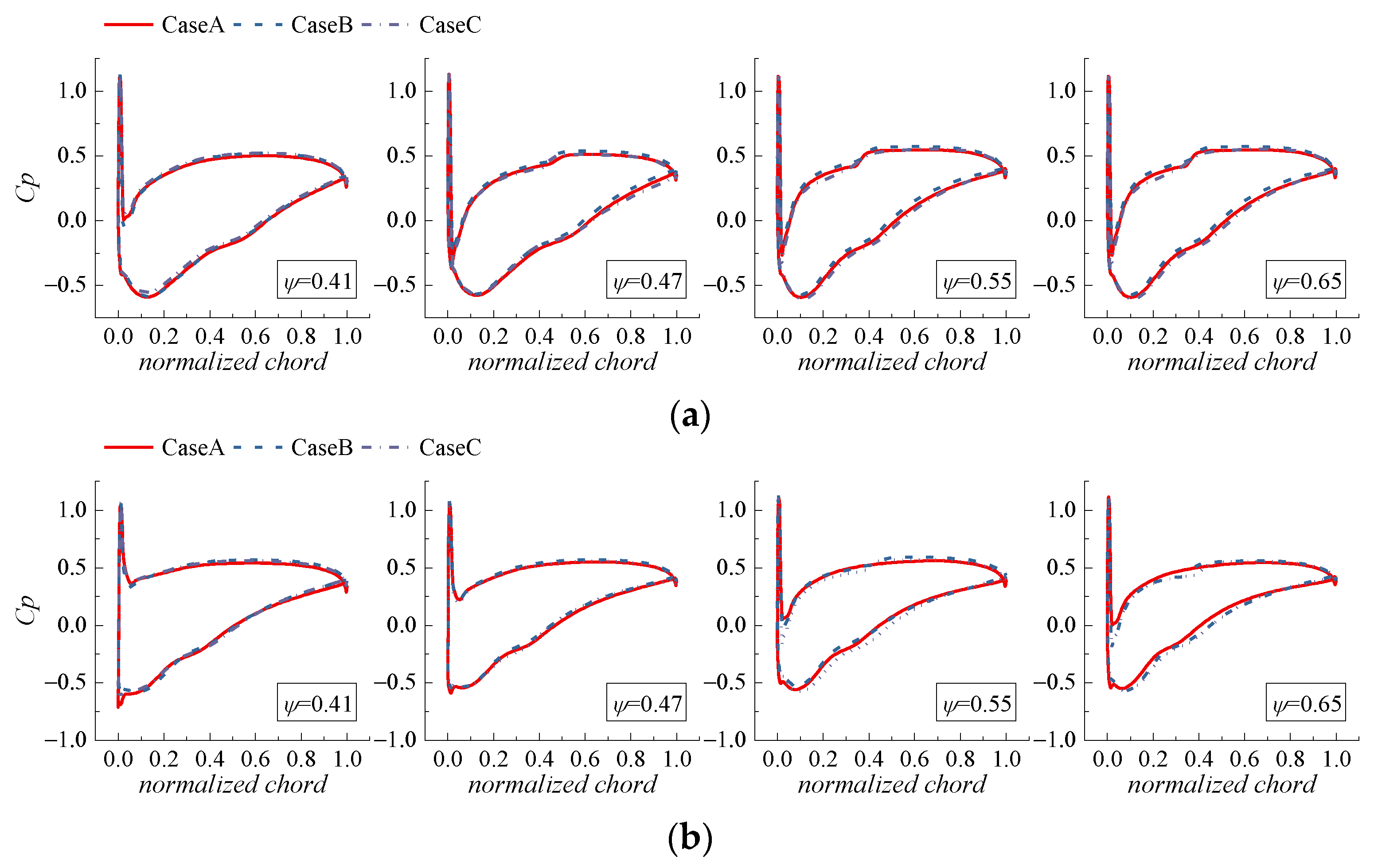
Figure 18.
The distribution of stator static pressure rise coefficient at midspan at the near-stall condition: (a) design condition; (b) near stall condition.
Figure 18.
The distribution of stator static pressure rise coefficient at midspan at the near-stall condition: (a) design condition; (b) near stall condition.
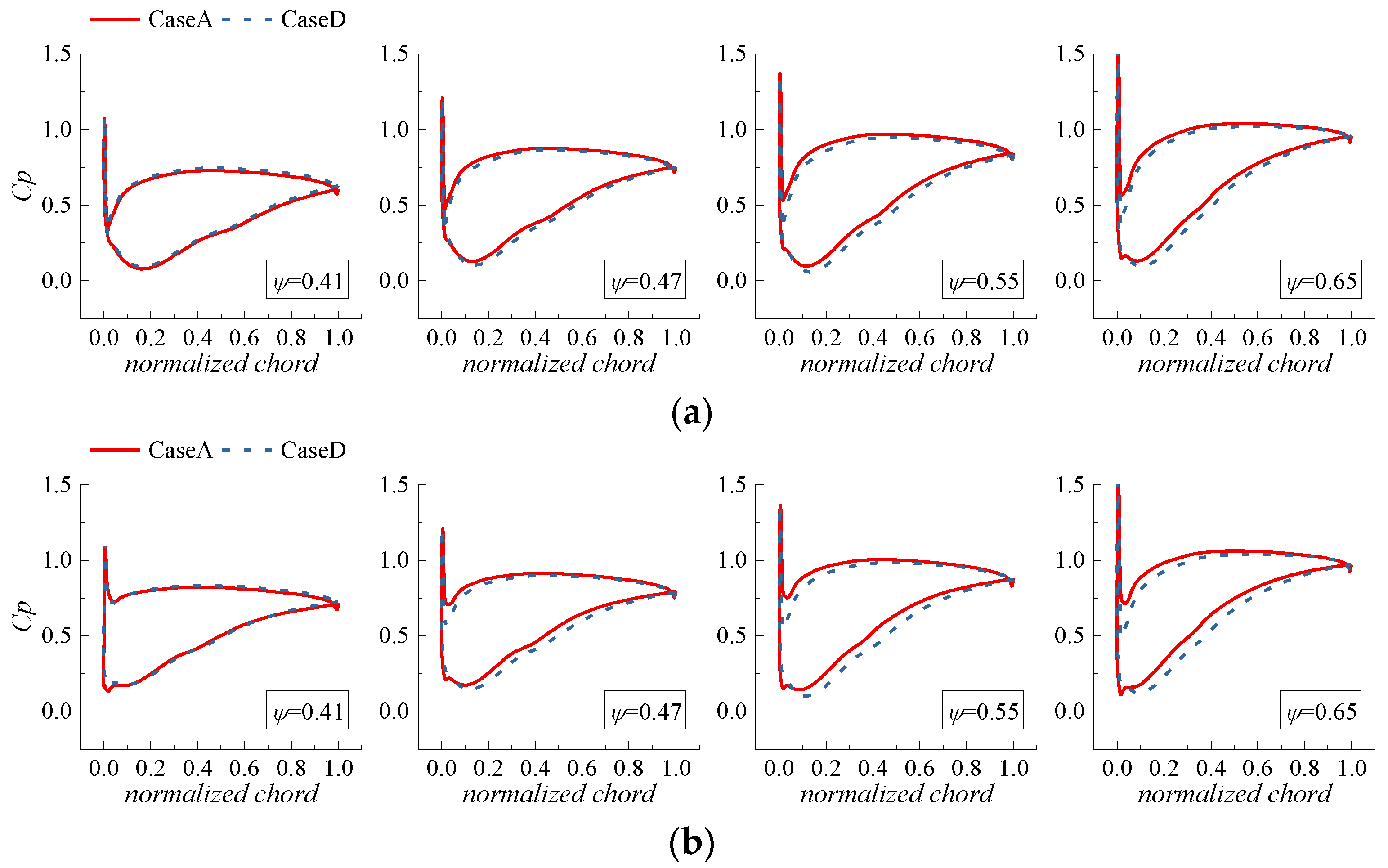
Figure 19.
Decomposition of the total pressure loss along the radial direction (ψ = 0.41, design point): (a) rotor; (b) stator.
Figure 19.
Decomposition of the total pressure loss along the radial direction (ψ = 0.41, design point): (a) rotor; (b) stator.

Figure 20.
The distribution of total pressure loss at rotor outlet for the design point: (a) ψ = 0.41; (b) ψ = 0.47; (c) ψ = 0.55; (d) ψ = 0.65.
Figure 20.
The distribution of total pressure loss at rotor outlet for the design point: (a) ψ = 0.41; (b) ψ = 0.47; (c) ψ = 0.55; (d) ψ = 0.65.

Figure 21.
The distribution of pitch-averaged endwall loss for the rotor blade: (a) ψ = 0.41; (b) ψ = 0.47; (c) ψ = 0.55; (d) ψ = 0.65.
Figure 21.
The distribution of pitch-averaged endwall loss for the rotor blade: (a) ψ = 0.41; (b) ψ = 0.47; (c) ψ = 0.55; (d) ψ = 0.65.
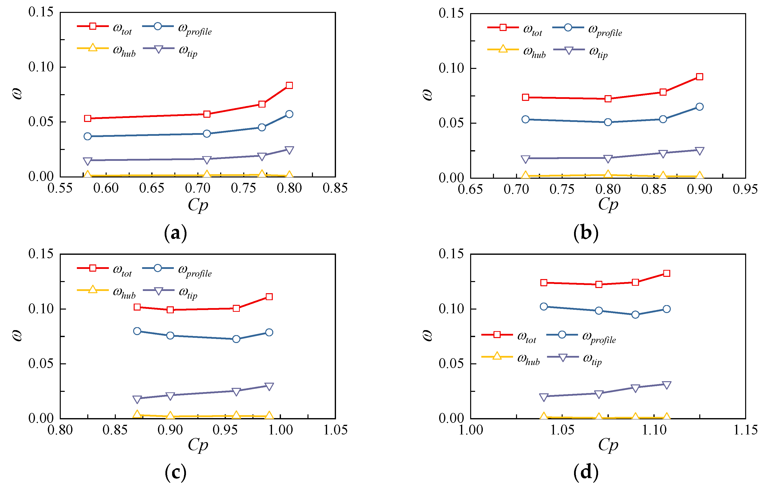
Figure 22.
The composition of loss for the rotor blade: (a) ψ = 0.41; (b) ψ = 0.47; (c) ψ = 0.55; (d) ψ = 0.65.
Figure 22.
The composition of loss for the rotor blade: (a) ψ = 0.41; (b) ψ = 0.47; (c) ψ = 0.55; (d) ψ = 0.65.
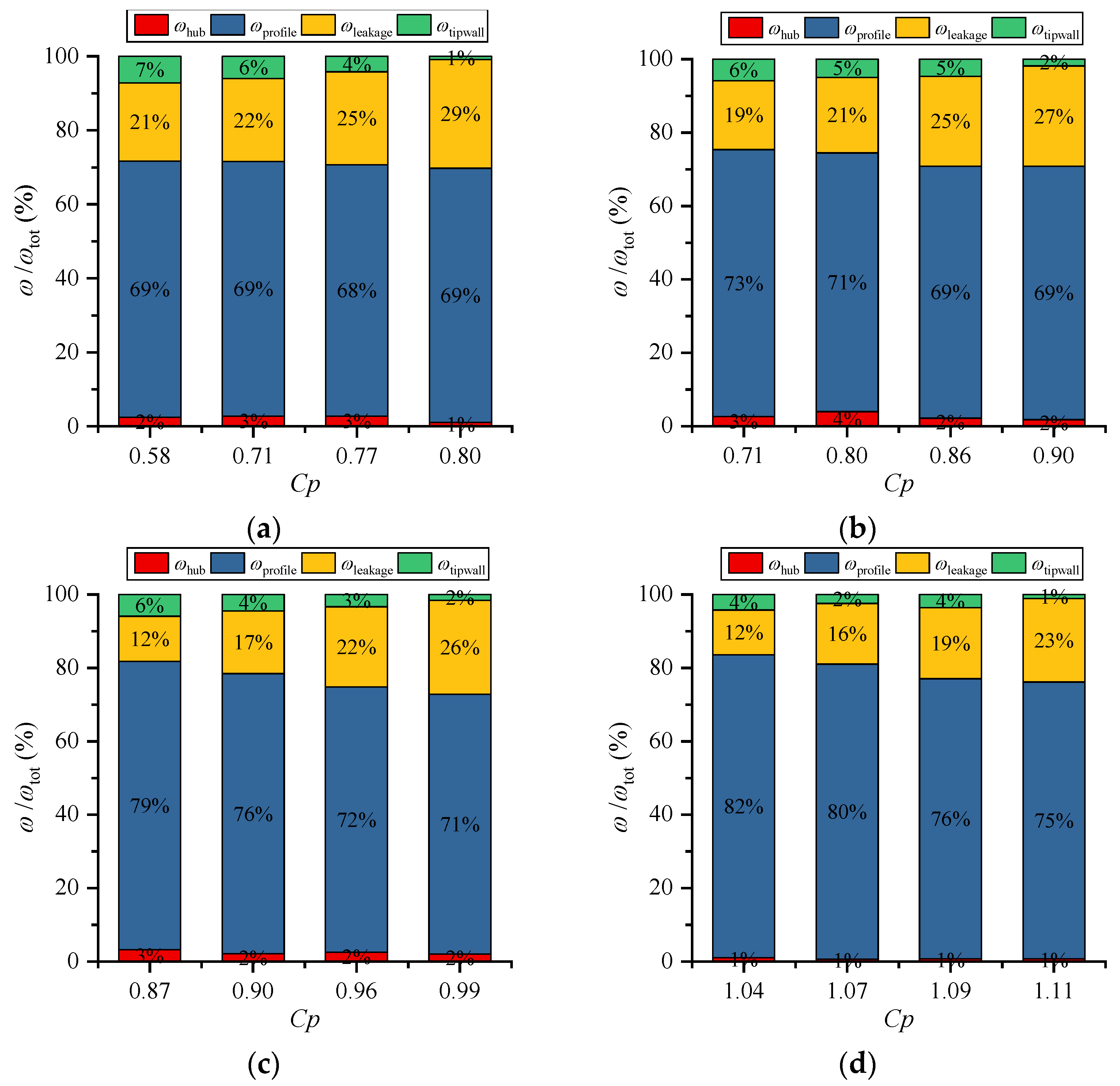
Figure 23.
The distribution of total pressure loss at stator outlet for the design point: (a) ψ = 0.41; (b) ψ = 0.47; (c) ψ = 0.55; (d) ψ = 0.65.
Figure 23.
The distribution of total pressure loss at stator outlet for the design point: (a) ψ = 0.41; (b) ψ = 0.47; (c) ψ = 0.55; (d) ψ = 0.65.
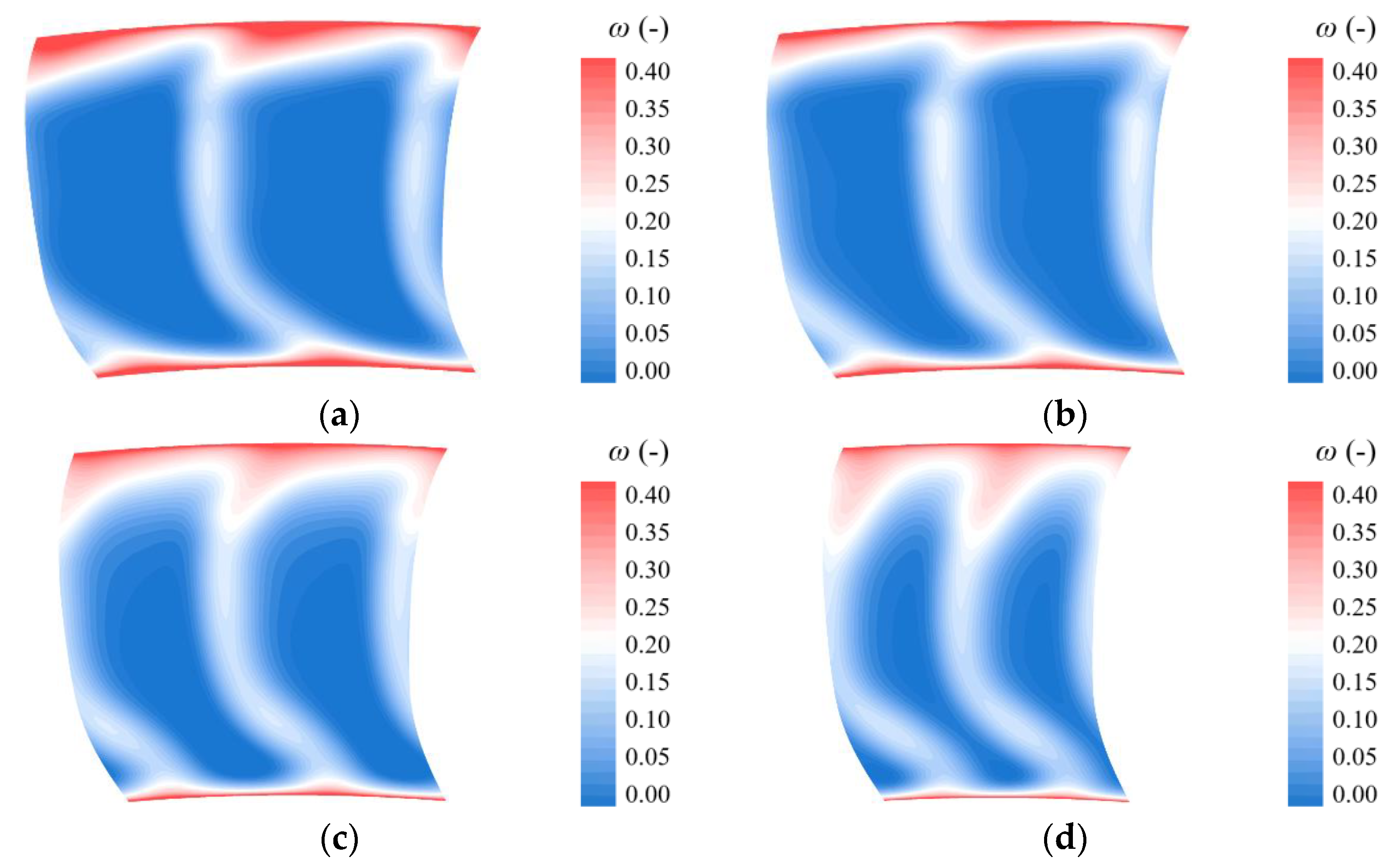
Figure 24.
The distribution of pitch-averaged endwall loss for the stator blade: (a) ψ = 0.41; (b) ψ = 0.47; (c) ψ = 0.55; (d) ψ = 0.65.
Figure 24.
The distribution of pitch-averaged endwall loss for the stator blade: (a) ψ = 0.41; (b) ψ = 0.47; (c) ψ = 0.55; (d) ψ = 0.65.
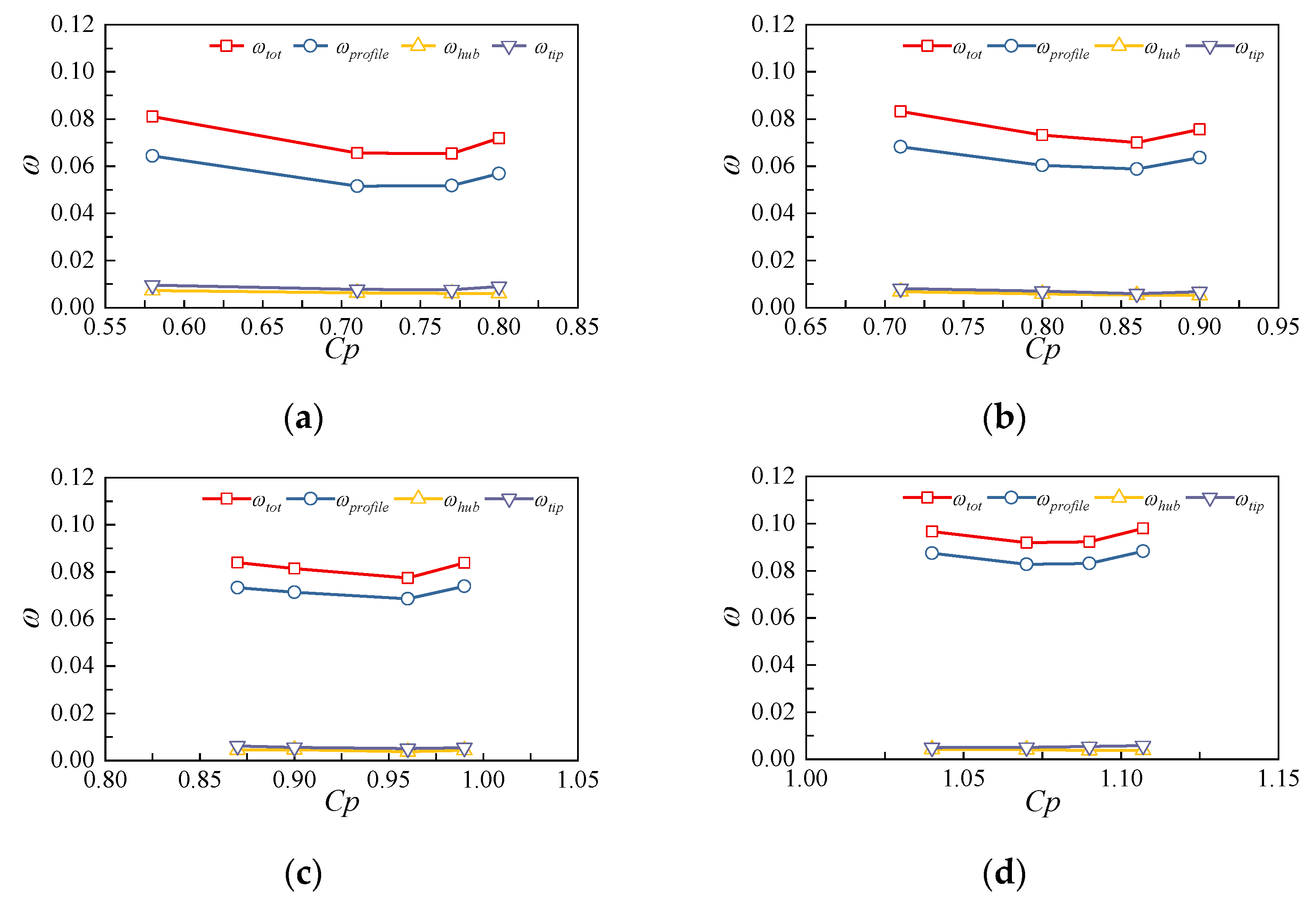
Figure 25.
The composition of loss for the stator blade: (a) ψ = 0.41; (b) ψ = 0.47; (c) ψ = 0.55; (d) ψ = 0.65.
Figure 25.
The composition of loss for the stator blade: (a) ψ = 0.41; (b) ψ = 0.47; (c) ψ = 0.55; (d) ψ = 0.65.
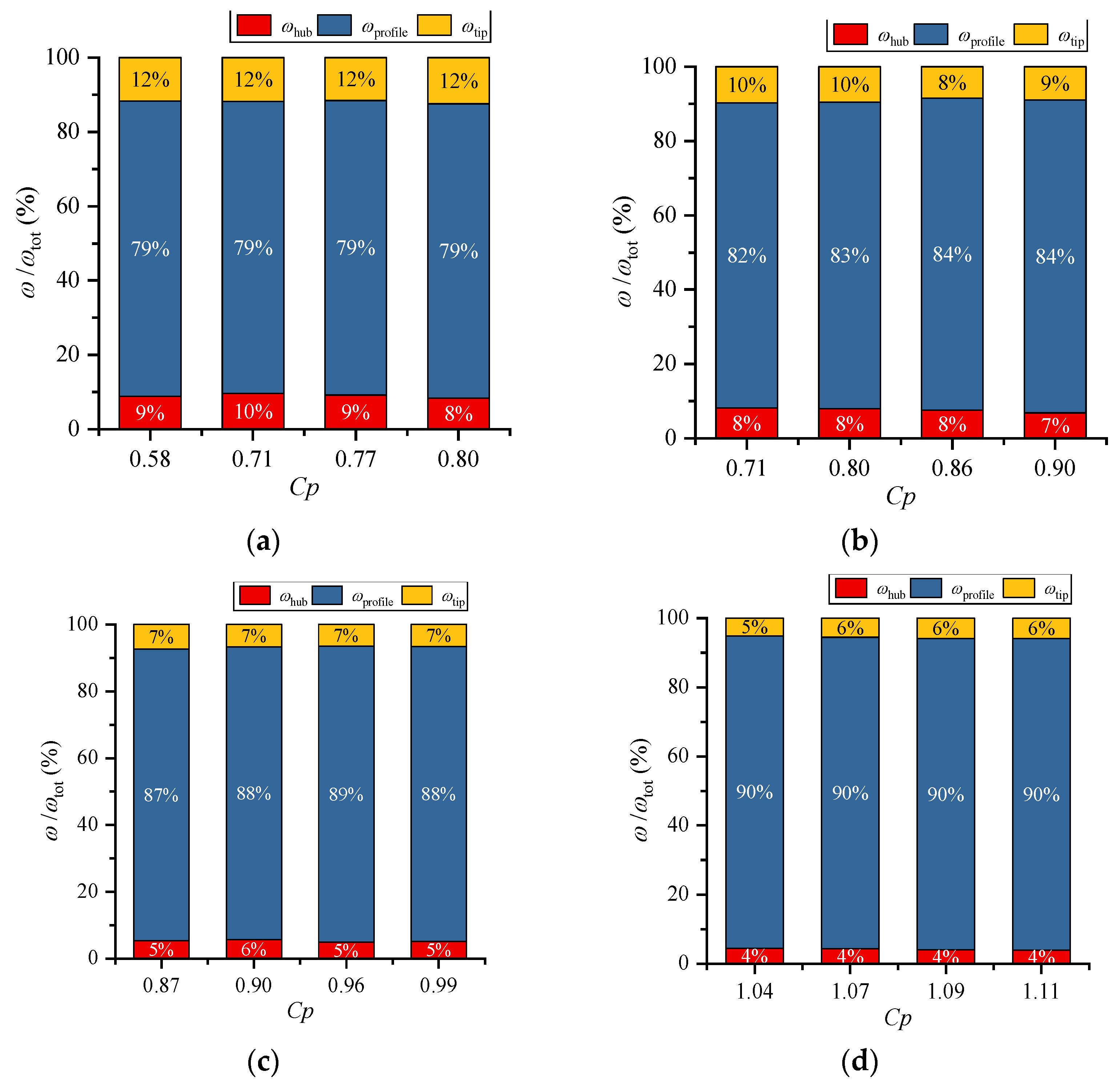
Figure 26.
The comparison of rotor loss between different design schemes: (a) total loss; (b) blade profile loss; (c) tip leakage loss.
Figure 26.
The comparison of rotor loss between different design schemes: (a) total loss; (b) blade profile loss; (c) tip leakage loss.
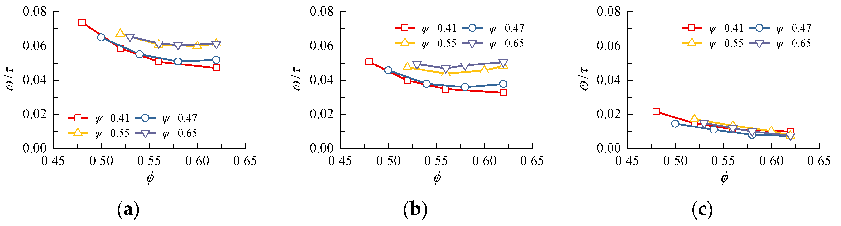
Figure 27.
The comparison of stator loss between different design schemes: (a) total loss; (b) blade profile loss; (c) endwall loss.
Figure 27.
The comparison of stator loss between different design schemes: (a) total loss; (b) blade profile loss; (c) endwall loss.

Table 1.
Design parameters for different compressor stages.
| Stage 1 | Stage 2 | Stage 3 | Stage 4 | |
|---|---|---|---|---|
| Loading coefficient ψ (-) | 0.41 | 0.47 | 0.55 | 0.65 |
| Pressure rise coefficient Cp (-) | 0.71 | 0.83 | 0.97 | 1.09 |
| Stage efficiency (rotor + stator) η (-) | 0.86 | 0.86 | 0.84 | 0.82 |
| Flow coefficient φ (-) | 0.56 | |||
| Tip diameter (m) | 0.25 | |||
| Hub-to-tip ratio (-) | 0.85 | |||
| Rotating speed n (rpm) | 2400 | |||
Table 2.
Grid parameters for the grid independence study.
| IGV Grid (×106) | Rotor Grid (×106) | Spanwise Grid in the Rotor Shroud Gap | Stator Grid (×106) | |
|---|---|---|---|---|
| Mesh 1 | 0.85 | 0.43 | 13 | 0.34 |
| Mesh 2 | 0.84 | 21 | 0.60 | |
| Mesh 3 | 1.14 | 29 | 0.76 | |
| Mesh 4 | 1.51 | 37 | 1.00 | |
| Mesh 5 | 1.96 | 41 | 1.49 | |
| Mesh 6 | 2.53 | 41 | 1.89 |
Table 3.
Calculation scheme for the loss decomposition.
| Case A | Case B | Case C | Case D | |
|---|---|---|---|---|
| Tip clearance | 1.5% span | 0 | 1.5% span | 1.5% span |
| Hub and shroud walls: rotor | non-slip wall | non-slip wall | slip wall | non-slip wall |
| Hub and shroud walls: stator | non-slip wall | non-slip wall | non-slip wall | slip wall |
Publisher’s Note: MDPI stays neutral with regard to jurisdictional claims in published maps and institutional affiliations. |
© 2022 by the authors. Licensee MDPI, Basel, Switzerland. This article is an open access article distributed under the terms and conditions of the Creative Commons Attribution (CC BY) license (https://creativecommons.org/licenses/by/4.0/).
Share and Cite
MDPI and ACS Style
Wang, R.; Yu, X.; Liu, B.; An, G. Effects of Loading Level on the Variation of Flow Losses in Subsonic Axial Compressors. Energies 2022, 15, 6251. https://doi.org/10.3390/en15176251
AMA Style
Wang R, Yu X, Liu B, An G. Effects of Loading Level on the Variation of Flow Losses in Subsonic Axial Compressors. Energies. 2022; 15(17):6251. https://doi.org/10.3390/en15176251
Chicago/Turabian StyleWang, Ruoyu, Xianjun Yu, Baojie Liu, and Guangfeng An. 2022. "Effects of Loading Level on the Variation of Flow Losses in Subsonic Axial Compressors" Energies 15, no. 17: 6251. https://doi.org/10.3390/en15176251
Note that from the first issue of 2016, this journal uses article numbers instead of page numbers. See further details here.