
Ellipsoidal Design of Robust Stabilization for Markov Jump Power Systems under Normal and Contingency Conditions


1
Department of Electrical Power Engineering, Faculty of Engineering, Cairo University, Giza 12613, Egypt
2
Department of Electrical and Electronics Engineering, Istanbul Esenyurt University, Istanbul 34517, Turkey
3
Energy and Renewable energy Department, Faculty of Engineering, Egyptian Chinese University, Cairo 11724, Egypt
4
Department of Engineering, Niccolò Cusano University, 00166 Rome, Italy
*
Author to whom correspondence should be addressed.
Energies 2022, 15(19), 7249; https://doi.org/10.3390/en15197249
Submission received: 30 August 2022
/
Revised: 18 September 2022
/
Accepted: 28 September 2022
/
Published: 2 October 2022
(This article belongs to the Topic Power System Modeling and Control, 2nd Volume)
Abstract
:The essential prerequisites for secure customer service are power system stability and reliability. This work shows how to construct a robust switching control for studying power system load changes using an invariant ellipsoid method. Furthermore, the suggested control ensures stability when the system is subjected to random stochastic external disturbances, and functions randomly in two conditions: normal and contingency. The extreme (least) reliability state is chosen as the most severe scenario (corresponding to a transmission line outage). As a two-state Markov random chain, the transition probabilities are utilized to simulate the switching between normal and contingency modes (or processes). To characterize the dynamics of the studied system, a stochastic mathematical model is developed. The effect of stochastic disturbances and random normal/contingency operations is taken into account during the design stage. For a stochastic power system, a novel excitation control is designed. The attractive ellipsoid approach and linear matrix inequalities (LMIs) optimization are used to build the best two-controller gains. Therefore, the proposed modeling/design technique can be employed for the power system under load changes, stochastic topological changes, and random disturbances. Finally, the system’s random dynamics simulation indicates the effectiveness of the designed control law.
1. Introduction
For economic reasons, modern power systems operate close to their stability limits which are rotor angle stability, frequency stability, and voltage stability [1]. Angle instability is concerned with the loss of synchronism in generators. Power systems are complex nonlinear systems that are subjected to low-frequency natural oscillations that can cause generators to lose synchronism and system separation. The large loop gain of the fast-acting automated voltage regulator (AVR) is responsible for inadequate oscillation damping [1]. Excitation control and power system stabilizers (PSSs) are commonly used to ensure system stability and dampen oscillations [2,3,4]. Operating point changes, topological changes (e.g., transmission line failure/repair), and other factors can all contribute to parametric uncertainty. Random wind speed fluctuations, for example, create changes in phase conductor separation. As a result, there is a random variation in line reactance (which enters the state-space model).
There are different ways to tackle load and transmission line uncertainty. For example, Ref. [4] devised a robust fuzzy-based PSS method, Ref. [5] used particle swarm optimization (PSO) to design robust PSS, and Ref. [6] utilized an improved nature-inspired technique called sunflower optimization algorithm (SFO) to design robust multi-machine PSSs optimally. Furthermore, Ref. [7] used the resilient decentralized control technique to address the PSS design scheme for parameter uncertainty in both the plant and controller. The reliable control refers to stabilizers that tackle more severe cases, such as component failure. Ref. [8] describes the PSS/governor control of a reliable power system. Stability is maintained whether one or both controllers are sound.
To examine the load–frequency control for frequency stability, many control strategies have been employed (see refs. [9,10,11,12] and the references therein). A reliable load–frequency control with parameter uncertainty was examined in [9]. For connected power systems that take time delays into account, the H∞ load–frequency control has been investigated in [12]. Additionally, a sliding-mode control has been developed [13]. Through the event-triggered data transmission technique, an H∞ memory-based load–frequency control for deception attacks on power grids is examined [14].
In reality, the dynamical system model may undergo abrupt changes as a result of component failure or repair, environmental disturbances, abrupt changes in subsystem linkages, and other reasons [15,16]. These variations can be modeled using a Markov random chain or process because they are stochastic. Markov jump systems are base systems with these jumping properties [17]. These features cause the topology of power systems to rapidly change, and it has been said that this topology flips between finite modes modeled as a Markov process [18]. Markov jump-based power systems (MJPSs) have been thoroughly investigated in the past as they offer a better description of systems with random fluctuations or structural changes [18,19,20]. For instance, sudden and unpredictable changes in power grid stabilization are discussed in [19]. Additionally, Ref. [20] used actuator failures and rapid changes to show how MJPSs’ fault-tolerant control architecture works. A series of lightning strikes and the robust control of power systems under stochastic external disturbances are presented in [21], along with circuit breaker open/auto-reclose. The stability of discrete-time power systems vulnerable to arbitrary rapid changes in power systems is examined in [22]. Notably, only roughly 7% of faults are permanent, whereas 80% of faults are transient. Refer to [21,22] for more information on transient faults connected to the circuit breaker protection system’s auto-reclosure. Unlike [21,22], the last problem is solved using the asynchronous control, as given in [23].
The power system must be stable under diverse operating situations to ensure supply security. It should also be safeguarded in the event of any likely contingency. Contingency analysis examines the consequences of a single power system component failure on power system operating conditions when the single component (e.g., transmission line, power transformer, generating unit) is withdrawn from the system. It is worth noting that transmission lines are the most vulnerable to lightning strikes, which could result in faults and subsequent circuit breaker (on/off) switching. This condition necessitates a line failure/repair reliability assessment. The rotor angle stabilization of a multi-machine test system during normal operation and one-line outage corresponding to the least reliable condition is considered in this manuscript. Unlike [21,22], which address transient faults caused by the on/off switch of protection circuit breakers, this study considers extreme system reliability when it is vulnerable to permanent line faults/maintenance (failure/repair). Note that according to the newest research, the phasor measurement units (PMUs, also termed synchrophasor) can accurately specify the location of faults in wide-area monitoring [24]. The power system must be stable under single-component failure on power system operating conditions; this contingency is studied using synchrophasors [25]. Another useful benefit of PMUs is that it can monitor system stability [26]. Note that PMUs cannot replace circuit breakers; the former measures voltage and current phasors at a busbar, whereas the latter clears the short-circuit faults.
Because two or more outages are unlikely to occur at the same time, a single-line outage is considered. Furthermore, the suggested control takes into account changes in the power system load as well as random external disturbances.
The following are the key contributions of this manuscript:
- (1)
- The two transmission line fails/fixed modes are described as a discrete-time Markov chain.
- (2)
- The attracting ellipsoid approach [27], a powerful method in robust control theory, is used to offer a new optimal excitation control design.
- (3)
- The stochastically mean-square stability and solvability of control gains in power systems vulnerable to random topological changes are investigated using the Lyapunov function.
- (4)
- The proposed control can be easily applied using simple logic to select the relevant controller according to the mode of operation.
The overall structure of this work proceeds as follows: in Section 2, the MJPSs are formulated; in Section 3, the control is designed for a study power system; in Section 4, a numerical example is included; and in Section 5 the conclusion is given.
Notations: Rn×m denotes the set of all n × m real matrices. The expectation of x is denoted by E{x}. A block diagonal matrix is denoted by diag{⋯}. The superscripts “(.)” and “−1” denote the transpose, and inverse of a matrix, respectively. The occurrence probability of the event y is denoted by Pr{y}. The identity matrix is represented by “I”. A symmetric positive (negative) definite matrix P is denoted by P > 0 (<0). * denotes an ellipsis for terms in matrix expressions that are induced by symmetry, that is:
Fact 1: For matrices , the norm-bounded uncertainty at time instant k can be eliminated using the fact [23]:
Fact 2: The nonlinear matrix equation can be linearized using the Schur complement:
2. Stochastic Modeling and Problem Formulation
Consider a multi-machine power system with m + 1 generators and the i-th generator connected to the other m generators. With some fundamental assumptions, the dynamics of m interconnected generators through a transmission network can be classically modeled with flux decay dynamics [1]. The voltage behind the direct-axis transient reactance is used to represent the generator in this model, with the voltage angle equal to the mechanical angle relative to the synchronously spinning reference frame. The network is reduced to an internal bus model, with the loads modeled by constant impedances. The dynamic model of the i-th machine is represented by the standard third-order model [1]:
where
The nomenclature provides the symbols for the multi-machine power system model. Let the generator i be working at an operating point . Assume = constant, and define The linearized state equation is used in continuous time, for small oscillations around the operating point, as:
where i = 1, …, m.
Note that linearization can be carried out numerically using the Matlab command linmod or analytically, as given in Appendix A. A deterministic differential equation is used in the mathematical dynamic model (3). Because the power system is susceptible to stochastic external disturbances, model (3) must be changed to a stochastic differential equation, as shown below. Consider the following case study of a multi-machine power system, as shown in Figure 1 [28]. It operates in two random transmission line modes: (1) normal (line fixed) and (2) line fails. An N-mode discrete-time Markov jump linear system (MJLS) can be used to model the dynamics of the study system. In other words, the system flips between the N modes at random.
Table 1 shows the corresponding system data and nominal loading conditions; Table 2 shows the electrical parameters [28].
Discretizing the continuous-time model (3), the resultant power systems under N Markov jumps (MJPS) can be described as follows (N = 2 in our case corresponds to the transmission line with two operations): (1) normal, line fixed, and (2) line fails.
Here, is a random sequence representing the external disturbances (or noise). The disturbance is assumed to be white, Gaussian noise with 0 mean and bounded covariations . The stochastic variable (k) represents the Markov chain and its transition probability matrix is modeled by in Figure 2. The random signal (k) is subjected to jumping according to a stationary Markov chain [29,30]. Since all elements of the matrix are positive, the probability vector of the line fixed/fails modes can be found for any arbitrary initial p(0), using . In other words, the stationary Markov settles to a steady-state value [29,30]. The study of the stochastic process under discussion is frequently intractable unless stationarity is established.
The word “state” used in the Markov chain should not be confused with the “state” in (3). For presentation convenience, let us take (k) = , A((k)) = , B(ρ(k)) = . The following equation is obtained from (4):
The state feedback control that must be developed is
which achieves stochastic mean-square stability for the study system subject to random topological changes, load variations, and external disturbances.
The closed-loop stochastic system of (4), (5) is
If the following inequality holds
then (7) is stochastically mean-square-stable, where E(.) is the expected (mean) value of (.), and ‖(.)‖ is any norm of (.). Since systems are under stochastic inputs, their outputs will also be stochastic, meaning the above mean-square stability definition is appropriate to use.
3. Ellipsoidal Controller Design for MJPS
If the following theorem is satisfied for a Lyapunov function , then the state trajectories of the stochastic system (7) are attracted to the ellipsoid
Moreover, (7) is asymptotically stabilizable in the mean-square sense and its trajectories will not leave the attracting ellipsoid for future time (thus, the ellipsoid is also time-invariant) [31].
Theorem 1
([22]). If there is a feasible solution to the following LMI optimization problem (for scalarsand matrices
subject to the constraints
then the controller is given by
where
The above convex optimization problem is solved iteratively with the scalars until a feasible solution is obtained. Note that minimizing the linear function aims to reduce the volume of the ellipsoid. This brings the state trajectories as close as possible to the origin. Consequently, the best performance can be achieved.
Note that the above theorem does not consider the power system’s load changes which affect the parameters of the state equation and result in parameter uncertainties. A robust version of Theorem 1 is given below.
Theorem 2.
If there is a feasible solution to the following LMI optimization problem (for scalarsand matrices
subject to the constraints
then the controller is given by
Kj = YjXj−1, j = 1,..., N
Proof.
Replacing in Theorem 1, we obtain
the uncertainty can be represented in the norm-bounded form, . Hence, (14) becomes
using Fact 1 to eliminate the uncertainty, (15) converts to
or
Theorem 2 can then be obtained. □
4. Reliability Analysis
Reliability is based on the probability that a product, system, or service will perform satisfactorily for a particular period or in a specific environment without failure [29,32]. Detailed system reliability studies have been conducted on the six-bus power system, shown in Figure 2, to determine the maximum and minimum system reliability conditions. System reliability studies take the locations of both power generation plants and the system loads in the system proceed into consideration, as follows.
Assume that all transmission lines in the system have the same failure rate (λ), repair rate (μ), and repair time (r). Therefore, all transmission lines have the same reliability (R) and the same unreliability (Q). This means that Ri and Qi are the reliability and unreliability of the transmission line (i), respectively.
In practice, we can easily calculate the exact values of reliability and unreliability in any transmission line by referring to the operating and repair times.
System reliability Rsys is evaluated for the entire system first and then, after taking each transmission line out from the system, one at a time (since simultaneous outages of more than one line are very rare), because of its forced outage due to any type of fault or lightning.
Reliability of the Study System
The reliability evaluation of the study system shown in Figure 1 is conducted using the conditional probability approach [32,33]. System reliability with all lines operating is as follows:
Rsys = R2 × R3 × R5 + R1 × R2 × R4 × Q5 + R1 × R3 × R4 × Q2 × Q5 + R1 × R2 × R3 × Q4 × Q5 + R2 × R3 × R4 × Q1 × Q5
If Transmission line 1 is out of service:
Rsys = R3 × R2 × R5 + R4 × R3 × R2 × Q5
If Transmission line 2 is out of service:
Rsys = R3 × R1 × R5 + R4 × R3 × R1 × Q5
If Transmission line 3 is out of service:
Rsys = R1 × R2 × R4 × R5 + R1 × R2 × R4 × Q5
If Transmission line 4 is out of service:
Rsys = R3 × R2 × R5 + R1 × R2 × R3 × Q5
If Transmission line 5 is out of service:
Rsys = R1 × R2 × R3 × R4 + R1 × R2 × R3 × Q4 + R2 × R3 × R4 × Q1
Then, the transmission line failure rate λ = 5/8760 = 0.00057 failures/hour, and the average annual outage time is equal to λ × r = 0.00057 × 15 = 0.00855, which represents the transmission line unreliability.
Then, transmission line reliability is equal to 1 − 0.00855 = 0.99145 and the transmission line repair rate, μ = 1/r = 1/15 = 0.067 repair/hour.
Then, the overall system reliability with all lines in service using Equation (17) is:
If line 1 is on the forced outage using Equation (18), the system reliability is:
A similar calculation is performed for the outage of lines 2, 3, 4, and 5 (Figure 1) to give system reliability, Rsys, respectively, as 0.982902, 0.974569, 0.982902, and 0.982902.
The system reliability for different cases is summarized in Table 3.
From the above calculation, the least significant system reliability (the extreme contingency) is obtained when transmission line 3 is on a forced outage.
The Markov model for the highest reliability state (State 1) and the lowest reliability state (State 2) is depicted in Figure 3.
Where, U = up, D = down, TL = the transmission line, λ3 = the failure rate of the transmission line 3, μ3 = the repair rate of transmission line 3.
The transition probability matrix is tabulated in Table 4.
5. Results: Simulation Validation
5.1. Testing the Proposed Controller at Nominal Loads with Line Fixed/Fails Modes
Since a small oscillation in the power systems is 1–3 Hz, system (3) is discretized at 10 fmax or a sampling period Ts = 0.03 s, as shown in the format (10). The numerical simulations were carried out using the following system parameters (see Figure 3):
N(#normal and failure/repair modes) = 2
Using Table 4, the transition probability matrix is as follows:
The stationary state distribution:
where represent the probabilities of line L3 fixed and fails modes, respectively.
p = [p1 = 0.99156 p2 = 0.0084361]
I. Mode 1, normal operation (no failure, line L3 fixed)
II. Mode 2, least reliable operation (line 5–6, L3 fails)
Machine #3 is considered as the reference in the above state equations. Solving theorem 2, the obtained controllers are
For nominal loads and a cleared fault on the bus bar of machine 2 at t = 0 (which induce 0.3 and 0.1 as a rad rotor angle perturbation in machines 2 and 3, respectively), the initial conditions are then .
The external disturbance noise and Markov random jumps between the two modes (line fixed and line fails) are shown in Figure 4 and Figure 5, respectively.
Under the above external disturbances and random topological changes, the rotor angle responses , without and with control are shown in Figure 6a,b and Figure 7, when line 5–6 (L3) is out of service for maintenance/fixed. , are the rotor angle deviations of machines #1 and #2, with machine #3 as the reference. The control input is depicted in Figure 8.
5.2. Comparison with Linear Optimal Excitation Control (LOEC)
The industrial devices of (LOEC) are now operating in power plants in northeast China [34]. The design of the Linear optimal excitation control is set up to find the optimal gain matrix K such that the state feedback law u(k) = −Kx(k) minimizes the cost function
subject to the state dynamics x(k + 1) = Ax(k) + Bu(k).
The obtained controllers using the Matlab command dlqr, with the Q, R > 0 unit matrices of appropriate dimensions, are:
The response is given in Figure 9 with the same simulation conditions as before.
The linear optimal excitation control cannot stabilize the system under nominal load, random line fail/fixed, and external disturbances.
5.3. Robustness Testing of the Proposed Controller against over/under Loads and Line Fixed/Fails Modes
The robustness of the proposed controller is tested for load variations under the same external disturbances and random jumps representing the least reliable case of the line fixed/repair modes, as shown in Figure 10 and Figure 11.
Note that since the system is subject to random input, the output will also be random. Figure 7, Figure 10, and Figure 11 show that the system is stochastically stable in the mean-square sense. It is clear that the proposed controller succeeds in stabilizing the study system under load variations, random jumps for normal/extreme contingency of line fixed/fails modes, and external disturbances.
6. Conclusions
Using a Markov jump technique, this article provides a new ellipsoidal design of robust stabilization for power systems. The following contributions are gained:
- Power systems subject to normal and repair/failure modes and random noise (representing parameter uncertainties, e.g., line reactance depends on the spacing of conductors, which depends on wind speed variations) are considered.
- Discrete-time Markov jumps are used to model the resulting transmission line fixed/repair modes.
- The innovative power system excitation control is based on a derived sufficient condition in the framework of linear matrix inequalities (LMIs) and the attracting ellipsoid method. The proposed controller is robust against such stochastic uncertainties and load changes.
- The suggested controllers switch between the two random modes, i.e., line fixed/repair. They are easy to implement by using simple logic to select the relevant controller according to the mode.
Author Contributions
Methodology, H.M.S. and F.A.E.-S.; software, F.A.E.-S. and E.H.E.B.; validation, H.M.S. and M.D.S.; data curation, E.H.E.B. and M.D.S.; writing—review and editing, H.M.S., F.A.E.-S., E.H.E.B., and M.D.S.; visualization, F.A.E.-S.; supervision, H.M.S. All authors have read and agreed to the published version of the manuscript.
Funding
This research received no external funding.
Institutional Review Board Statement
Not applicable.
Informed Consent Statement
Not applicable.
Data Availability Statement
Not applicable.
Conflicts of Interest
The authors declare no conflict of interest.
Nomenclature
Unless otherwise specified, all quantities are in per unit (p.u.). δi(t) is the ith generator’s power angle, in rad; ωi(t) is the ith generator’s relative speed; ω0 is the synchronous machine speed; Pmi0 is the mechanical input power; Pei(t) is the active electrical power, while Qei(t) is the reactive electrical power; Hi in seconds, the inertia constant; are, respectively, the transient EMF in the quadrature axis, the EMF in the quadrature axis, and the equivalent excitation EMF; , in seconds, is the direct-axis transient short-circuit time constant; Idi(t) is the direct-axis current, while Iqi(t) is the quadrature-axis current; Vti(t) is the ith generator’s terminal voltage; Bij is the ith row and jth column element of nodal susceptance matrix at the internal nodes after eliminating all physical buses; is the direct-axis reactance, while is the quadrature-axis reactance; is the direct-axis transient reactance, while is the quadrature-axis transient reactance.
Appendix A. Linear State Equation for Multi-Machine System
The notation for the multi-machine power system model is given in the nomenclature. Let the generator i be working at an operating point . Assume and define . For small oscillations around the operating point, the linearized state equation is
Equations (A1)–(A3) can then be cast in the matrix form
where
References
- Sauer, P.W.; Pai, M.A.; Chow, J.H. Power System Dynamics and Stability With Synchrophasor Measurement and Power System Toolbox, 2nd ed.; John Wiley & Sons Ltd.: Hoboken, NJ, USA, 2018. [Google Scholar]
- Soliman, H.M.; Elshafei, A.L.; Shaltout, A.A.; Morsi, M.F. Robust power system stabilizer. Proc. Inst. Elect. Eng. Gen. Transm. Distrib. 2000, 147, 285–291. [Google Scholar] [CrossRef]
- Ray, P.K.; Paital, S.R.; Mohanty, A.; Eddy, F.Y.S.; Gooi, H.B. A Robust power system stabilizer for enhancement of stability in power system using adaptive fuzzy sliding mode control. Appl. Soft Comput. 2018, 73, 471–481. [Google Scholar] [CrossRef]
- Shokouhandeh, H.; Jazaeri, M. Robust design of fuzzy-based power system stabilizer considering uncertainties of loading conditions and transmission line parameters. IET Gen. Transm. Distrib. 2019, 13, 4287–4300. [Google Scholar] [CrossRef]
- Butti, D.; Mangipudi, S.K.; Rayapudi, S.R. Design of robust modified power system stabilizer for dynamic stability improvement using Particle Swarm Optimization technique. Ain Shams Eng. J. 2019, 10, 769–783. [Google Scholar]
- Alshammari, B.M.; Guesmi, T. New Chaotic Sunflower Optimization Algorithm for Optimal Tuning of Power System Stabilizers. J. Electr. Eng. Technol. 2020, 15, 1985–1997. [Google Scholar] [CrossRef]
- Bandal, V.; Bandyopadhyay, B. Robust decentralized output feedback sliding mode control technique-based power system stabilizer (PSS) for multimachine power system. IET Control Theory Appl. 2007, 1, 1512–1522. [Google Scholar] [CrossRef]
- Soliman, H.M.; Ghommam, J. Reliable control of power systems. In Diagnosis, Fault Detection & Tolerant Control; Springer: Berlin/Heidelberg, Germany, 2020. [Google Scholar]
- Lee, H.J.; Park, J.B.; Joo, Y.H. Robust load-frequency control for uncertain nonlinear power systems: A fuzzy logic approach. Inf. Sci. 2006, 176, 3520–3537. [Google Scholar] [CrossRef]
- Jin, L.; Zhang, C.K.; He, Y.; Jiang, L.; Wu, M. Delay-dependent stability analysis of multi-area load frequency control with enhanced accuracy and computation efficiency. IEEE Trans. Power Syst. 2019, 34, 3687–3696. [Google Scholar] [CrossRef]
- Shang-Guan, X.; He, Y.; Zhang, C.; Jiang, L.; Spencer, J.W.; Wu, M. Sampled-data based discrete and fast load frequency control for power systems with wind power. Appl. Energy 2020, 259, 114202. [Google Scholar] [CrossRef]
- Dey, R.; Ghosh, S.; Ray, G.; Rakshit, A. H∞ load frequency control of interconnected power systems with communication delays. Int. J. Electr. Power Energy Syst. 2012, 42, 672–684. [Google Scholar] [CrossRef]
- Su, X.; Liu, X.; Song, Y.D. Event-triggered sliding-mode control for multi-area power systems. IEEE Trans. Ind. Electron. 2017, 64, 6732–6741. [Google Scholar] [CrossRef]
- Tian, E.; Peng, C. Memory-based event-triggering H∞ load frequency control for power systems under deception attacks. IEEE Trans. Cybern. 2020, 50, 4610–4618. [Google Scholar] [CrossRef] [PubMed]
- Ali, M.S.; Agalya, R.; Shekher, V.; Joo, Y.H. Non-fragile sampled data control for stabilization of non-linear multi-agent system with additive time varying delays, Markovian jump and uncertain parameters. Nonlinear Anal. Hybrid Syst. 2020, 36, 100830. [Google Scholar] [CrossRef]
- Rakkiyappan, R.; Maheswari, K.; Sivaranjani, K.; Joo, Y.H. Nonfragile finite-time l2—l∞ state estimation for discrete-time neural networks with semi-Markovian switching and random sensor delays based on Abel lemma approach. Nonlinear Anal. Hybrid Syst. 2018, 29, 283–302. [Google Scholar] [CrossRef]
- Li, F.; Xu, S.; Shen, H.; Ma, Q. Passivity-based control for hidden Markov jump systems with singular perturbations and partially unknown probabilities. IEEE Trans. Autom. Control 2020, 65, 3701–3706. [Google Scholar] [CrossRef]
- Ugrinovskii, V.A.; Pota, H.R. Decentralized control of power systems via robust control of uncertain Markov jump parameter systems. Int. J. Control 2005, 78, 662–677. [Google Scholar] [CrossRef]
- Soliman, H.M.; Shafiq, M. Robust stabilisation of power systems with random abrupt changes. IET Gen. Transm. Distrib. 2015, 9, 2159–2166. [Google Scholar] [CrossRef]
- Kaviarasan, B.; Sakthivel, R.; Kwon, O.M. Robust fault-tolerant control for power systems against mixed actuator failures. Nonlinear Anal. Hybrid Syst. 2016, 22, 249–261. [Google Scholar] [CrossRef]
- Poznyak, A.S.; Alazki, H.; Soliman, H.M. Soliman Invariant-set Design of Observer-based Robust Control for Power Systems Under Stochastic Topology and Parameters Changes. Int. J. Electr. Power Energy Syst. 2021, 131, 107112. [Google Scholar] [CrossRef]
- Soliman, H.M.; Alazki, H.; Poznyak, A.S. Robust Stabilization of Power Systems Subject to a Series of Lightning Strokes Modeled by Markov Jumps: Attracting Ellipsoids Approach. J. Frankl. Inst. 2022, 359, 3389–3404. [Google Scholar] [CrossRef]
- Kuppusamy, S.; Joo, Y.H.; Kim, H.S. Asynchronous Control for Discrete-Time Hidden Markov Jump Power Systems. IEEE Trans. Cybern. 2021, 52, 9943–9948. [Google Scholar] [CrossRef] [PubMed]
- Alexopoulos, T.A.; Manousakis, N.M.; Korres, G.N. Fault Location Observability using Phasor Measurements Units via Semidefinite Programming. IEEE Access 2016, 4, 5187–5195. [Google Scholar] [CrossRef]
- Theodorakatos, N.P.; Manousakis, N.M.; Korres, G.N. Optimal placement of phasor measurement units with linear and non-linear models Electr. Power Compon. Syst. 2015, 43, 357–373. [Google Scholar] [CrossRef]
- Meliopoulos, A.S.; Cokkinides, G.J.; Wasynczuk, O.; Coyle, E.; Bell, M.; Hoffmann, C.; Nita-Rotaru, C.; Downar, T.; Tsoukalas, L.; Gao, R. PMU Data Characterization and Application to Stability Monitoring. In Proceedings of the 2006 IEEE PES Power Systems Conference and Exposition, Montreal, QC, Canada, 18–22 June 2006; pp. 151–158. [Google Scholar] [CrossRef]
- Poznyak, A.; Polyakov, A.; Azhmyakov, V. Attractive Ellipsoids in Robust Control; Springer International Publishing: Cham, Switzerland, 2014. [Google Scholar]
- Saadat, H. Power System Analysis, 3rd ed.; PSA Publishing: North York, NY, USA, 2010. [Google Scholar]
- Tuckwell, H.C. Elementary Applications of Probability Theory with an Introduction to Stochastic Differential Equations, 2nd ed.; Chapman & Hall/CRC: Boca Raton, FL, USA, 1995. [Google Scholar]
- Kay, S.M. Intuitive Probability and Random Processes Using Matlab; Springer: Berlin/Heidelberg, Germany, 2006. [Google Scholar]
- Awad, H.; Bayoumi, E.H.E.; Soliman, H.M.; De Santis, M. Robust Tracker of Hybrid Microgrids by the Invariant-Ellipsoid Set. Electronics 2021, 10, 1794. [Google Scholar] [CrossRef]
- Billinton, R.; Allan, R. Reliability Evaluation of Engineering Systems: Concepts and Techniques, 2nd ed.; Springer Science+Business Media: New York, NY, USA, 1992. [Google Scholar]
- El-Sheikhi, F.A.; Soliman, H.M.; Ahsan, R.; Hossain, E. Regional Pole Placers of Power Systems Under Random Failures/Repair Markov Jumps. Energies 2021, 14, 1989. [Google Scholar] [CrossRef]
- Lu, Q.; Sun, Y.; Mei, S. Nonlinear Control Systems and Power System Dynamics; Kluwer Academic Publishers: Norwell, MA, USA, 2001. [Google Scholar]
Figure 1.
Single-line diagram, 6 buses, 3 machine systems under failure/repair of, e.g., line 1–5 (L4).
Figure 1.
Single-line diagram, 6 buses, 3 machine systems under failure/repair of, e.g., line 1–5 (L4).

Figure 2.
Two-state (or mode) transition probabilities.
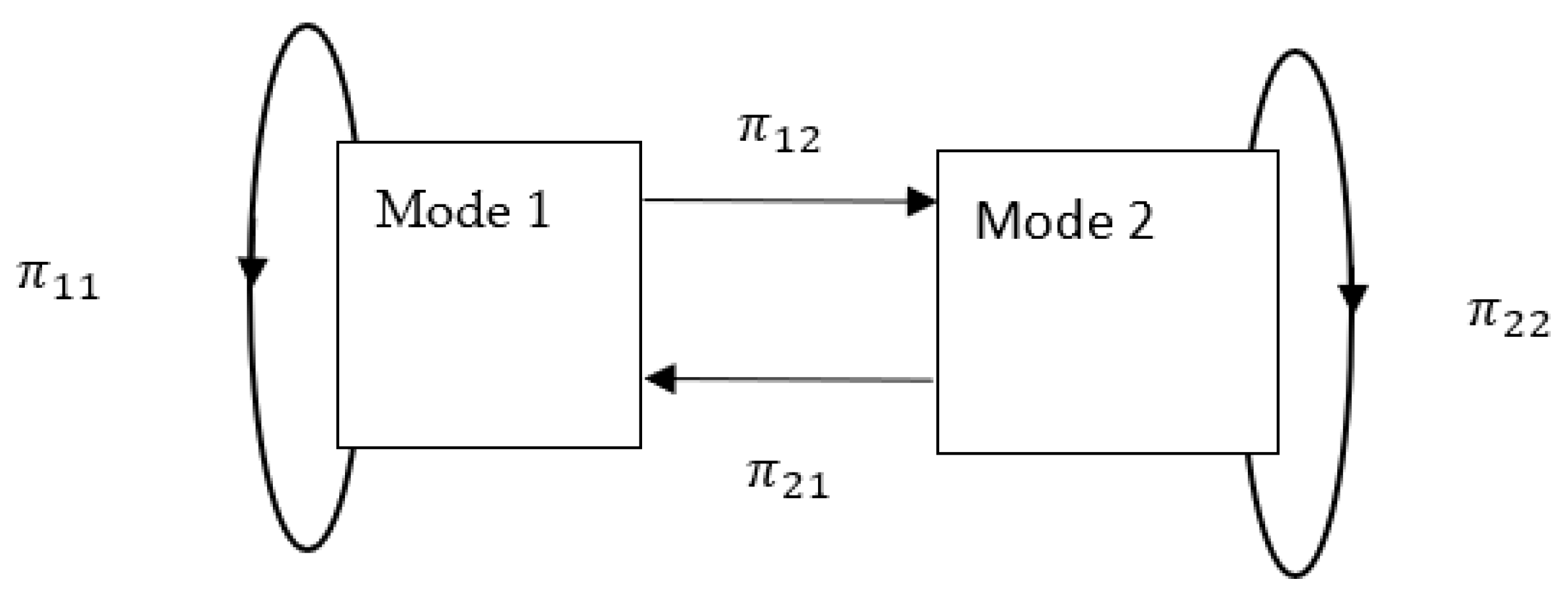
Figure 3.
State-space diagram of the highest and lowest reliability modes.
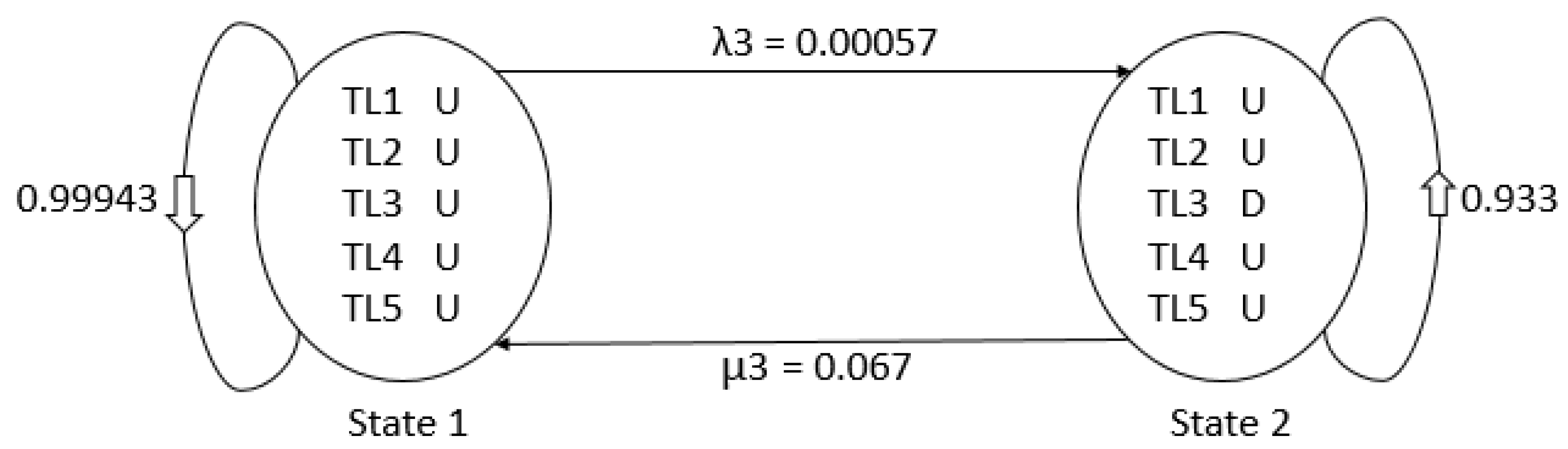
Figure 4.
External disturbance noise.
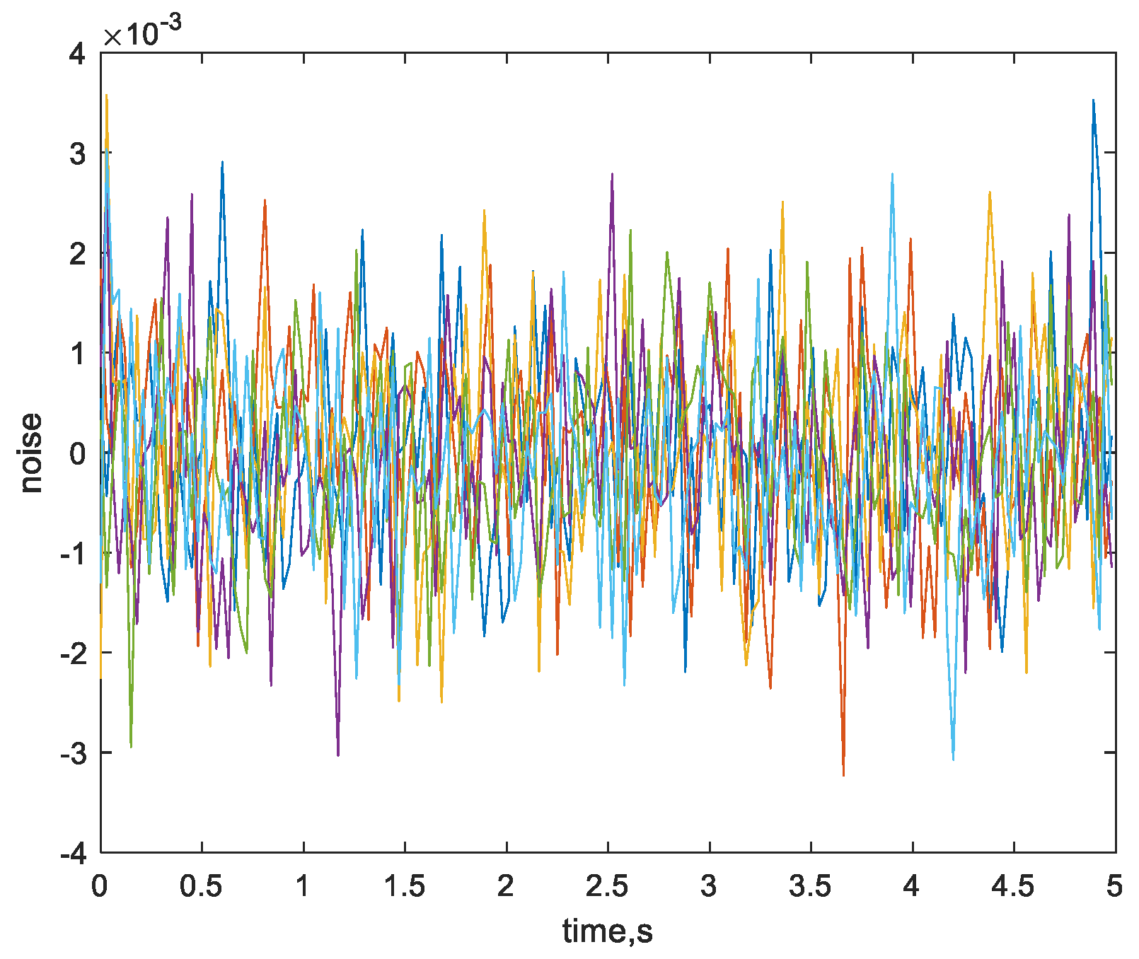
Figure 5.
Random mode switching; normal /contingency modes.
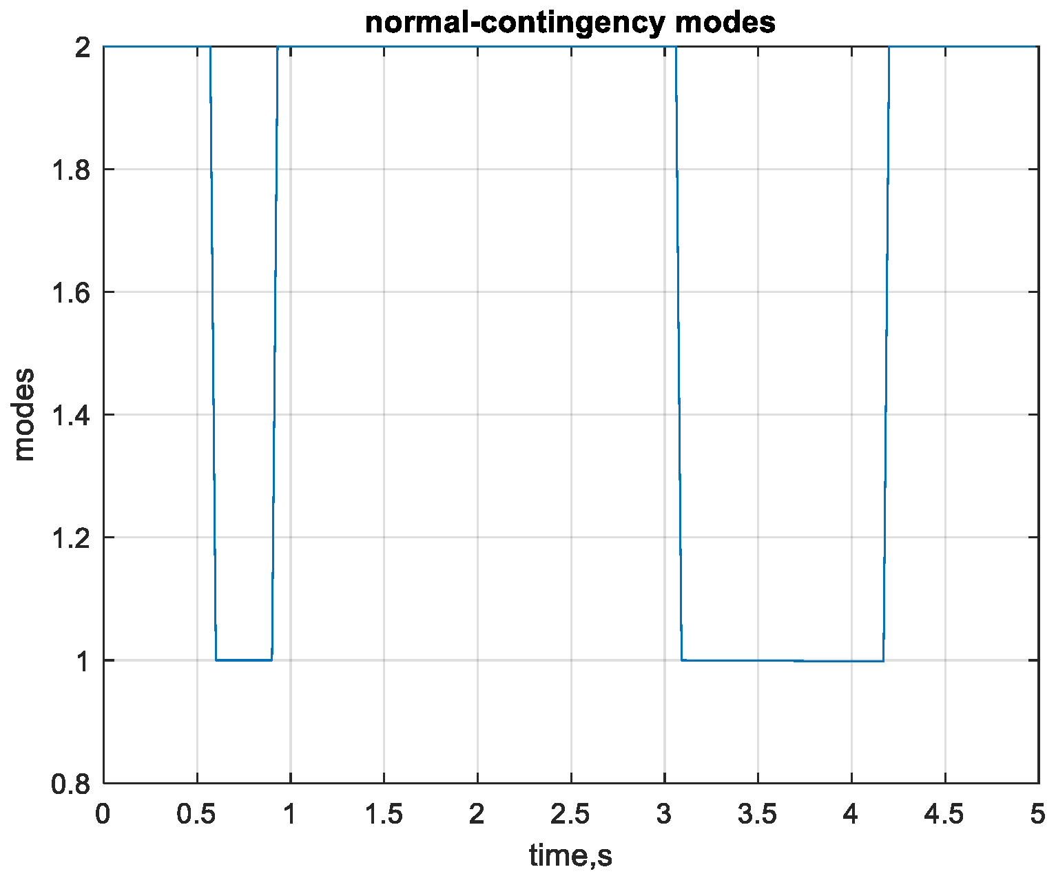
Figure 6.
Unstable response, without control. (a) Unstable response ( increases with time); (b) zoomed-in plot.
Figure 6.
Unstable response, without control. (a) Unstable response ( increases with time); (b) zoomed-in plot.

Figure 7.
Stable response, with control, nominal load.

Figure 8.
Control input, nominal load.
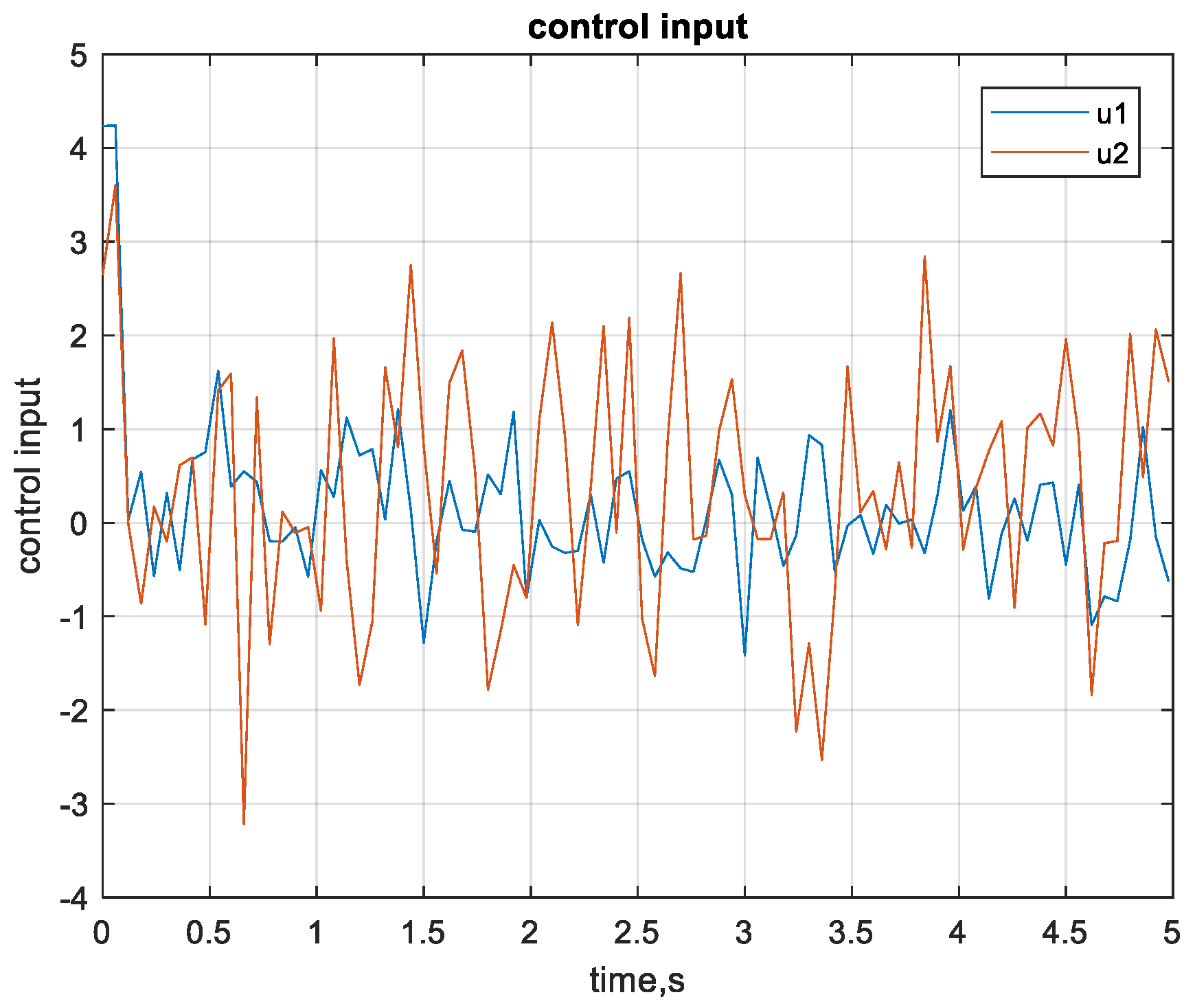
Figure 9.
Unstable response, with optimal control, nominal load.
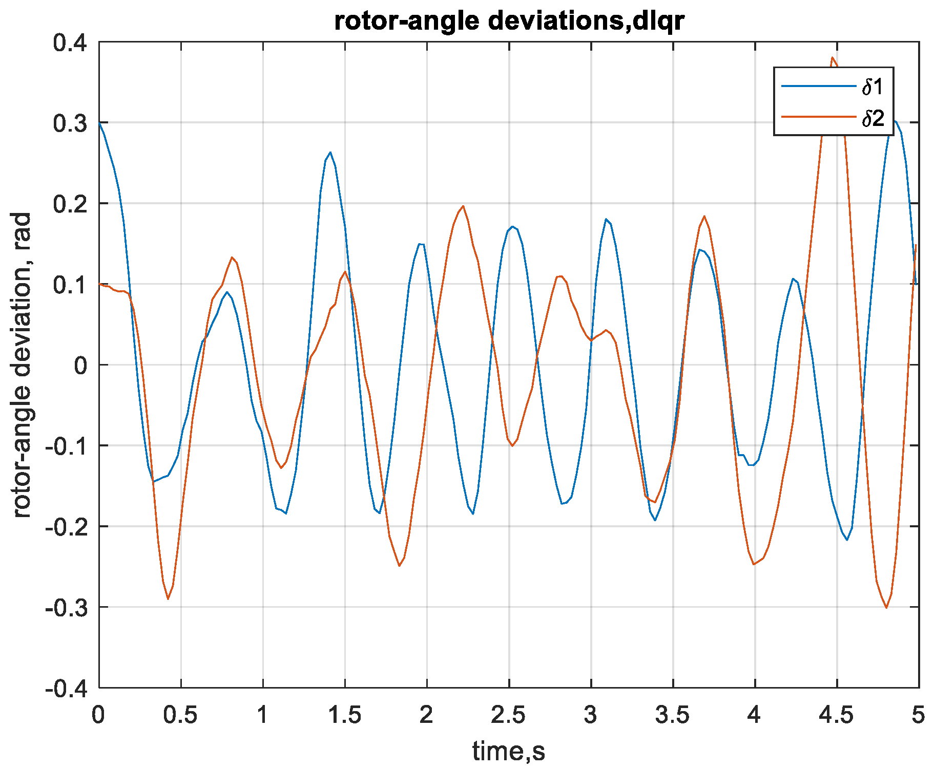
Figure 10.
Stable response, with control, 10% overload.

Figure 11.
Stable response, with control, 10% underload.


Table 1.
Nominal loading conditions and system data.
| Bus # | 1 | 2 | 3 | 4 | 5 | 6 |
|---|---|---|---|---|---|---|
| Gen-(MW) | - | 150 | 100 | - | - | - |
| Load-(MW) | - | - | - | 100 | 90 | 160 |
| Load-(MVAr) | - | - | - | 70 | 30 | 110 |
| 0.80 | 1.30 | 0.90 | - | - | - | |
| 0.80 | 1.30 | 0.90 | - | - | - | |
| 0.20 | 0.15 | 0.25 | - | - | - | |
| 9 | 5.80 | 6 | - | - | - | |
| H | 20 | 4 | 5 | - | - | - |
| AVR parameters | ||||||
| Ka | 25 | 25 | 25 | - | - | |
| Ta | 0.05 | 0.05 | 0.05 | - |
Table 2.
The electrical parameters of the power system.
| From Bus # | To Bus # | R(p.u) | X(p.u) | 0.5B(p.u) |
|---|---|---|---|---|
| 1 | 4 | 0.035 | 0.225 | 0.0065 |
| 1 | 5 | 0.025 | 0.105 | 0.0045 |
| 1 | 6 | 0.04 | 0.215 | 0.0055 |
| 2 | 4 | 0.0 | 0.035 | 0.0 |
| 3 | 5 | 0.0 | 0.042 | 0.0 |
| 4 | 6 | 0.028 | 0.125 | 0.0035 |
| 5 | 6 | 0.026 | 0.175 | 0.03 |
Table 3.
System reliability for different scenarios.
| All Lines Are Available | Line 1 Is on Outage | Line 2 Is on Outage | Line 3 Is on Outage | Line 4 Is on Outage | Line 5 Is on Outage |
|---|---|---|---|---|---|
| 0.983116 | 0.982902 | 0.982902 | 0.974569 | 0.982902 | 0.982902 |
Table 4.
Transition probability matrix.
| System Reliability Condition | State 1 | State 2 |
|---|---|---|
| Highest | 0.99943 | 0.00057 |
| Lowest | 0.067 | 0.933 |
Publisher’s Note: MDPI stays neutral with regard to jurisdictional claims in published maps and institutional affiliations. |
© 2022 by the authors. Licensee MDPI, Basel, Switzerland. This article is an open access article distributed under the terms and conditions of the Creative Commons Attribution (CC BY) license (https://creativecommons.org/licenses/by/4.0/).
Share and Cite
MDPI and ACS Style
Soliman, H.M.; El-Sheikhi, F.A.; Bayoumi, E.H.E.; De Santis, M. Ellipsoidal Design of Robust Stabilization for Markov Jump Power Systems under Normal and Contingency Conditions. Energies 2022, 15, 7249. https://doi.org/10.3390/en15197249
AMA Style
Soliman HM, El-Sheikhi FA, Bayoumi EHE, De Santis M. Ellipsoidal Design of Robust Stabilization for Markov Jump Power Systems under Normal and Contingency Conditions. Energies. 2022; 15(19):7249. https://doi.org/10.3390/en15197249
Chicago/Turabian StyleSoliman, Hisham M., Farag A. El-Sheikhi, Ehab H. E. Bayoumi, and Michele De Santis. 2022. "Ellipsoidal Design of Robust Stabilization for Markov Jump Power Systems under Normal and Contingency Conditions" Energies 15, no. 19: 7249. https://doi.org/10.3390/en15197249
Note that from the first issue of 2016, this journal uses article numbers instead of page numbers. See further details here.