
Study of the Harmonic Analysis and Energy Transmission Mechanism of the Frequency Conversion Transformer


1
College of Electrical and Information Engineering, Hunan University, Changsha 410012, China
2
TBEA Hengyang Transformer Co., Ltd., Hengyang 421000, China
3
Key Laboratory of Special Motors and High Voltage Electrical Appliances, Ministry of Education Shenyang, University of Technology, Shenyang 110178, China
*
Author to whom correspondence should be addressed.
Energies 2022, 15(2), 519; https://doi.org/10.3390/en15020519
Submission received: 29 November 2021
/
Revised: 6 January 2022
/
Accepted: 7 January 2022
/
Published: 12 January 2022
(This article belongs to the Topic Numerical Methods and Computer Simulations in Energy Analysis)
Abstract
:Since the transmission distance of submarine cable transmission is inversely proportional to the input frequency, to solve the problem of large losses in the transmission process of offshore wind power, this paper proposes a three-frequency transformer which enables the output of 50 Hz at the input of 50/3 Hz excitation. In this paper, the magnetic flux of a three-dimensional wound core transformer is analytically modeled, the existing condition of magnetic flux harmonics of a three-dimensional wound core transformer is analyzed, the distribution of harmonic content in magnetic flux is obtained, and the principle of realizing frequency conversion is expounded. Secondly, the finite element analysis of the frequency converter is carried out. Finally, a prototype of a frequency transformer is made and tested to verify the correctness of the proposed scheme.
1. Introduction
With people’s attention to the living environment, people begin to strengthen the development and utilization of some clean energy, such as solar energy, wind energy, and so on. Among them, offshore wind power has the advantages of no occupation of land, clean, small seasonal deviation, and so on. Each country begins to increase the investment in offshore wind power, but the transmission mode of offshore wind power is faced with the problems of large losses and high cost.
Professor Wang Xifan of Xi’an Jiaotong University proposed a low-frequency AC transmission mode. Frequency division transmission is a frequency division transmission method. In electric power transportation and distribution, changing the voltage frequency can achieve great economic benefits in transmission, transmitting electricity at lower frequencies and using electricity at higher frequencies. The key equipment of this technology is a frequency doubling transformer. Based on the three-phase low-frequency transmission method, Professor Wang has conducted a lot of research on its basic principle, feasibility, simulation and experimental platform construction [1,2,3]. The transmission distance of submarine cable is inversely proportional to the frequency used. If the transmission frequency is reduced to about 15 Hz, the economic and reasonable transmission distance of submarine cable can reach 300 km, which can completely solve the problem of offshore wind power transmission. Reducing the operating frequency of AC transmission lines can reduce the ground susceptance of the line and the reactive power required by the operation of the charge, to improve the active power transmission capacity of the transmission line.
On this basis, a kind of three-dimensional wound core transformer (three times frequency) is proposed. Compared with other types of same ration transformer, the three-dimensional wound core transformer with silicon steel sheet of the same material has many advantages, such as light weight, small volume, fewer core losses, and low noise. Therefore, more and more people began to study the three-dimensional wound core transformer. Alessandra Follo discussed three of them, which are discussed in his paper: the technological gap at the component level, controllability of DC collection systems, and compliance of all-DC OWPPs with current requirements for their connection to the onshore grids [4]. Pei Huang’s proposed method of studying the electric field distribution and analysis results are expected to contribute to the improvement of electric field distribution in transformers [5]. M. Rizwan Khan presents a digital simulation of a variable frequency transformer (VFT). The variable frequency transformer (VFT) is a device that produces desired voltage and frequency supply for constant and variable V/f control of an ac drive. The main part of the VFT is a rotary transformer with three-phase windings on both the stator and rotor. A controlled drive system is mechanically coupled with the VFT to control the speed of the rotor, therefore controlling the magnitude of rotor voltage and frequency [6]. Bharath Babu Ambati presents a detailed working principle of VFT technology and proposes a new hierarchical control strategy for establishing the VFT connection with two power systems to achieve bidirectional power transfer between them. Additionally, to restrict the grid fault propagation from one side of the VFT to the other side, a series dynamic braking-resistor-based fault ride-through scheme is proposed [7]. Zhou Pan proposes a flexible tuning device based on VFT to obtain different operating frequencies, so that the transmission line can meet the characteristics of half-wavelength AC transmission [8]. Vinod Khadkikar proposes a new VFT configuration (with an integrated partially rated series voltage compensation scheme and corresponding control) to achieve full control over reactive power flow. The proposed configuration can achieve the bidirectional and decoupled active and reactive power flow through VFT [9]. Traditional VFT requires a separate drive motor and winding asynchronous motor coaxial connection, unit shafting long, complex system structure, shaft vibration and tile amplitude value is high. To solve this problem, Guo Qifeng proposed a new structure variable frequency transformer integrating driving motor [10].
Based on the duality principle of three-dimensional wound core transformer, Pedram Elhaminia established the low-frequency model of three-dimensional wound core transformer, which is used to study steady-state and low-frequency transience [11]. Yaqian Yang presents a piecewise method for calculating the equivalent conductivity of a three-dimensional wound core transformer [12]. Based on the above method, the finite element model is established and the three-dimensional eddy current field is simulated. The effect of eddy current loss on wound core at different folding angles is studied. It is concluded that the magnetic flux density within the core is uneven and the third harmonic component is higher [13].
However, the current research on the magnetic flux in each frame of a three-dimensional wound core transformer is not perfect enough, and the realization of the frequency conversion function is not described from the perspective of magnetic flux of each frame. In this paper, based on magnetic circuit Kirchhoff’s Current Law and Kirchhoff’s Voltage Law, the constraint equation of the fixed solution of the magnetic flux in the frame is obtained, and the harmonic characteristics of the analytical solution are further analyzed. Finally, through the relationship between voltage and magnetic flux, SZ-RL-400/10 was used for finite element simulation, and a test platform was built to obtain voltage waveform, to verify the correctness of the proposed scheme.
2. Analytical Solutions of Framed Flux
Assume that the magnetic flux flowing through the three independent frames of the three-dimensional wound core transformer is , and , respectively, in which frame a and frame c constitute the A phase center column, frame b and frame a constitute the B phase center column, and frame b and frame c constitute the C phase center column, as shown in Figure 1 [14]. A, B and C are both windings and the locations where the phase flux converges.
It is known that the magnetic flux of phase A, phase B and phase C are , and , respectively. The constraint equation is obtained from the relationship between the magnetic flux of each frame and the phase magnetic flux as follows:
The determinant of the coefficients of the above equations is zero, and there is no unique solution to the equations, so another potential constraint equation needs to be introduced. Assume that the number of turns of the excitation coil is N, the reluctance of each frame is Rm, and the three-phase excitation current are , and , respectively. Since magnetic properties of iron core materials have obvious nonlinear characteristics, the reluctance Rm of each frame is a function of the magnetic field intensity of frame i as the independent variable. Based on magnetic circuit KVL, the constraint equation is created as follows.
According to (2), it can be obtained:
When the working points of magnetic circuits in each frame are located in the linear segment of magnetization curve, the reluctance of each frame is basically equal, then:
In the three-phase excitation system, the working point of the magnetic circuit in each frame is often different at any time [15,16,17]. At any time, the difference of three-phase reluctance increases with the increase in the magnetic circuit operating point. Then (4) is not equal to zero, let:
C is the zero-sequence component, , , n = 0, 1, 2, 3…, the zero-sequence component C increases with the increase of magnetic circuit operating point.
Combined with (1) and (5), the fixed solution equations are obtained as follows:
solution:
according to (1), the following can be obtained:
that is, there is no zero-sequence harmonic component in the phase flux, then let:
where: , n = 0, 1, 2, 3, …; , n = 0, 1, 2, 3…
Then substitute (9) into (7), and get:
where, (11) is a positive-sequence component of the positive-sequence harmonic; (12) is a negative-sequence component of the negative-sequence harmonic; (13) is a zero-sequence component of the zero-sequence harmonic.
3. Theoretical Analyses of Harmonic Components
The positive and negative sequence component harmonics in the split frame magnetic flux coming from the phase magnetic flux, namely the excitation voltage, so whether the excitation voltage can provide a high harmonic has a great influence on the waveform of the split frame magnetic flux [18]. The following focuses on analyzing the harmonic components of the core magnetic flux motivated by an ideal sine wave voltage source represented by an infinite system capacity voltage source and any waveform voltage source represented by a small system capacity voltage source.
3.1. Ideal Sine Wave Voltage Source
Under the excitation of an ideal sinusoidal voltage source, the magnetic flux of the split-core contains only the fundamental wave component and zero-sequence component harmonics. Suppose that the initial phase angle of fundamental wave flux is zero and the amplitude is one, then the flux waveform of the split-core can be described by the following equation.
where, i—harmonic number, , n = 0, 1, 2, 3,…, —the ith harmonic content, , —phase difference between the i th harmonic and the fundamental wave.
The waveform of and the harmonic component, the i th harmonic content rate ki and the i th harmonic are related to the phase difference between fundamental waves. Based on i = 3, ki = 0.2, , the influence of on waveform was studied, and the changing trend was shown in Figure 2a. It was concluded that the minimum waveform amplitude was obtained when , and the maximum waveform amplitude was obtained when , and was equal to (1 + ki). Based on i = 3, , ki ∈ [0, 0.6], the influence of ki on the waveform is studied, and the variation trend is shown in Figure 2b. It is concluded that waveform amplitude and ki are not monotonic and there is a minimum value. Based on , ki = 0.2, , the influence of i harmonic on the waveform is studied, and the variation trend is shown in Figure 2c. Wherein, the abscissa represents time and the ordinate represents flux magnitude. It is concluded that the higher the number of harmonics, the less significant the reduction in harmonic on the waveform amplitude.
Obviously, the amplitude of the waveform has a minimum value with respect to harmonic composition, content, and initial phase angle. The transformer core magnetic field in the passive region is a gradient field. Internally, the magnetic flux always chooses the path closure with the least reluctance, and externally, the magnetic flux always chooses the path closure with the least excitation magneto motive force. Therefore, the existence of zero-order harmonics is to obtain the minimum equivalent reluctance. The magnetization characteristics of common ferromagnetic materials are shown in Figure 3. With the further upward movement of the core working point, the magnetic conductivity rises at first and then sharply declines, as shown in Figure 4. If the magnetic circuit working point is located in the first half of Figure 4, the existence of the zero-sequence harmonic is to improve the amplitude of magnetic flux. When the working point of magnetic circuit is in the latter half, the existence of zero-order harmonics is to reduce the amplitude of magnetic flux.Since the magnetic circuit operating point of common electromagnetic devices is always located in the latter part, harmonic components can be obtained by finding the existence condition of the minimum value of Equation (11).
For the waveform with simple harmonic components, its minimum amplitude can be calculated based on the extreme value of a multivariate function under constraint conditions, and the solution of a constrained extreme value problem can be transformed into the solution of unconstrained extreme value problem, and it can also be solved based on the numerical analysis method of the enumeration method. Based on the extreme value calculation of multivariate function under constraint conditions, the minima problem under the action of single zero-order harmonics was analyzed. In order to reduce variables, could be set to construct the LaGrange function:
where , , . Figure out the stagnation point of Lagrange function , then, point is the extreme questionable point of function under the condition . To save space, the analytical solution is directly given as follows:
i = 3, 6, 9, 21… Substituted into (16), the calculation results are shown in Table 1. Obviously, as the number of harmonics increases, the number of suspicious extrema points increases, but there is less and less influence on the extremum, and the inclusion rate is reduced. The minimum value that can be obtained by waveform amplitude is of the fundamental wave.
The amplitude distribution of (14) is shown in Figure 5 when , , are drawn using enumeration method for numerical analysis based on MATLAB m language, and the numerical calculation results are consistent with the data in Table 1.
For waveforms with complex harmonic components, it is very difficult to obtain the minimum amplitude using an analytical method. A more convenient method is to adopt a numerical method. In order to intuitively display the influence of multicomponent harmonics on the amplitude, the extreme amplitude of the waveform of the third, ninth and third and fifteenth harmonics under different content rates is obtained, as shown in Figure 6. Under the action of multicomponent zero-sequence component harmonics, the minimum amplitude is still 2/3 of the fundamental wave.
3.2. Arbitrary Waveform Voltage Source
It is assumed that the voltage source can provide harmonics of positive and negative-sequence components, then the frame-divided flux waveform can contain harmonics of positive-sequence, negative-sequence, and zero-sequence components. The specific harmonic components make the resultant wave rectangular to obtain the minimum flux amplitude, as shown in Figure 7. The function is expressed in (17).
The Fourier series can be expanded as follows:
Then, the flux waveform is close to rectangular wave, the third harmonic content rate rises to 33.3%, and the amplitude value of the core flux decreases effectively. The amplitude of the synthesized waveform is 0.785 of the fundamental wave amplitudes.
4. Finite Element Simulation and Experimental Study
4.1. Finite Element Simulation
The filter coil FRa a, x, FRb b, y, FRc c, z, and the end of the three-filter coil is connected in turn. When c and x are disconnected (or connected in series to voltmeter), the circuit is in an open state, and the zero-sequence component harmonic flux can circulate freely in the core, then the opening voltage is zero-sequence harmonic voltage, as shown in Figure 8. When c and x are short-circuited (or connected in series to the ammeter), the loop is in a short-circuit state and the zero-sequence component harmonic flux cannot flow freely, then zero-sequence harmonic current will be generated in the loop, as shown in Figure 9.
The transformer parameters used in the paper are shown in Table 2.
The model was simulated by finite element software. Figure 10 shows the magnetic density distribution under different voltage excitation.
4.2. Test Platform
The test platform is built based on the core of a type SZ-RL-400/10 transformer. The excitation coil and synthetic flux induced voltage test coil are arranged on the three core pillars. The upper yoke of the three core frames is arranged with the framed flux induced voltage test coil and filter winding (FRa, FRb, and FRc), The test platform is shown in Figure 12.
4.3. Test Results
- Magnetic flux distribution of cores with and without zero-sequence paths;
When there is a zero-sequence flux path, each subframe flux contains abundant zero-sequence harmonic components. UA of column A and Ua of the frame a are shown in Figure 13a, and U3h of three-phase zero-sequence flux is shown in Figure 13b. When the zero-sequence flux closure path is not provided, each subframe flux does not contain the third harmonic, and its amplitude is of the phase flux. UA of column A and Ua of the induced flux voltage of frame a are shown in Figure 13c. In the absence of a zero-sequence path, the no-load loss, no-load current, and noise of the core increase significantly. The excitation voltage U, no-load loss P, no-load current I of the test data, and the induced voltage U3h or induced current I3h of the filter winding are summarized in Table 3.
- 2.
- Harmonic components of frame-separated flux with zero sequence path.
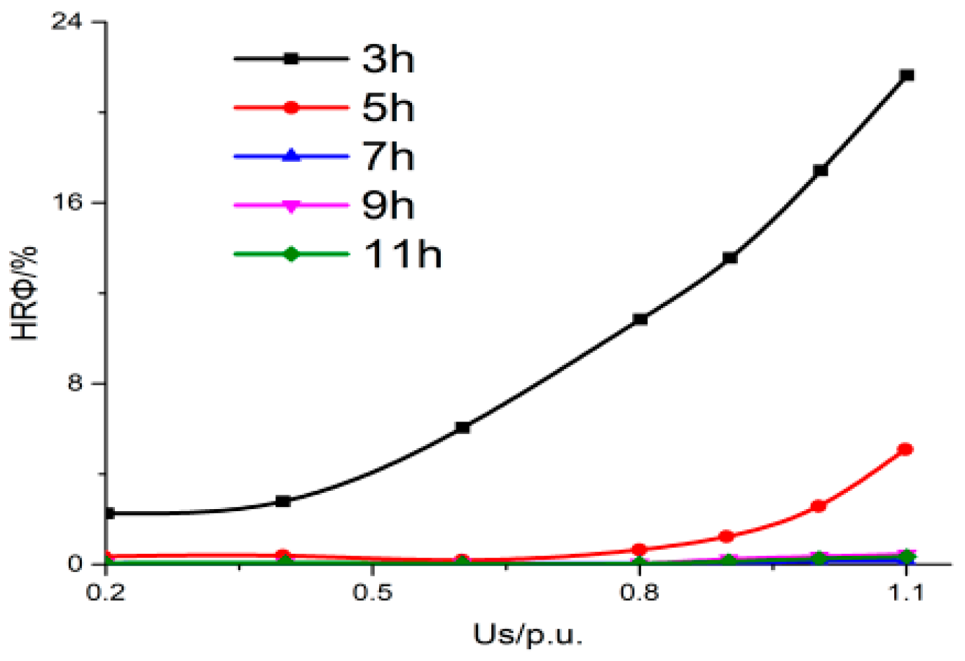
Figure 14 and Figure 15 show the distribution trends of the 3rd, 5th, 7th, 9th and 11th harmonic components in column A phase flux and frame a flux at 0.2~1.1 times of rated voltage. It can be seen from the figure that the frame flux contains zero-sequence harmonic components, mainly the third harmonic components, while the phase flux does not contain a zero-sequence harmonic component. With the rise of the core working point, the harmonic content rate increases continuously. The positive and negative-sequence harmonics of the phase flux are the same as those of the frame flux, that is, the positive and negative-sequence flux of the frame flux is 1/3 of the phase flux.
5. Conclusions
Frame-magnetic-flux of the positive-sequence, negative-sequence component is derived from the magnetic flux, and all of phase flux amplitude. The positive-sequence component of harmonic, frame flux lag phase flux 30, harmonic and negative-sequence component points frame flux 30° phase flux in advance. The zero sequence component is not included in the phase flux harmonics, and the points frame contained in the magnetic flux harmonic and the higher magnetic circuit working point of the zero sequence component contains three times more harmonic. In a certain sense, the frequency conversion function is realized. Then, the effectiveness of the proposed scheme is confirmed through the simulation of finite element simulation software and experimental verification.
Author Contributions
Writing—original draft preparation, Z.S.; Project administration, L.L.; Writing—review and editing, J.L., Z.L., H.L. and P.Z. All authors have read and agreed to the published version of the manuscript.
Funding
This research received no external funding.
Institutional Review Board Statement
Not applicable.
Acknowledgments
This research was supported by the Hunan youth talent project of China (2020RC3102).
Conflicts of Interest
The authors declare no conflict of interest.
References
- Wang, X. Frequency division Transmission System. China Electr. Power 1995, 1, 2–6. [Google Scholar]
- Teng, Y.; Ning, L.; Li, G.; Wang, X.; Lu, M. Mechanical and Electrical Transient Calculation Method and Transient Characteristic Analysis of Power System with Frequency Division Wind Power. Autom. Electr. Power Syst. 2015, 39, 43–50. [Google Scholar]
- Wang, X.; Zhang, X.; Ning, L.; Zhu, W.; Wang, X. Frequency transmission in the offshore wind power grid application prospects and challenges. Electr. Power Eng. 2017, 4, 15–19. [Google Scholar]
- Follo, A.; Saborío-Romano, O.; Tedeschi, E.; Cutululis, N.A. Challenges in All-DC Offshore Wind Power Plants. Energies 2021, 14, 6057. [Google Scholar] [CrossRef]
- Huang, P.; Mao, C.; Wang, D. Electric Field Simulations and Analysis for High Voltage High Power Medium Frequency Transformer. Energies 2017, 10, 371. [Google Scholar] [CrossRef] [Green Version]
- Khan, M.R.; Iqbal, A.; Ilahi, F. Digital Simulation of Variable Frequency Transformer. In Proceedings of the 2010 Joint International Conference on Power Electronics, Drives and Energy Systems & 2010 Power India, New Delhi, India, 20–23 December 2010; pp. 1–6. [Google Scholar]
- Ambati, B.B.; Kanjiya, P.; Khadkikar, V.; El Moursi, M.S.; Kirtley, J.L. A Hierarchical Control Strategy with Fault Ride-Through Capability for Variable Frequency Transformer. IEEE Trans. Energy Convers. 2014, 30, 132–141. [Google Scholar] [CrossRef] [Green Version]
- Zhou, P.; Ji, Y.; Dai, C.; Jing, P.; Zhao, C.; Wang, D. Application of frequency conversion transformer in half wavelength frequency conversion tuning. J. Electr. Power Syst. Autom. 2019, 31, 71–76. [Google Scholar]
- Ambati, B.B.; Khadkikar, V. Variable Frequency Transformer Configuration for Decoupled Active-Reactive Powers Transfer Control. IEEE Trans. Energy Convers. 2016, 31, 906–914. [Google Scholar] [CrossRef]
- Guo, Q. Research and Design of New Structure Variable Frequency Transformer. Master’s Thesis, China University of Mining and Technology, Xuzhou, China, 2014. [Google Scholar]
- Pedram, E.; Ehsan, H.; Ahmad, M.; Mehdi, V. Derivation of a Low-Frequency Model for a 3D Wound Core Transformer. In Proceedings of the 2017 Iranian Conference on Electrical Engineering, Tehran, Iran, 2–4 May 2017; pp. 1319–1323. [Google Scholar]
- Yang, Y.; Xu, J.; Zhou, J. A Segmented Paper Modeling Method of Open Transformer with Three-Dimensional Wound Core by Introducing Equivalent Conductivities. In Proceedings of the 2019 IEEE Transportation Electrification Conference and Expo, Asia-Pacific, Seogwipo, Korea, 8–10 May 2019; pp. 1–6. [Google Scholar]
- Loizos, G.; Kefalas, T.D.; Kladas, A.G.; Souflaris, A.T. Flux Distribution Analysis in Three-Phase Si-Fe Wound Transformer Cores. IEEE Trans. Magn. 2010, 46, 594–597. [Google Scholar] [CrossRef]
- Odawara, S.; Yamamoto, S. Iron Loss Evaluation of Reactor Core with Air Gaps by Magnetic Field Analysis Under High-Frequency Excitation. IEEE Trans. Magn. 2015, 51, 8402404. [Google Scholar] [CrossRef]
- Guo, X.; Song, D.; Long, L.; Xie, H.; Guan, T. Analysis of Basic Characteristics of S13 Three-Dimensional Wound-Core Transformer. Transformer 2012, 49, 27–37. [Google Scholar]
- Wu, Z.; Su, Z.; Zhang, X. Research of Operation Principle and Application Effect of Power Transformer Common Magnetic Shunt. Transformer 2018, 55, 24–31. [Google Scholar]
- Su, Z.; Zhang, C.; Tan, L. Application of Active Part Magnetic Shunt Circuit on Magnetic Leakage Prevention of Single Phase Transformer and Effectiveness Evaluation. Transformer 2015, 52, 24–28. [Google Scholar]
- Nezhivenko, S.; Bagheri, M.; Phung, T. Three-Dimensional Vibration Analysis of Single-Phase Transformer Winding under Inter-Disc Fault. In Proceedings of the 2017 International Symposium on Electrical Insulating Materials, Toyohashi, Japan, 11–15 September 2017; pp. 512–515. [Google Scholar]
Figure 1.
Schemes follow the same formatting.
Figure 2.
Flux waveform trends at different harmonics. (a) Based on i = 3, ki = 0.2, , the influence of on waveform. (b) Based on i = 3, , ki ∈ [0, 0.6], the influence of ki on the waveform. (c) Based on , ki = 0.2, , the influence of i harmonic on the waveform.
Figure 2.
Flux waveform trends at different harmonics. (a) Based on i = 3, ki = 0.2, , the influence of on waveform. (b) Based on i = 3, , ki ∈ [0, 0.6], the influence of ki on the waveform. (c) Based on , ki = 0.2, , the influence of i harmonic on the waveform.
Figure 3.
Magnetization characteristics.
Figure 4.
μ(H) curve.

Figure 5.
Distribution of waveform amplitude under single-component zero-order harmonics (a) 3rd harmonic; (b) 9th harmonic; (c) 15th harmonic; (d) 21st harmonic.
Figure 5.
Distribution of waveform amplitude under single-component zero-order harmonics (a) 3rd harmonic; (b) 9th harmonic; (c) 15th harmonic; (d) 21st harmonic.
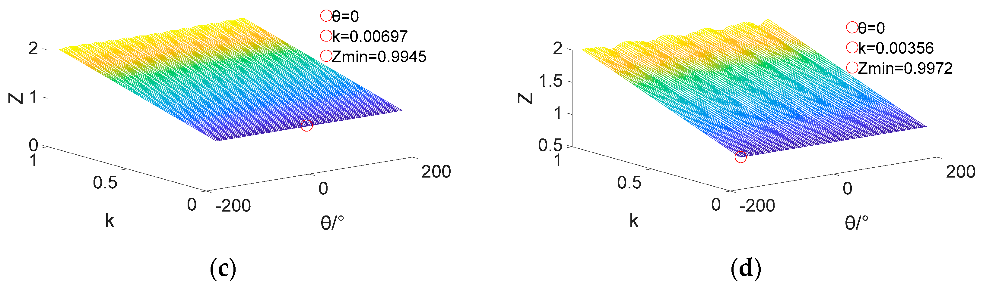
Figure 6.
Amplitude distribution of composite waves under multi-component zero-order harmonics (a) 3rd and 9th harmonics; (b) 3rd and 15th harmonics.
Figure 6.
Amplitude distribution of composite waves under multi-component zero-order harmonics (a) 3rd and 9th harmonics; (b) 3rd and 15th harmonics.
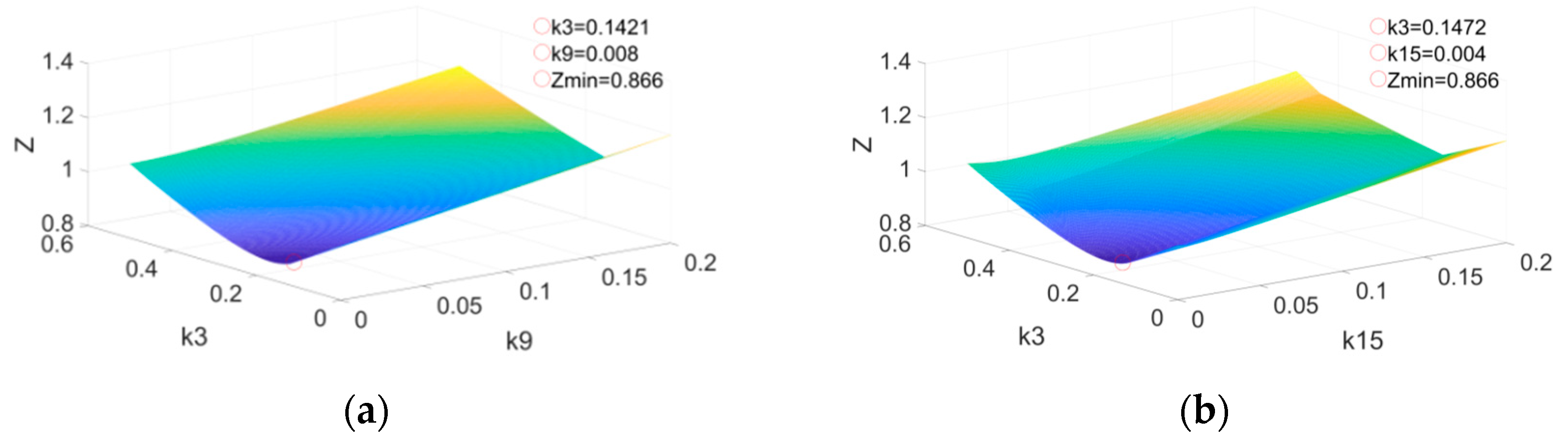
Figure 7.
Rectangular wave shape.
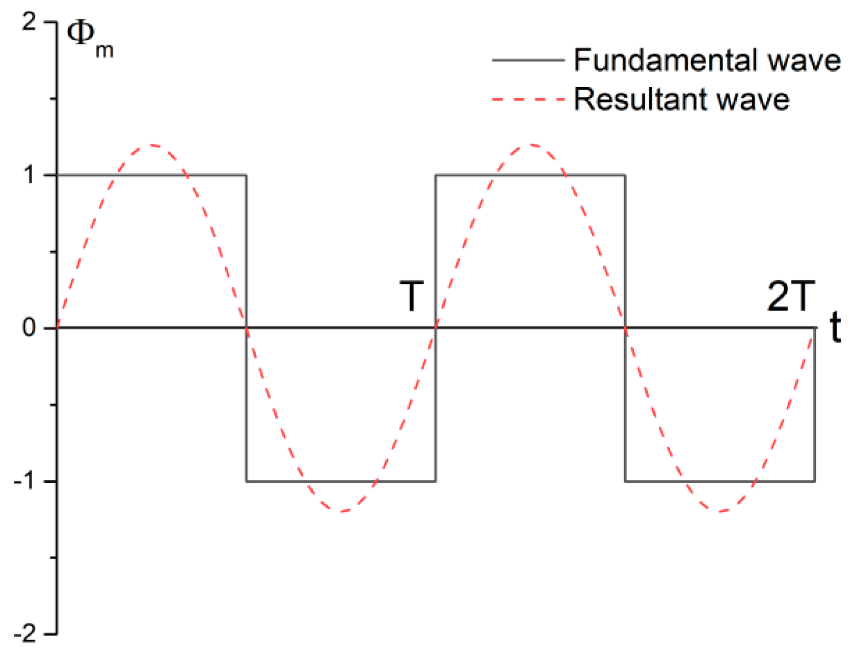
Figure 8.
Wiring diagram with zero sequence path.
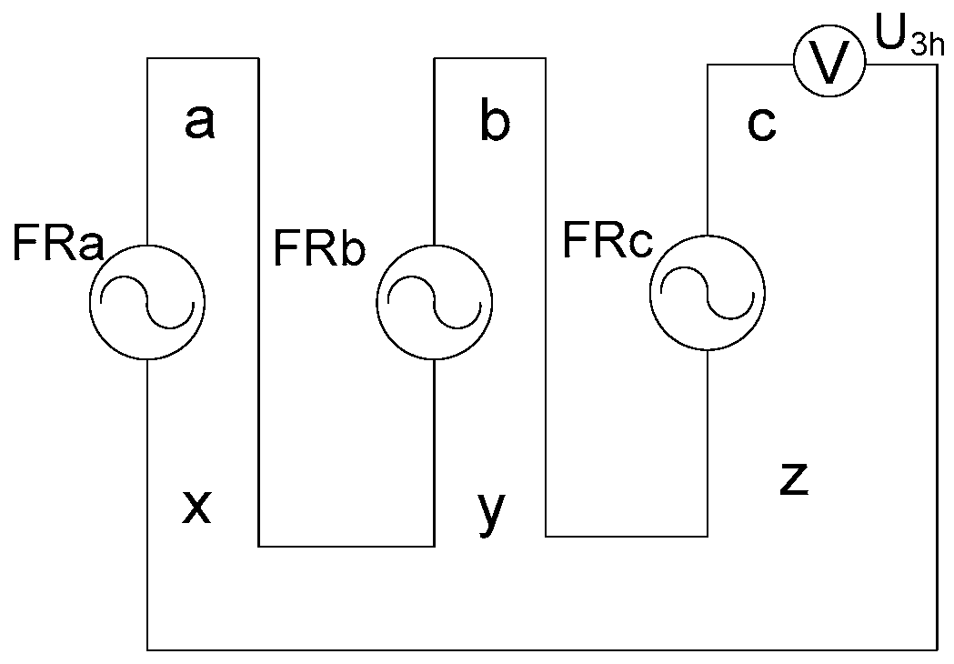
Figure 9.
Wiring diagram without zero sequence path.

Figure 10.
Magnetic density distribution under different voltage excitation (a) 0.9 times voltage excitation; (b) 1 times voltage excitation; (c) 1.05 times voltage excitation.
Figure 10.
Magnetic density distribution under different voltage excitation (a) 0.9 times voltage excitation; (b) 1 times voltage excitation; (c) 1.05 times voltage excitation.
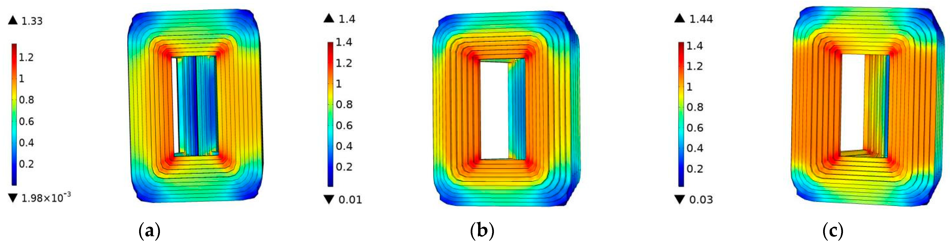
Figure 11.
Magnetic-flux-induced voltage simulation waveform. (a) The phase-flux-induced voltage UA of column A and the flux-induced voltage Ua of frame a with zero-sequence flux path; (b) the frequency spectrum diagram.
Figure 11.
Magnetic-flux-induced voltage simulation waveform. (a) The phase-flux-induced voltage UA of column A and the flux-induced voltage Ua of frame a with zero-sequence flux path; (b) the frequency spectrum diagram.
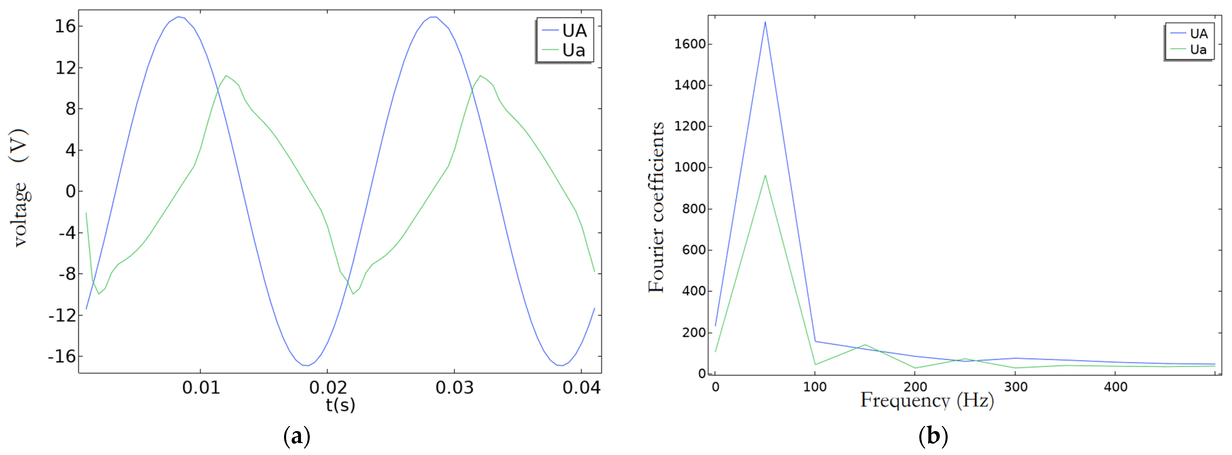
Figure 12.
Schemes follow the same formatting.
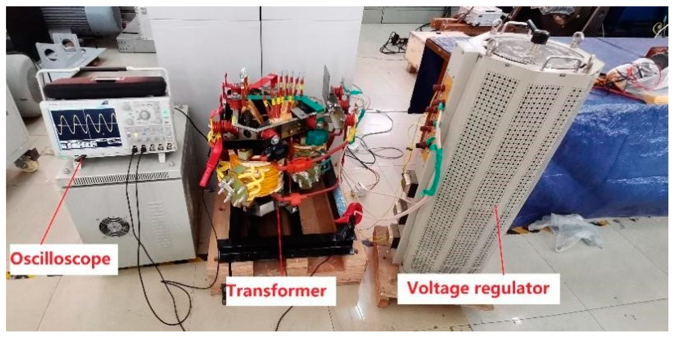
Figure 13.
Magnetic-flux-induced voltage test waveform.(a) When there is A zero-sequence flux path, phase flux induced voltage UA of column A and flux induced voltage Ua of the frame a. (b) When there is a zero-sequence flux path, phase flux induced voltage UA of column A and three phase zero sequence flux induced voltage U3h. (c) When the zero-sequence flux path is not provided, phase flux induced voltage UA of column A and flux induced voltage Ua of the frame a.
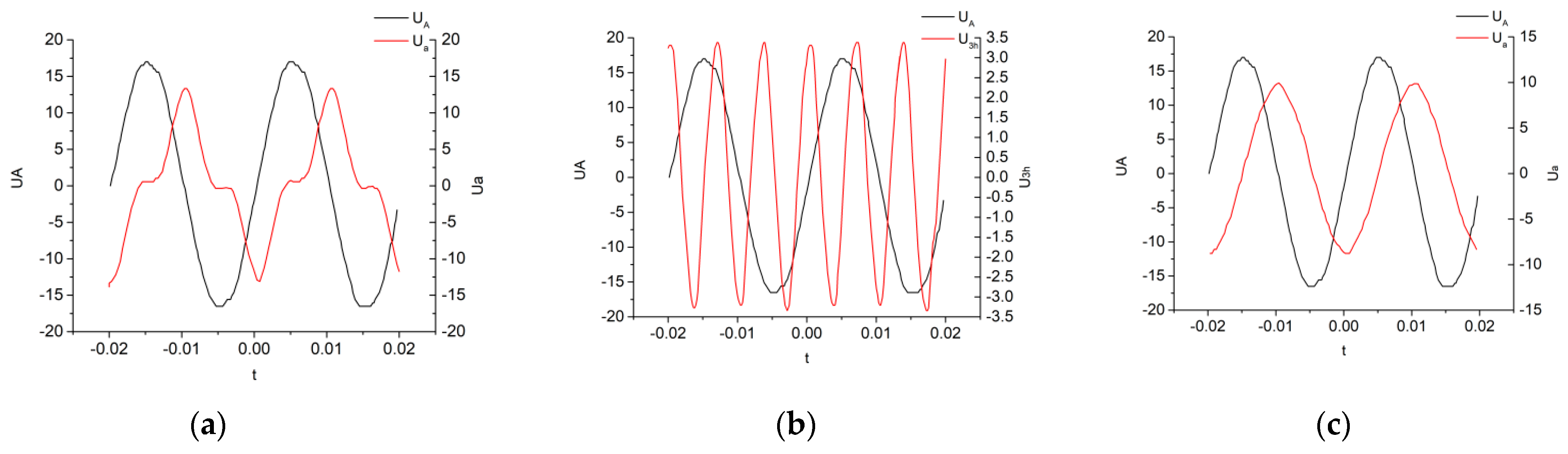
Figure 14.
Variation trend of phase flux harmonic content.
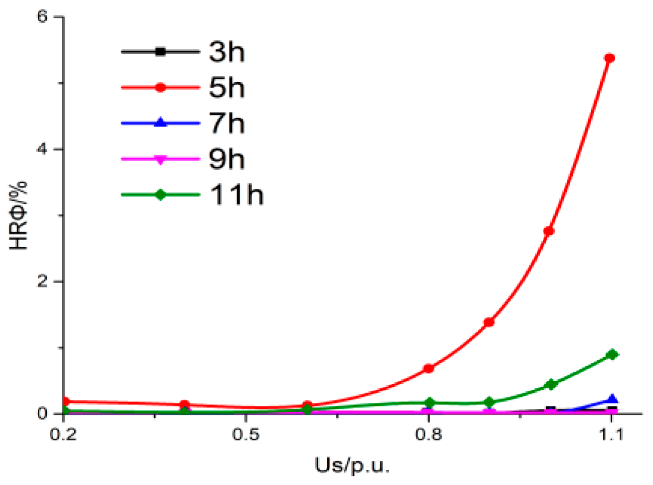
Figure 15.
Variation trend of frame flux harmonic content.

Table 1.
Results for different i values.
| i | 3 | 9 | 15 | 21 | 6n − 3 |
|---|---|---|---|---|---|
| ωt | 2π/3, 4π/3 | 5π/9, 13π/9 | 8π/15, 22π/15 | 11π/21, 31π/21 | kπ/(6n − 3) |
| ki | 16.667% | 1.93% | 0.697% | 0.356% | Cos(kπ/(6n − 3))/(6n − 3) |
| zmin | ±0.866 | ±0.9848 | ±0.9945 | ±0.9972 | ±Sin(kπ/(6n − 3)) |
Table 2.
Transformer parameters.
| Parameter | Value |
|---|---|
| Rated voltage | 400/10 |
| Rated current | 1.5/61 |
| Winding connection mode | Yd11 |
Table 3.
Experimental data with and without zero-sequence pathways.
| There Is a Zero-Sequence Flux Path | No Zero-Sequence Flux Path | ||||||||
|---|---|---|---|---|---|---|---|---|---|
| U/p.u. | U/V | I/A | P/kw | U3h/V | U/p.u. | U/V | I/A | P/kw | I3h/A |
| 0.9 | 206.79 | 1.13 | 0.325 | 2.56 | 0.9 | 207.22 | 1.5 | 0.373 | 2.8 |
| 1 | 230.99 | 1.53 | 0.433 | 3.42 | 1 | 231 | 7.5 | 0.633 | 21.3 |
| 1.05 | 241.78 | 2.18 | 0.514 | 3.98 | 1.05 | 243.65 | 21.96 | 1.091 | 71.8 |
Publisher’s Note: MDPI stays neutral with regard to jurisdictional claims in published maps and institutional affiliations. |
© 2022 by the authors. Licensee MDPI, Basel, Switzerland. This article is an open access article distributed under the terms and conditions of the Creative Commons Attribution (CC BY) license (https://creativecommons.org/licenses/by/4.0/).
Share and Cite
MDPI and ACS Style
Su, Z.; Luo, L.; Liu, J.; Li, Z.; Luo, H.; Zhao, P. Study of the Harmonic Analysis and Energy Transmission Mechanism of the Frequency Conversion Transformer. Energies 2022, 15, 519. https://doi.org/10.3390/en15020519
AMA Style
Su Z, Luo L, Liu J, Li Z, Luo H, Zhao P. Study of the Harmonic Analysis and Energy Transmission Mechanism of the Frequency Conversion Transformer. Energies. 2022; 15(2):519. https://doi.org/10.3390/en15020519
Chicago/Turabian StyleSu, Zhonghuan, Longfu Luo, Jun Liu, Zhongxiang Li, Hu Luo, and Peng Zhao. 2022. "Study of the Harmonic Analysis and Energy Transmission Mechanism of the Frequency Conversion Transformer" Energies 15, no. 2: 519. https://doi.org/10.3390/en15020519
Note that from the first issue of 2016, this journal uses article numbers instead of page numbers. See further details here.