Home Energy Management Strategy-Based Meta-Heuristic Optimization for Electrical Energy Cost Minimization Considering TOU Tariffs

Abstract

It is well documented that both solar photovoltaic (PV) systems and electric vehicles (EVs) positively impact the global environment. However, the integration of high PV resources into distribution networks creates new challenges because of the uncertainty of PV power generation. Additionally, high power consumption during many EV charging operations at a certain time of the day can be stressful for the distribution network. Stresses on the distribution network influence higher electricity tariffs, which negatively impact consumers. Therefore, a home energy management system is one of the solutions to control electricity consumption to reduce electrical energy costs. In this paper, a meta-heuristic-based optimization of a home energy management strategy is presented with the goal of electrical energy cost minimization for the consumer under the time-of-use (TOU) tariffs. The proposed strategy manages the operations of the plug-in electric vehicle (PEV) and the energy storage system (ESS) charging and discharging in a home. The meta-heuristic optimization, namely a genetic algorithm (GA), was applied to the home energy management strategy for minimizing the daily electrical energy cost for the consumer through optimal scheduling of ESS and PEV operations. To confirm the effectiveness of the proposed methodology, the load profile of a household in Udonthani, Thailand, and the TOU tariffs of the provincial electricity authority (PEA) of Thailand were applied in the simulation. The simulation results show that the proposed strategy with GA optimization provides the minimum daily or net electrical energy cost for the consumer. The daily electrical energy cost for the consumer is equal to 0.3847 USD when the methodology without GA optimization is used, whereas the electrical energy cost is equal to 0.3577 USD when the proposed methodology with GA optimization is used. Therefore, the proposed optimal home energy management strategy with GA optimization can decrease the daily electrical energy cost for the consumer up to 7.0185% compared to the electrical energy cost obtained from the methodology without GA optimization.

1. Introduction

Global warming is a reality and to control global warming, countries are implementing policies to reduce overall carbon dioxide emissions into the atmosphere. In this effort, emphasis has been given to clean energy sources such as solar photovoltaic (PV) and wind power for generating electricity instead of using fossil fuel. For transportation, electric vehicles (EVs) are promoted to replace combustion vehicles [1]. In Thailand, the government has a policy supporting electricity generation from renewable energy, such as electricity generation from solar PV rooftops [2], and promoting EV usage [3].

Increased usage of solar PV systems and EVs positively impact the global environment; however, a large number of PV systems and EVs connected to the distribution network can negatively impact the power system operation. For example, the intermittent power generation of PV systems can cause voltage variation in the distribution system. In addition, when the demand is less than the generation, power loss increases in the distribution system. The charging of EVs can also influence the distribution system in a lot of ways, for example, reliability and power quality issues because of line voltage drops due to a high charging demand. Moreover, an increase in the number of EVs can essentially affect the low voltage system with a high capability of energy consumption [4]. In reference [5], a case study on the effect of abundant solar PV installations in California, United States is presented. It was found that 80 to 90% of consumers charged their EVs during the peak period of 6:00 p.m. to 8:00 p.m. This situation increases the electrical energy cost for the consumer. Therefore, a home energy management strategy would help manage energy consumption in the household not only for lowering the electrical energy cost for the consumer but also for reducing the peak demand of the utility system.

1.1. Literature Review

Previous research works related to the rule-based home energy management strategy are proposed in this paragraph. In reference [6], the charging/discharging strategy of EVs for a home energy management system to obtain an economic benefit using a dynamic pricing scheme was proposed. In reference [7], a double layer supervision strategy for a flat power–load curve for residential consumers was proposed. In reference [8], a heuristic method was suggested to determine the most optimal charging/discharging of EVs in a time-of-day management system. This method simplified the structure using the input parameters, real-time prices, household demand, and EV parameters. This proposed algorithm can minimize the electrical energy cost for the consumer and the injected energy from the grid. In reference [9], a real-time decentralized demand-side management (RDCDSM) system was proposed to improve the real-time household load for estimating a day-ahead power production by the microgrid. Consumers should exploit the optimal energy management strategies for the charging/discharging of ESSs under their operational constraints. The RDCDSM can manage the uncertainties of the microgrid system through electrical power generation and purchase of day-ahead planning. Thus, the quality of power distribution to the consumers is increased. In reference [10], this work’s objective was the maximum utilization of solar PV systems for EV charging and to minimize the climate change problem related to CO₂ emissions. The energy generated by solar PV systems can be increased up to 13,792 kWh/year. Around 21% of the overall production can be applied to charge EVs, and the surplus energy can be injected into the federal grid. Furthermore, the proposed green transport methodology can decrease greenhouse gas emissions by 52,944 kg/year. In study [11], a stand-alone system for using the traditional household at the residential level in Bangladesh was proposed. The study aimed to determine the optimum size of a rooftop solar PV system that can support electrical appliance consumption at an affordable price. In reference [12], centralized and decentralized charging for EV schemes in residential buildings installing a solar PV system was proposed. The proposed methodologies were created to optimize the charging schedules of EVs for minimizing the overall load variance or flattening the net load profile. The minimization of the overall load variance indicates both an increase in the self-consumption of solar PV systems and a decrease in the peak residential loads. In reference [13], the methodology for minimizing the net cost of purchasing power from dissimilar energy sources, together with renewable energy generation from inside the microgrid, was proposed. In reference [14], an energy management system (EMS) to optimize power flows between solar PV systems, battery electric vehicles (BEVs), and the grid at the workspace was proposed. The objective was to minimize the charging cost of BEVs while decreasing power demand from the grid through increasing the sustainability of the BEVs and maximizing the self-consumption of the solar PV systems. The improved EMS had two main stages consisting of an autoregressive integrated moving average model to forecast the generated power of a solar PV system and a mixed-integer linear program (MILP) to appropriately manage power for minimizing the charging cost of BEVs. In reference [15], a two-stage energy management strategy of a solar PV system and an EV in a smart home for minimizing the electrical energy cost for the consumer and flattening the load profile was proposed. This strategy was classified into two stages, consisting of Stage A, which was determined as three operating modes following the unavailability of generated power from a solar PV system, and Stage B, which was determined as five operating modes following the availability of generated power from a solar PV system under a TOU rate.

The previous research works related to the rule-based home energy management strategy did not consider two significant issues, as follows:

(i).

They did not simultaneously consider the operations of three main components consisting of a solar PV system, an ESS, and a plug-in electric vehicle (PEV) in a household under TOU tariffs.

(ii).

They did not consider the energy consumption from a PEV journey or a vehicle to home (V2H) mode of PEV for supporting ESS operations.

In other words, the previous rule-based strategy did not consider a complex home energy management system.

The previous research works related to] optimal home energy management are presented in this paragraph. In reference [16], the works proposed the optimal power flow management strategy for a residential energy local network (RELN) consisting of a few smart homes, ESS, and PEV on the demand side, and a solar power plant and wind power plant on the supply side. Specifically, an appropriate and dynamic RELN power scheduling framework was established for minimizing the daily total operation cost while considering the error in the productivity forecast of renewable energy sources (RESs), user consumption, and the status of the energy storage system (ESS). As stated in reference [17], a home energy management system (HEMS) is demanding work that requires efficient domestic appliance schedules for optimizing energy consumption. In this work, they proposed a meta-heuristic method considering an HEMS using a combination of enhanced differential evolution (EDE) and a harmony search algorithm (HSA). Furthermore, they hybridized the HSA and EDE to optimize energy consumption. In reference [18], a practical HEMS model with renewable energy, ESS, and PEVs, with the sustainability of batteries and all-renewable energy in mind, was first created. Then, the correlation between the genetic algorithm (GA) and the multi-constrained integer programming was proposed. The objective was to minimize the purchasing power from the grid and to maximize renewable energy utilization. In reference [19], the methodology to manage HEMS models on a distribution system was proposed. Many heuristic strategies were reviewed and compared to motivate customers to adopt HEMS models. A case study was conducted using representative data. The results showed that the aging costs of transformers can be decreased through a prioritized magnitude by managing strategies and acceptance rates of HEMS models. In reference [4], an optimal EV charging schedule based on the energy arbitrage and the distribution system cost for the urban village environment was proposed. The proposed optimal charging scheme for EVs is focused on reducing the loss benefit because of energy arbitrage for the EV owner that reflects the penalty cost. Furthermore, power loss, peak demand, and transformer aging were combined in the evaluation in terms of the cost function for the distribution system. The authors of [20] presented a hierarchical deep reinforcement learning (DRL) scheme to schedule the energy consumption of appliances in smart homes and distributed energy resources (DERs) together with ESSs and EVs. A two-level DRL framework was presented. In the first level, the appliances in a house were scheduled based on the consumer preference and convenience level. In the second level, the schedules for the charging/discharging of EVs and ESSs were computed using the solution that was optimized from the first level with the characteristics of the consumer. Reference [21] proposed optimal building energy management considering solar PV systems and EVs to maximize solar PV utilization and optimize an EV charging schedule. In reference [22], energy management considering an energy price tag (EPT) of a smart house, including a solar PV system, an ESS, and an EV for minimizing the net electrical energy cost during the power demand, and the charging requirements of the ESS in the household was proposed. Additionally, energy management using a hierarchical DRL method was created for a smart home, including domestic appliances, a rooftop solar PV system, an EV, and an ESS to decrease electrical energy costs [23]. In reference [24], the optimal scheduling plan for household appliances and the charging/discharging procedure for ESSs and PEVs was presented. For this strategy, the coordination between an ESS and a PEV that can operate in the V2H mode during the peak demand time was proposed. This strategy can minimize the electrical energy cost for the consumer. Moreover, the charging power of an ESS or a PEV in this paper was not considered as an optimization problem.

The previous research works related to optimal home energy management systems did not consider three significant issues, as follows:

(i).

They did not consider the combination between the proposed rule-based home energy management strategy and the optimization mechanism.

(ii).

They did not consider the optimal charging processes of both an ESS and a PEV simultaneously in a household.

(iii).

They did not consider the charging power of an ESS or a PEV as an optimization problem.

The disregard for the three above-mentioned issues means the obtained ESS and PEV charging processes are not optimal. Therefore, the obtained electrical energy cost for a consumer is not the minimum as well.

1.2. The Contributions of This Research

In order to fulfill the above-mentioned gap of the previous research works, an optimal home energy management strategy that combines the rule-based method and the optimal-based method while considering the TOU tariffs is proposed. The main contributions of this research are summarized as follows:

• The proposed rule-based home energy management strategy considers two significant issues, as follows:

  (i).

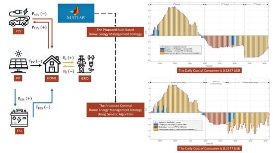
  The operations of all three main components in a household consisting of a solar PV system, an ESS, and a PEV, while considering TOU tariffs, are considered in this work.

  (ii).

  The energy consumption from a PEV journey and a PEV V2H mode for supporting ESS operations are taken into account.

• The proposed optimal home energy management strategy considers three significant issues, as follows:

  (i).

  The combination between the proposed rule-based home energy management strategy and the meta-heuristic optimization, namely a genetic algorithm (GA), is proposed. The objective function is the minimization of the electrical energy cost for the consumer.

  (ii).

  The optimal charging processes of both an ESS and a PEV in a household are considered.

  (iii).

  The charging powers of an ESS and a PEV are formulated as discrete functions, which are solved by using the GA.

The other sections of this paper are described as follows. Section 2 reports the proposed home energy management strategy. Section 3 explains the enhanced home energy management strategy combining GA optimization. The simulation results are shown and discussed in Section 4. Finally, the conclusion is presented in Section 5.

2. The Proposed Home Energy Management Strategy

The home energy management strategy to manage PEV and ESS charging/discharging schedules is proposed in this section. The charging/discharging algorithm for a PEV and an ESS was developed to apply in a household with a solar PV system, an ESS, and a PEV under the TOU tariffs in Thailand. The typical HEMS model is shown in Figure 1.

The surplus or insufficient power in each time slot when a PEV is not a load can be calculated using Equation (1) [24]. When a PEV is a load, the surplus or insufficient power can be calculated by Equation (2) [24].

$$P_1\left(t\right)=P_{\mathrm{PV}}\left(t\right)-P_{\mathrm{L}}\left(t\right)$$

(1)

$$P_1\left(t\right)=P_{\mathrm{PV}}\left(t\right)-P_{\mathrm{L}}\left(t\right)-P_{\mathrm{PEV}}\left(t\right)$$

(2)

When $P_1(t)$ in Equation (1) or (2) is greater than 0, it indicates that there is surplus power from the solar PV system installed in the household. Whereas when it is lower than 0, it indicates that the generated power from the solar PV system is insufficient to meet the power demand for the household. Furthermore, the charging/discharging states of ESS $\left(u_{\mathrm{ESS}}(t)\right)$ and PEV $\left(u_{\mathrm{PEV}}(t)\right)$ are used to decide whether the ESS and PEV will supply power to the household load, store surplus energy, or take no action.

To determine the charging/discharging state of the ESS for each time slot, $\left(u_{\mathrm{ESS}}(t)\right)$, which is a decision integer variable representing the chargeable and dischargeable power of the ESS of each time slot, is calculated using Equations (3) and (4) [24], respectively.

$$P_{\mathrm{ESS}}^{\mathrm{chable}}\left(t\right)=\frac{0.8C_{\mathrm{ESS}}^{\max }-C_{\mathrm{ESS}}\left(t-1\right)}{{\eta }_{\mathrm{ESS}}^{\mathrm{ch}}\Delta t}$$

(3)

$$P_{\mathrm{ESS}}^{\mathrm{dischable}}\left(t\right)=\frac{C_{\mathrm{ESS}}\left(t-1\right)-0.2C_{\mathrm{ESS}}^{\max }}{\Delta t}{\eta }_{\mathrm{ESS}}^{\mathrm{disch}}$$

(4)

According to Equation (3), when $P_{\mathrm{ESS}}^{\mathrm{chable}}(t)$ is more than 0, the charging/discharging state of the ESS $\left(u_{\mathrm{ESS}}(t)\right)$ is equal to 1, which indicates that the ESS can be charged. On the other hand, when $P_{\mathrm{ESS}}^{\mathrm{chable}}(t)$ is less than or equals 0, the ESS cannot be charged. Therefore, the ESS is not active when there is surplus power in the household. Similarly, in Equation (4), when $P_{\mathrm{ESS}}^{\mathrm{dischable}}(t)$ is more than 0, the charging/discharging state of the ESS $\left(u_{\mathrm{ESS}}(t)\right)$ is equal to 0, indicating the ESS can be discharged. On the other hand, when $P_{\mathrm{ESS}}^{\mathrm{dischable}}(t)$ is less than or equals 0, it indicates the ESS cannot be discharged. Therefore, the ESS is not active when there is insufficient power in the household.

The charging and discharging powers of ESS for each time slot are defined by Equations (5) and (6) [24], respectively.

$$P_{\mathrm{ESS}}^{\mathrm{ch}}\left(t\right)=\min \left(P_1\left(t\right),P_{\mathrm{ESS}}^{\mathrm{chable}}\left(t\right),P_{\mathrm{ESS}}^{\mathrm{chmax}}\right)$$

(5)

$$P_{\mathrm{ESS}}^{\mathrm{disch}}\left(t\right)=\max \left(P_1\left(t\right),P_{\mathrm{ESS}}^{\mathrm{dischable}}\left(t\right),P_{\mathrm{ESS}}^{\mathrm{dischmax}}\right)$$

(6)

The power and stored energy of the ESS for each time slot can be calculated using Equations (7) and (8) [6], respectively.

$$P_{\mathrm{ESS}}\left(t\right)=P_{\mathrm{ESS}}^{\mathrm{ch}}\left(t\right)u_{\mathrm{ESS}}\left(t\right)+P_{\mathrm{ESS}}^{\mathrm{disch}}\left(t\right)\left(1-u_{\mathrm{ESS}}\left(t\right)\right)$$

(7)

$$C_{\mathrm{ESS}}\left(t\right)=C_{\mathrm{ESS}}\left(t-1\right)+P_{\mathrm{ESS}}^{\mathrm{ch}}\left(t\right)u_{\mathrm{ESS}}\left(t\right)\Delta t{\eta }_{\mathrm{ESS}}^{\mathrm{ch}}+\frac{P_{\mathrm{ESS}}^{\mathrm{disch}}\left(t\right)\left(1-u_{\mathrm{ESS}}\left(t\right)\right)\Delta t}{{\eta }_{\mathrm{ESS}}^{\mathrm{disch}}}$$

(8)

To determine the charging/discharging state of the PEV for each time slot, $\left(u_{\mathrm{PEV}}(t)\right)$ which is a decision integer variable representing the chargeable or dischargeable power of the PEV for each time slot, can be calculated using Equations (9) and (10) [24], respectively.

$$P_{\mathrm{PEV}}^{\mathrm{chable}}\left(t\right)=\frac{0.8C_{\mathrm{PEV}}^{\max }-C_{\mathrm{PEV}}\left(t-1\right)}{{\eta }_{\mathrm{PEV}}^{\mathrm{ch}}\Delta t}$$

(9)

$$P_{\mathrm{PEV}}^{\mathrm{dischable}}\left(t\right)=\frac{C_{\mathrm{PEV}}\left(t-1\right)-0.3C_{\mathrm{PEV}}^{\max }}{\Delta t}{\eta }_{\mathrm{PEV}}^{\mathrm{disch}}$$

(10)

When $P_{\mathrm{PEV}}^{\mathrm{chable}}(t)$ in Equation (9) is more than 0, the charging/discharging state of PEV $\left(u_{\mathrm{PEV}}(t)\right)$ is equal to 1 and indicates that the PEV can be charged. On the other hand, when $P_{\mathrm{PEV}}^{\mathrm{chable}}(t)$ is less than or equals 0, it indicates that the PEV cannot be charged. Therefore, the PEV is not active when there is surplus power in the household or when it is operating as a load. Similarly, when $P_{\mathrm{PEV}}^{\mathrm{dischable}}(t)$ is more than 0, the charging/discharging state of PEV $\left(u_{\mathrm{PEV}}(t)\right)$ is equal to 0, which indicates that the PEV can be discharged. On the other hand, when $P_{\mathrm{PEV}}^{\mathrm{dischable}}(t)$ is less than or equals 0, it indicates that the PEV cannot be discharged. Therefore, the PEV is not active when there is insufficient power in the household.

When the PEV is operated in V2H mode in the second period, the charging and discharging powers of the PEV for each time slot are defined by Equations (11) and (12) [24], respectively.

$$P_{\mathrm{PEV}}^{\mathrm{ch}}\left(t\right)=\min \left(P_1\left(t\right),P_{\mathrm{PEV}}^{\mathrm{chable}}\left(t\right),P_{\mathrm{PEV}}^{\mathrm{chmax}}\right)$$

(11)

$$P_{\mathrm{PEV}}^{\mathrm{disch}}\left(t\right)=\max \left(P_1\left(t\right),P_{\mathrm{PEV}}^{\mathrm{dischable}}\left(t\right),P_{\mathrm{PEV}}^{\mathrm{dischmax}}\right)$$

(12)

When the PEV is operating as a load in the third period, the PEV is continuously charged until the stored energy of the PEV is more than 80% of its maximum capacity at the time slot before the PEV leaves the household. The PEV is charged using Equations (13)–(15) [24], respectively.

$$P_{\mathrm{D}}\left(t\right)=P_{\mathrm{G}}^{\max }-P_{\mathrm{L}}\left(t\right)$$

(13)

$$P_{\mathrm{PEV}}^{\mathrm{chable}}\left(t\right)=\frac{C_{\mathrm{PEV}}^{\max }-C_{\mathrm{PEV}}\left(t\right)}{\Delta t}{\eta }_{\mathrm{ESS}}^{\mathrm{ch}}$$

(14)

$$P_{\mathrm{PEV}}^{\mathrm{ch}}\left(t\right)=\min \left(P_{\mathrm{D}}\left(t\right),P_{\mathrm{PEV}}^{\mathrm{chable}}\left(t\right),P_{\mathrm{PEV}}^{\mathrm{chmax}}\right)$$

(15)

The power and stored energy of the PEV for each time slot can be calculated using Equations (16) and (17) [24], respectively.

$$P_{\mathrm{PEV}}\left(t\right)=P_{\mathrm{PEV}}^{\mathrm{ch}}\left(t\right)u_{\mathrm{PEV}}\left(t\right)+P_{\mathrm{PEV}}^{\mathrm{disch}}\left(t\right)\left(1-u_{\mathrm{PEV}}\left(t\right)\right)$$

(16)

$$C_{\mathrm{PEV}}\left(t\right)=C_{\mathrm{PEV}}\left(t-1\right)+P_{\mathrm{PEV}}^{\mathrm{ch}}\left(t\right)u_{\mathrm{PEV}}\left(t\right)\Delta t{\eta }_{\mathrm{PEV}}^{\mathrm{ch}}+\frac{P_{\mathrm{PEV}}^{\mathrm{disch}}\left(t\right)\left(1-u_{\mathrm{PEV}}\left(t\right)\right)\Delta t}{{\eta }_{\mathrm{PEV}}^{\mathrm{disch}}}$$

(17)

The power between the household and grid for each time slot when the PEV is not parked and when it is parked at the household can be defined using Equations (18) and (19) [24], respectively.

$$P_{\mathrm{G}}\left(t\right)=P_{\mathrm{PV}}\left(t\right)-P_{\mathrm{L}}\left(t\right)-P_{\mathrm{ESS}}\left(t\right)$$

(18)

$$P_{\mathrm{G}}\left(t\right)=P_{\mathrm{PV}}\left(t\right)-P_{\mathrm{L}}\left(t\right)-P_{\mathrm{ESS}}\left(t\right)-P_{\mathrm{PEV}}\left(t\right)$$

(19)

When $P_{\mathrm{G}}(t)$ is more than 0, it indicates that there is still surplus power from the solar PV system in the household and the power is being injected into the utility grid, thus lowering the electrical energy cost for the consumer. On the other hand, when $P_{\mathrm{G}}(t)$ is less than 0, it can be said that the power from the solar PV system is insufficient for the household load; therefore, power is drawn from the utility grid, thus increasing the electric energy cost for the consumer. Finally, the electrical energy cost for the consumer for each time slot can be calculated using Equation (20).

$$cost\left(P_{\mathrm{G}}\left(t\right)\right)=\{\begin{array}{c}{P}_{\mathrm{G}}\left(t\right)\cdot TOU\left(t\right)\cdot \Delta t\\ P_{\mathrm{G}}\left(t\right)\cdot FiT\cdot \Delta t\end{array}\begin{array}{c};P_{\mathrm{G}}\left(t\right)<0\\ ;P_{\mathrm{G}}\left(t\right)>0\end{array}$$

(20)

Typically, the home energy management strategy in a day is divided into three periods based on the PEV usage. The steps of the proposed home energy management strategy are presented in Figure 2 and are described in Section 2.1.

2.1. Energy Management Strategy in the First Period

The first period represents the time interval starting at 07:00 a.m., when the PEV leaves the house, to when it returns home at 06:00 p.m. The energy management strategy for each time slot during the first period is described below.

(1)

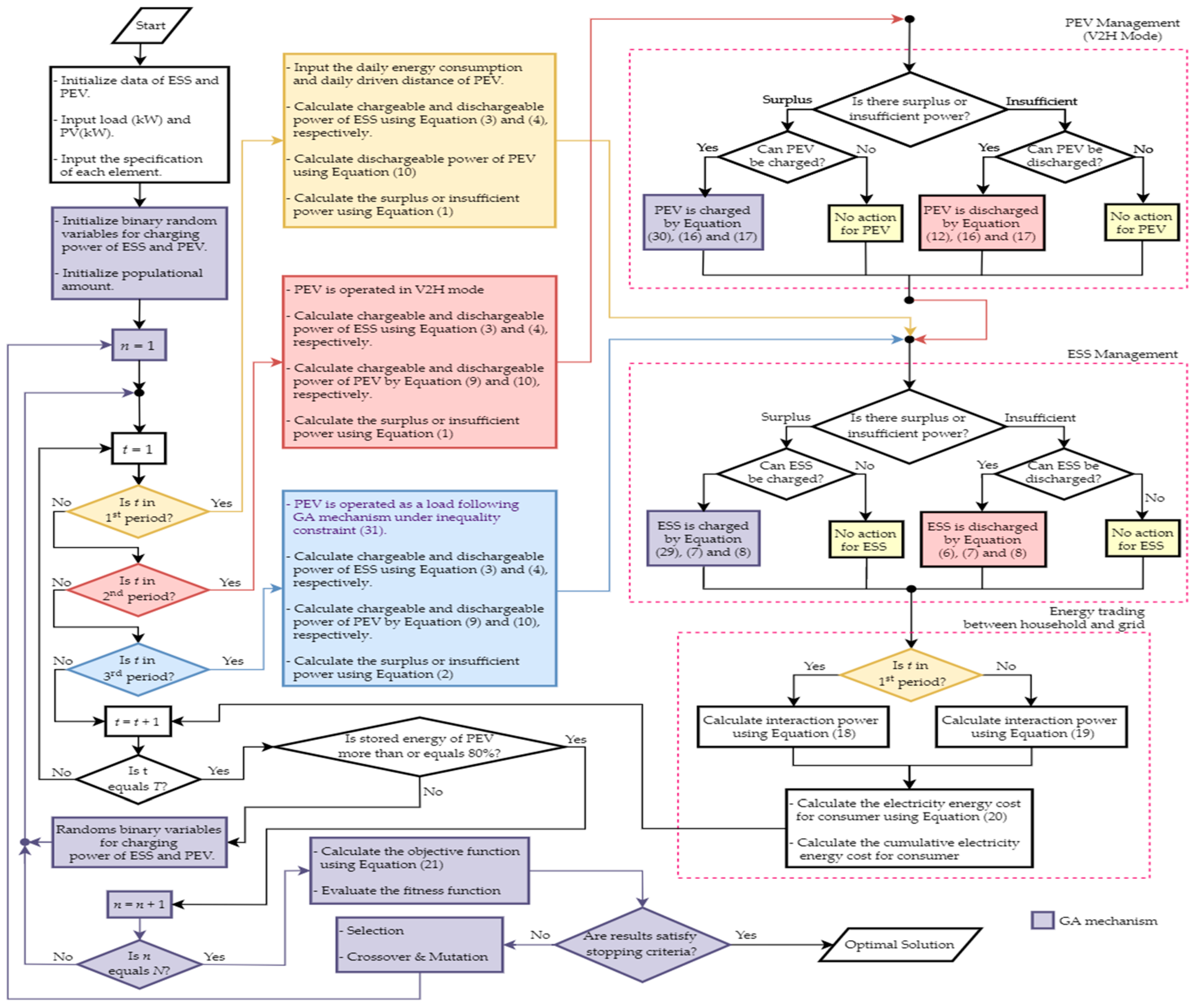
First, the data of the ESS, PEV, household load, and PV system are the initial inputs for each time slot. Additional inputs include the daily energy consumption of the PEV (kWh/km), the daily driven distance (km) of PEV during the day, and so forth. Moreover, the discharging state of the PEV $\left(u_{\mathrm{PEV}}(t)\right)$ for the period from 10:15 p.m. to 06:45 a.m. is initialized as 0, which continuously changes following the home energy management mechanism, as shown in Figure 2.

(2)

The chargeable and dischargeable powers of the ESS are calculated using Equations (3) and (4), respectively. The dischargeable power of the PEV is calculated using Equation (10). Then, the surplus or insufficient power is calculated using Equation (1).

(3)

In this step, if there is surplus power in the household and the charging/discharging state of ESS $\left(u_{\mathrm{ESS}}(t)\right)$ is indicated to be 1, the ESS will be charged following Equation (5). If there is insufficient power in the household and the charging/discharging state of ESS $\left(u_{\mathrm{ESS}}(t)\right)$ is indicated to be 0, the ESS will be discharged following Equation (6). Lastly, the power and stored energy of the ESS are calculated using Equations (7) and (8), respectively.

(4)

Finally, $P_{\mathrm{G}}(t)$ is calculated using Equation (18). Then, the electrical energy cost for the consumer is calculated using Equation (20).

2.2. Energy Management Strategy in the Second Period

The second period starts at 06:00 p.m., when the PEV returns home. The finish time of the second period is initialized as 06:45 a.m., with the conditions having continuously changed as per the home energy management mechanism, as shown in Figure 2. Overall conditions change because the PEV operates in V2H mode to support the ESS operation and minimize the purchasing power from the grid during the peak time interval. The proposed energy management strategy for each time slot during this period is presented in Figure 2 and is described below.

(1)

Firstly, the ESS and PEV data are initialized with the load demand, and the PV power for each time slot are the input variables.

(2)

The chargeable and dischargeable powers of the ESS are calculated using Equations (3) and (4), respectively. The chargeable and dischargeable powers of the PEV are calculated using Equations (9) and (10), respectively. Then, the surplus or insufficient power is calculated using Equation (1).

(3)

In this step, if there is surplus power in the household and the PEV can be charged, the PEV will be charged following Equation (11). If there is insufficient power in the household and the PEV can be discharged, the PEV will be discharged following Equation (12). In addition, the power and stored energy of the PEV will be calculated using Equations (13) and (14), respectively.

(4)

If there is still surplus power in the household and the charging/discharging state of ESS $\left(u_{\mathrm{ESS}}(t)\right)$ is indicated to be 1, the ESS will be charged following Equation (5). If there is insufficient power in the household and the charging/discharging state of ESS $\left(u_{\mathrm{ESS}}(t)\right)$ is indicated to be 0, the ESS will be discharged following Equation (6). Lastly, the power and stored energy of the ESS will be computed for each time slot using Equations (7) and (8), respectively.

(5)

Finally, $P_{\mathrm{G}}(t)$ is calculated using Equation (19). Then, the electrical energy cost for the consumer is calculated using Equation (20).

2.3. Energy Management Strategy in the Third Period

The third period is the interval time after the second period until 07:00 a.m. In this section, the PEV operates as a load. The home energy management strategy for each time slot of the third period is described below:

(1)

Firstly, the ESS and PEV data are initialized. Then, the load demand and the PV power of each time slot and the specification of each element are imported to be input variables. In this period, the PEV is operated as a load following the algorithm in Figure 2.

(2)

The chargeable and dischargeable powers of the ESS are computed using Equations (3) and (4), respectively. The dischargeable power of the PEV is computed using Equation (10). The surplus or insufficient power is calculated using Equation (2).

(3)

When the charging/discharging state of PEV $\left(u_{\mathrm{PEV}}(t)\right)$ is equal to 1, the PEV is operated as a load, following Equations (13)–(15), respectively.

(4)

In this step, if there is surplus power in the household and the ESS can be charged, the ESS will be charged following Equation (5). If there is insufficient power in the household and the ESS can be discharged, the ESS will be discharged following Equation (6). In addition, the power and stored energy of the ESS will be calculated using Equations (7) and (8), respectively.

(5)

Finally, $P_{\mathrm{G}}(t)$ is calculated using Equation (19). Then, the electrical energy cost for the consumer is calculated using Equation (20).

It should be noted that when the charging state of PEV $\left(u_{\mathrm{PEV}}(t)\right)$ is 1, it indicates that the PEV can be charged. This action starts from the last time slot and continuously reverses to the previous time slot until the stored energy of the PEV is more than or equal to 80% of its maximum capacity at the slot before the PEV leaves the household. If the above-mentioned is true, the home energy management in a day is complete.

3. The Proposed Home Energy Management Strategy with Genetic Algorithm

Previous research works have not considered the charging equations for both the ESS and PEV as a problem for optimization, as shown in Equations (5) and (11). Moreover, in order to minimize the total cost for a consumer, the charging powers of both the ESS and PEV, as represented in Equations (5) and (11), respectively, have to be minimized. Hence, these two equations were formulated as the discrete function in this work. The GA, which is suitable for optimizing the discrete function effectively, was chosen. Any values between zero and these two equations’ values were randomized using the “rand” function in the MATLAB program.

The objective of the proposed optimal home energy management strategy combined with GA optimization is to minimize the overall electrical energy cost for the consumer. The objective and constraint functions are defined as follows.

3.1. Objective Function

The objective function is to minimize the electrical energy cost for the consumer, as shown in Equation (21) below.

$$\min \left[cos{t}_{\mathrm{daily}}\right]={\displaystyle \sum _{t=1}^{T}cost\left(P_{\mathrm{G}}\left(t\right)\right)}$$

(21)

3.2. Constraints

The charging/discharging powers for the ESS and PEV can be improved following the surplus/insufficient power from the solar PV system for each time slot. However, they have to be adjusted between the upper and lower specification limits to protect the overloading operation. Thus, the charging powers of the ESS and PEV for each time slot have to be limited following the two inequality constraint functions in Equations (22) and (23) [24], respectively.

$$0\le P_{\mathrm{ESS}}^{\mathrm{ch}}\left(t\right){\eta }_{\mathrm{ESS}}^{\mathrm{ch}}\le P_{\mathrm{ESS}}^{\mathrm{chmax}}\left(t\right)$$

(22)

$$0\le P_{\mathrm{PEV}}^{\mathrm{ch}}\left(t\right){\eta }_{\mathrm{PEV}}^{\mathrm{ch}}\le P_{\mathrm{PEV}}^{\mathrm{chmax}}\left(t\right)$$

(23)

In addition, the discharging powers of the ESS and PEV for each time slot have to be limited following the two inequality constraints in Equations (24) and (25) [24], respectively.

$$P_{\mathrm{ESS}}^{\mathrm{dismax}}\left(t\right)\le P_{\mathrm{ESS}}^{\mathrm{disch}}\left(t\right)/{\eta }_{\mathrm{ESS}}^{\mathrm{disch}}\le 0$$

(24)

$$P_{\mathrm{PEV}}^{\mathrm{dismax}}\left(t\right)\le P_{\mathrm{PEV}}^{\mathrm{disch}}\left(t\right)/{\eta }_{\mathrm{PEV}}^{\mathrm{disch}}\le 0$$

(25)

The stored energies of the ESS and PEV for each time slot have to be limited following the two inequality constraints in Equations (26) and (27) [24], respectively.

$$0.2C_{\mathrm{ESS}}^{\max }\le C_{\mathrm{ESS}}\left(t\right)\le 0.8C_{\mathrm{ESS}}^{\max }$$

(26)

$$C_{\mathrm{PEV}}\left(t\right)\in \{\begin{array}{cc}\left[0.3C_{\mathrm{PEV}}^{\max },0.8C_{\mathrm{PEV}}^{\max }\right]& ;t\in \left[t_{\mathrm{a}},t_{\mathrm{d}}-1\right)\hfill \\ \left[0.8C_{\mathrm{PEV}}^{\max },C_{\mathrm{PEV}}^{\max }\right]& ;t=t_{\mathrm{d}}-1\hfill \end{array}$$

(27)

Finally, the $P_{\mathrm{G}}(t)$ for each time slot has to be limited following an inequality constraint in Equation (28) [24].

$$-P_{\mathrm{G}}^{\max }\le P_{\mathrm{G}}\left(t\right)\le P_{\mathrm{G}}^{\max }$$

(28)

The combination of the home energy management strategy and the GA is described as follows:

(1)

Firstly, binary random variables for the charging powers of the ESS and PEV and the population size of the GA are initialized.

(2)

The home energy management strategy is used to decode binary random variables as decimal variables for all populations. The charging powers of the ESS and PEV are determined as random variables in the GA following the inequality constraints in Equations (29)–(31).

$$0\le P_{\mathrm{ESS}}^{\mathrm{ch}}\left(t\right)\le \min \left(P_1\left(t\right),P_{\mathrm{ESS}}^{\mathrm{chable}}\left(t\right),P_{\mathrm{ESS}}^{\mathrm{chmax}}\right)$$

(29)

$$0\le P_{\mathrm{PEV}}^{\mathrm{ch}}\left(t\right)\le \min \left(P_1\left(t\right),P_{\mathrm{PEV}}^{\mathrm{chable}}\left(t\right),P_{\mathrm{PEV}}^{\mathrm{chmax}}\right)$$

(30)

$$0\le P_{\mathrm{PEV}}^{\mathrm{ch}}\left(t\right)\le \min \left(P_{\mathrm{D}}\left(t\right),P_{\mathrm{PEV}}^{\mathrm{chable}}\left(t\right),P_{\mathrm{PEV}}^{\mathrm{chmax}}\right)$$

(31)

(3)

The objective function is calculated using Equation (21) and the fitness function is evaluated.

(4)

The GA optimization mechanism continuously creates a new population using GA operations consisting of the crossover, mutation, and selection until the satisfying criterion is met.

(5)

Finally, the optimal home energy management strategy solution is obtained.

The mechanism to determine the optimal home energy management strategy is presented in Figure 3.

4. Simulation Results and Discussion

In this section, the simulation results of the home energy management strategy using MATLAB R2018a are presented. The simulation data and the overall results are presented in Section 4.1. The results of the home energy management strategy are presented in Section 4.2. The results of the proposed home energy management strategy combined with GA are included and discussed in Section 4.3.

4.1. The Simulation Data and Overall Results

The calculation of the home energy management strategy is separated into three periods in a day, as mentioned in Section 2, and the time resolution is defined to 15 min. A demand profile of a household with a maximum power rating of 6.9000 kW in the low voltage level (230 V) was obtained from the automatic meter recording (AMR) of the provincial electricity authority (PEA) [25]. The considered devices in a household include a PV system, an ESS, and a PEV. The solar PV system profile was obtained from the European Network of Transmission System Operators (ENTSOE) [26], which provides the PV system power generation profile to an MW level. Therefore, it was converted to a 10 kW level following regulations from the connection code of the PEA [27]. The ESS and PEV specifications are shown in

Table 1. ESS and PEV specifications.

ESS Specification [24]		PEV Specification [4,24]
$P_{\mathrm{ESS}}^{\mathrm{chmax}}$(kW)	3	$P_{\mathrm{PEV}}^{\mathrm{chmax}}$(kW)	6.6
$P_{\mathrm{ESS}}^{\mathrm{dischmax}}$(kW)	−3	$P_{\mathrm{PEV}}^{\mathrm{dischmax}}$(kW)	−6.6
$C_{\mathrm{ESS}}^{\mathrm{int}}$(kWh)	3.5	$C_{\mathrm{PEV}}^{\mathrm{int}}$(kWh)	32
$C_{\mathrm{ESS}}^{\max }$(kWh)	8	$C_{\mathrm{PEV}}^{\max }$(kWh)	40
		$E_{\mathrm{PEV}}^{\mathrm{cons}}$(kWh/km)	0.15
		$D_{\mathrm{PEV}}^{\mathrm{cons}}$(km)	20

.

In Table 1, the positive power value (kW) indicates operation in the charging mode, and negative power represents discharging. The TOU and feed-in tariffs (FiT) of Thailand are shown in

Table 2. TOU and FiT tariffs of Thailand.

Period	Peak Time	Off-Peak Time
	09:00 a.m.–10:00 p.m.	10:00 p.m.–09:00 a.m.
TOU rate	0.1855 USD/kWh	0.0843 USD/kWh
FiT rate	0.0574 USD/kWh

, which were self-created based on the Thailand TOU tariffs [28].

For this study, firstly, MATLAB was used to simulate the home energy management strategy, which is shown in Figure 2. The results of the first simulation are presented in Figure 4, Figure 5, Figure 6, Figure 7 and Figure 8. Next, MATLAB was used to simulate the genetic algorithm combined with the proposed home energy management strategy, which is shown in Figure 3 and called the “optimal home energy management strategy”. The results of the second simulation are demonstrated in Figure 9, Figure 10, Figure 11, Figure 12, Figure 13, Figure 14 and Figure 15.

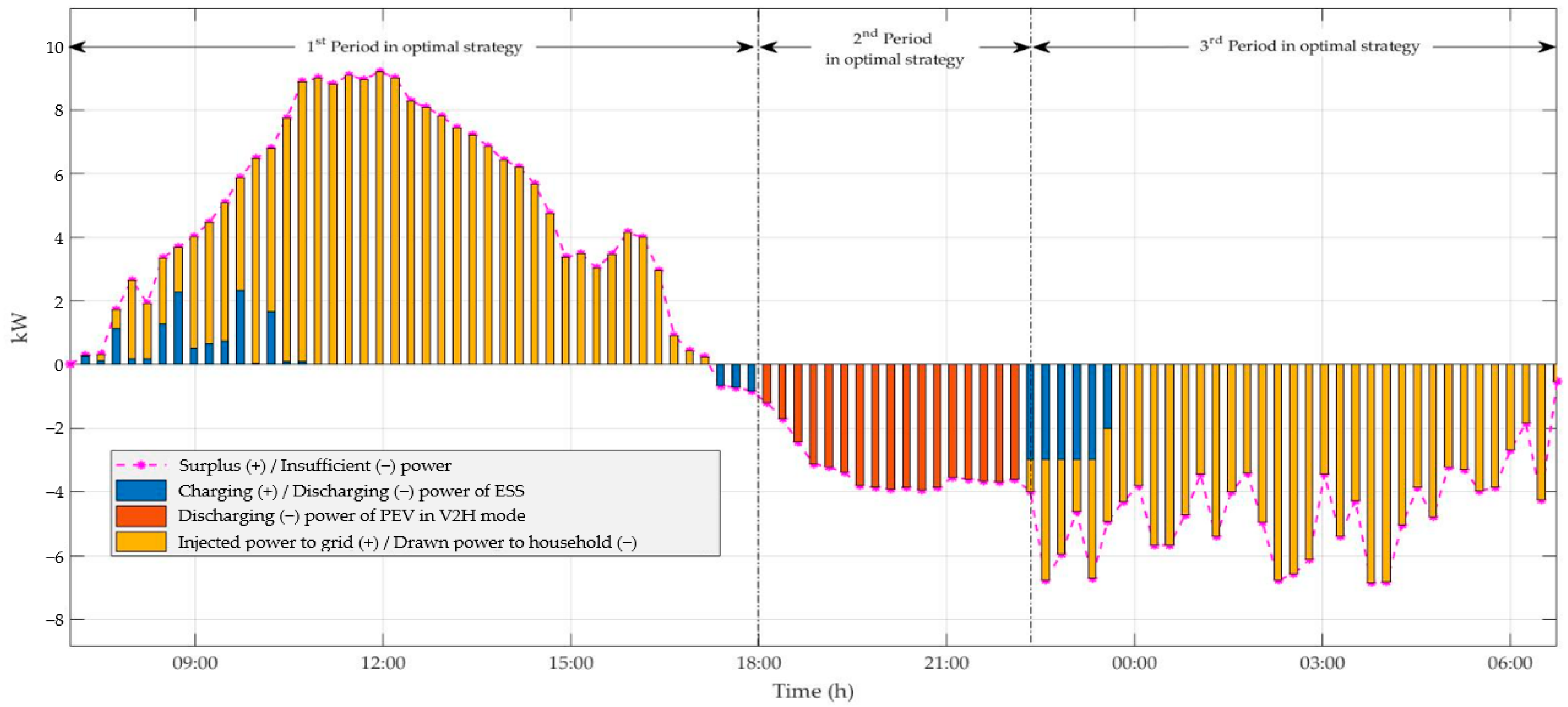
4.2. The Results of the Proposed Home Energy Management Strategy

The PV system power generation and the household load during each time slot are demonstrated in Figure 4. The PV system can generate power from 04:00 a.m. to 08:15 p.m. The maximum power rating is equal to 6.9000 kW from 02:00 a.m. to 07:00 a.m. Three periods are defined as follows: the first period is from 07:00 a.m. to 06:00 p.m., the second period is from 06:00 p.m. to 02:00 a.m. of the next day, and the third period is from 02:00 a.m. to 07:00 a.m.—the charging power of the PEV is combined with the household load in this period.

The surplus/insufficient power in the household and the charging/discharging power of the ESS and the PEV in V2H mode, $P_{\mathrm{G}}(t)$, are shown in Figure 5. In the first period, the surplus/insufficient power is calculated using Equation (1). When there is surplus power in the household, the ESS is charged following Equation (5). Afterward, the surplus power is injected into the grid following Equation (18). When there is insufficient power in the household, the ESS is discharged following Equation (6). Afterward, the power is drawn from the grid following Equation (18). In the second period, the PEV is operated in the V2H mode to support the ESS discharging, following Equation (12). In the third period, because the PEV operates as a load, there is more insufficient power than in the other periods. The surplus/insufficient power is calculated using Equation (2), When there is insufficient power in the household, the ESS is discharged following Equation (6). Afterward, the insufficient power is drawn from the grid following Equation (18).

The charging/discharging and stored energy for the PEV in each time slot is illustrated in Figure 6. In the first period, the stored energy of the PEV decreases according to the energy consumption (kWh/km) and the distance (km) traveled. In the second period, the PEV operates in the V2H mode to support the ESS operation. When there is insufficient power in the household, the PEV power is used following Equation (12). The stored energy of the PEV will continuously decrease until the stored energy of PEV is at 30% of its maximum capacity. After that, the PEV will not be discharged even if there is insufficient power in the household. Thus, the PEV $P_{\mathrm{G}}(t)$ decreases during the peak period and thus reduces the electrical energy costs for the consumer. In the third period, the PEV is charged using Equation (15). Consequently, the stored energy of the PEV will increase until it is more than 80% of its maximum capacity at 06:45 a.m. following the inequality constraint in Equation (27) and charging the PEV enough for traveling during the day.

The charging/discharging power and stored energy of ESS for each time slot are illustrated in Figure 7. In the first period, if there is a lot of surplus power in the household, the ESS will be charged using Equation (5). The stored energy of the ESS will reach 80% of its maximum capacity. The ESS will supply power when there is insufficient power in the household. In the second period, after the stored energy of the PEV is less than 30% of its maximum capacity, the ESS will discharge to supply power to the load using Equation (6). The stored energy of the ESS will discharge until the ESS energy is equal to 20% of its maximum capacity. In the third period, because the stored capacity of the ESS is equal to 20% of its maximum capacity, the ESS will not discharge even though there is insufficient power in the household during this period.

The daily electrical energy cost for the consumer during each time slot is shown in Figure 8. In the first period, because there is surplus power, the consumer can sell this surplus power to the grid. Therefore, the consumer earns revenue by injecting electric energy into the grid and, thus, reducing the daily electrical energy cost. In the second period, after storing energy, the ESS and PEV are decreased to their minimum capacities and the ESS and PEV power cannot be discharged to supply the household load. Consequently, the consumer has to purchase $P_{\mathrm{G}}(t)$. Therefore, the daily electrical energy cost for the consumer will continuously decrease. In the third period, the consumer has to purchase $P_{\mathrm{G}}(t)$ because the stored energy in the ESS and PEV are decreased to their minimum capacities. Therefore, the daily electrical energy cost for the consumer will continuously decrease. Finally, the daily electrical energy cost for the consumer is calculated, which is equal to −2.7197 USD. In other words, the consumer has to disburse the electrical energy cost to the utility grid equal to 2.7197 USD for a day.

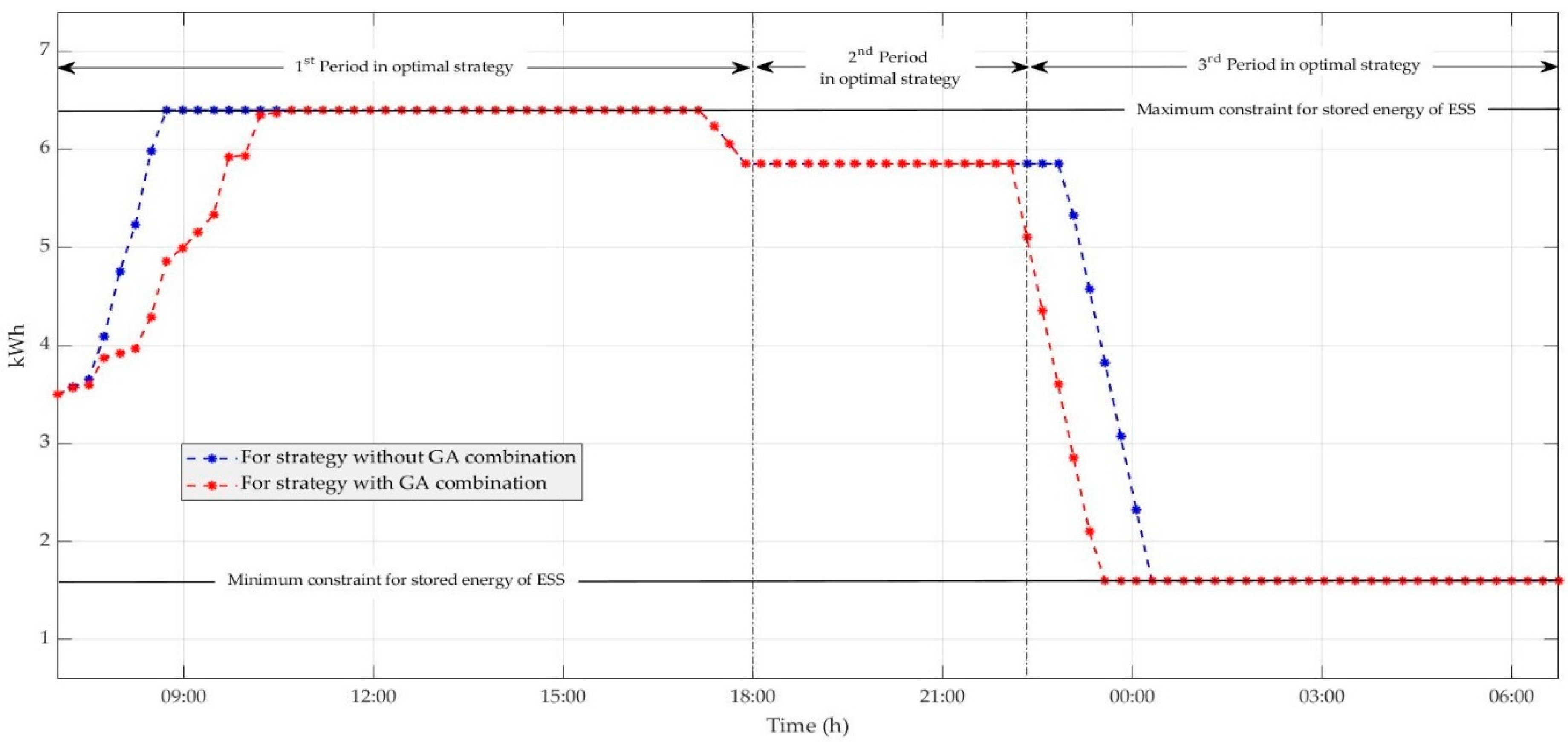
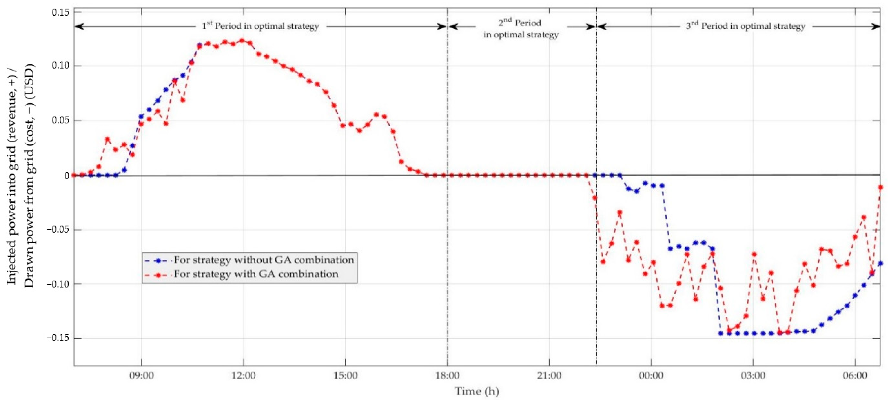
4.3. The Comparison Results between Home Energy Management Strategies with and without the Genetic Algorithm Combination

In this subsection, the results from the earlier method and the proposed optimal home energy management strategies are compared. The separated periods in the optimal strategy are defined as follows: the first period is from 07:00 a.m. to 06:00 p.m., the second period is from 06:00 p.m. to 10:00 p.m., and the third period is from 10:00 p.m. to 07:00 a.m. The combination of the strategy and the GA influenced the PEV and ESS operations and trading power between the household and the grid. Therefore, the electrical energy cost for the consumer changed following the optimization mechanism.

The PV system power generation and the household load during each time slot are demonstrated in Figure 9. The PV system can generate power from 04:00 a.m. to 08:15 p.m. The peak household load is equal to 6.8389 kW at 06:45 a.m.

The surplus/insufficient power in the household, the optimal charging/discharging power of the ESS and PEV in the V2H mode and the optimal $P_{\mathrm{G}}(t)$ are illustrated in Figure 10. In the first period, the surplus/insufficient power is calculated using Equation (1). When there is surplus power in the household, the ESS is charged according to the GA mechanism under the inequality constraint in Equation (29). Afterward, the surplus power is injected into the grid following Equation (18). When there is insufficient power in the household, ESS is discharged following Equation (6). Afterward, the power is drawn from the grid following Equation (15). In the second period, PEV is operated in the V2H mode to support the ESS discharging, following Equation (12). In the third period, the PEV is operated as a load. The PEV is charged according to the GA mechanism under the inequality constraints in Equation (31). The degree of insufficient power is calculated using Equation (2). When there is insufficient power in the household, the ESS power is discharged following Equation (6). Afterward, the insufficient power is drawn from the grid by Equation (19).

The charging/discharging power of the ESS and stored energy of the ESS obtained from the home energy management strategies with and without the GA are shown in Figure 11 and Figure 12, respectively. For the case using the optimal home energy management strategy, when there is surplus power in the household, the ESS is charged according to the GA mechanism under the inequality constraint in Equation (29). A comparison of the stored energy of the ESS with and without the GA combination is shown in Figure 11. When the stored energy of the ESS is equal to 80% of its maximum capacity, the ESS power will not be charged even if there is surplus power in the household during this period. When there is insufficient power in the household, the ESS power is discharged using Equation (6). However, during the second and third periods, the optimal strategy time slots for discharging are different from the discharging time slots estimated using the strategy without the use of GA. The ESS power is discharged again for supplying power to the household load and the PEV in the third period. When the stored energy of the ESS is equal to 20% of its maximum capacity, the ESS power will stop discharging even if there is insufficient power in the household during this period.

The charging/discharging power of the PEV and its stored energy obtained from the home energy management strategies with and without the GA combination are illustrated in Figure 13 and Figure 14, respectively. During the first period, the stored energy of the PEV decreases following the energy consumption rate (kWh/km) and the daily driven distance (km). The results are the same for both strategies with and without the GA combination. In the second period, the PEV operates in the V2H mode to support the ESS discharging, following Equation (12). Hence, the stored energy continuously decreases. In the third period, the PEV operates as a load that is optimally charged according to the GA mechanism, following the inequality constraints in Equation (31). The stored energy of the PEV will continuously increase until it is above 80% of its maximum capacity at 06:45 a.m. the next day, following the inequality constraint in Equation (27). The PEV charge should be enough for traveling during the day.

The $P_{\mathrm{G}}(t)$ obtained from the home energy management strategies with and without the GA combination are presented in Figure 15. During the first period, because the solar PV system generates more power than the household demand, and the stored energy of the ESS is sufficient to meet the household demand, the consumer can sell the surplus power to the grid. However, since the ESS is charged by the GA mechanism under the inequality constraint in Equation (29), the interaction powers that are calculated using Equation (15) will be different compared to the results using the strategy without the GA combination. In the second period, because the PEV operates in the V2H mode and can sufficiently meet the household demand, the consumer does not have to purchase $P_{\mathrm{G}}(t).$ In the third period, the consumer has to purchase $P_{\mathrm{G}}(t)$ to meet the household demand and optimally charge the PEV following Equation (19). Again, the results are different when compared to the results using strategy without the GA combination.

The electrical energy costs of the consumer obtained from the home energy management strategies with and without the GA combination are shown in Figure 16. Using the optimal strategy, $P_G(t)$ is different due to the optimal ESS and PEV charging mechanisms. Therefore, the estimated optimal electrical energy cost for the consumer is different using Equation (20). Finally, the daily electrical energy cost for the consumer was calculated, equaling −2.7197 USD. In other words, the consumer has to pay an electrical energy cost to the utility grid that is equal to 2.7197 USD for a day.

The comparison of the results obtained from the home energy management strategies with and without GA combination is presented in

Table 3. Comparison of the results between using strategies with and without the GA.

Scenarios of Home Energy Management Strategy	Power (kW)	Cumulative Energy (kWh)		Cumulative Revenue/Cost (USD)		Net Cost (USD)
	Peak Load	Injected to Grid	Drawn from Grid	Revenue	Cost	Daily Cost
Without GA	6.9000	53.0628	58.3542	2.6968	3.0815	0.3847
With GA	6.8389	53.0628	55.1235	2.6968	3.0545	0.3577
% Increment	-	-	-	-	-	-
% Reduction	0.8855	-	5.5364	-	0.8762	7.0185

. The strategy with the GA can decrease the cumulative drawn energy from the grid from 58.3542 kWh to 55.1235 kWh. Therefore, the cumulative cost for the consumer is decreased from 3.0815 USD to 3.0545 USD. In consequence, the daily electrical energy cost for the consumer is decreased from 0.3847 USD to 0.3577 USD. Moreover, the strategy with the GA can equalize the household load in the third period and decreases the peak household load from 6.9000 kW to 6.8389 kW; consequently, the utility grid does not have to supply high power to the household for a long time.

In summary, from Table 3, the results obtained from the strategy with the GA show that the cumulative energy drawn from the grid decreases by 5.5364%, the cumulative cost for the consumer decreases by 0.8762%, and the peak household load decreases by 0.7072% compared to the results obtained from the strategy without the GA. Finally, the daily electrical energy cost for the consumer decreases by 7.0185% compared to the results obtained from the strategy without the GA. The GA can only be added to the charging processes for the ESS and PEV for minimizing the daily cost. For the discharging processes of the ESS and PEV, the GA is not useful to be added because the proposed strategy already controlled the discharged power at the maximum value to decrease the purchasing power from the grid. As a result, the difference between the results of the strategies with and without the GA is not significant. However, because the results were simulated only for a day, the authors strongly believe that the monthly or yearly electrical energy cost for consumers using the strategy with the GA will be significantly reduced.

For the computation time comparison, the calculation time of the proposed home energy management strategy without the GA is 0.3505 s. On the other hand, the calculation time of the proposed home energy management strategy with the GA is 4,217.6579 s or 1 h 10 min 17.6579 s. It can be seen that the computation times of the two methods are reasonable for applying in day-ahead planning.

5. Conclusions

This paper presents the optimal home energy management strategy based on a solar PV system, a PEV, and an ESS in a household considering the power usage under TOU tariffs. The TOU tariffs of Thailand were used for electrical energy cost calculations in this study. The charging/discharging powers of ESS and PEV, $P_{\mathrm{G}}(t)$, are managed by the proposed strategy. To increase the capability of the strategy, the meta-heuristic optimization using a genetic algorithm was integrated with the proposed home energy management strategy.

To confirm the improved performance of the proposed strategy, the home energy management strategies with and without the GA combinations were evaluated using MATLAB-based numerical simulation results. The strategy without the GA combination was applied by carefully dividing the day into three time periods. The results present the daily solar power generation, household load profile, and surplus/insufficient power, which, in turn, triggered the PEV and ESS operations during each time slot. Finally, the daily electrical energy cost for the consumer was calculated.

In the case of using the strategy without the GA, the simulation results show that the consumer has to pay a daily electrical energy rate to the utility grid equal to 0.3847 USD. However, the case of using the strategy with the GA combination can decrease the cumulative energy drawn from the grid from 58.3542 kWh to 55.1235 kWh. Therefore, the cumulative energy cost for the consumer decreases from 3.0815 USD to 3.0545 USD. In consequence, the daily or net electrical energy cost for the consumer decreases from 0.3847 USD to 0.3577 USD. Moreover, the strategy with the GA combination can equalize the household load in the third period and decreases the peak household load from 6.9000 kW to 6.8389 kW; consequently, the utility grid does not need to supply a lot of power to the household for a long time.

In summary, the proposed optimal home energy management strategy can provide the optimal charging power of an ESS and a PEV, and optimal power interactions between the grid and a household. The comparison of the results between the proposed home energy management strategy with and without the GA can be summarized as follows:

• The cumulative drawn energy from the grid decreases by 5.5364%.
• The cumulative energy cost for the consumer decreases by 0.8762%.
• The daily electrical energy cost for the consumer decreases by 7.0185%

However, from the simulation results, the household peak load was still high, which can cause high investment costs of the utility grid in the development of the main grid; therefore, future works should take the household peak load reduction into account. Finally, the optimal sizing of the ESS should be considered in order to completely maximize the benefits of using the ESS. Moreover, nowadays, the Harris hawks optimization (HHO) [29] and water cycle algorithm (WCA) [30] are popular because they perform better than other traditional meta-heuristics algorithms, such as the GA. This is a significant research gap that can improve this research work in the future.

References

1. International Energy Agency (IEA). Global EV Outlook 2019-Scaling-Up the Transition to Electric Mobility. Available online: https://www.iea.org/reports/global-ev-outlook-2019 (accessed on 25 March 2021).
2. Ministry of Energy, International Renewable Energy Agency (IRENA). Renewable Energy Outlook: Thailand. 104. Available online: https://www.irena.org/-/media/files/irena/agency/publication/2017/nov/irena_outlook_thailand_2017.pdf (accessed on 25 March 2021).
3. Available online: www.eppo.go.th/index.php/th/eppo-intranet/item/12438-ev-plan (accessed on 25 March 2021).
4. Srithapon, C.; Ghosh, P.; Siritaratiwat, A.; Chatthaworn, R. Optimization of Electric Vehicle Charging Scheduling in Urban Village Networks Considering Energy Arbitrage and Distribution Cost. Energies 2020, 13, 349. [Google Scholar] [CrossRef] [Green Version]
5. Denholm, P.; O’Connell, M.; Brinkman, G.; Jorgenson, J. Overgeneration from Solar Energy in California. A Field Guide to the Duck Chart; Technical Report NREL/TP-6A20-65023; National Renewable Energy Laboratory: Golden, CO, USA, 2015. [Google Scholar]
6. Datta, U.; Kalam, A.; Shi, J. Electric Vehicle (EV) in Home Energy Management to Reduce Daily Electricity Costs of Residential Customer. J. Sci. Ind. Res. 2018, 77, 559–565. [Google Scholar]
7. Khemakhem, S.; Rekik, M.; Krichen, L. Double Layer Home Energy Supervision Strategies Based on Demand Response and Plug-in Electric Vehicle Control for Flattening Power Load Curves in a Smart Grid. Energy 2019, 167, 312–324. [Google Scholar] [CrossRef]
8. Rana, R.; Prakash, S.; Mishra, S. Energy Management of Electric Vehicle Integrated Home in a Time-of-Day Regime. IEEE Trans. Transp. Electrif. 2018, 4, 804–816. [Google Scholar] [CrossRef]
9. Tushar, M.H.K.; Zeineddine, A.W.; Assi, C. Demand-Side Management by Regulating Charging and Discharging of the EV, ESS, and Utilizing Renewable Energy. IEEE Trans. Ind. Inform. 2018, 14, 117–126. [Google Scholar] [CrossRef]
10. Chowdhury, N.; Hossain, C.A.; Longo, M.; Yaïci, W. Optimization of Solar Energy System for the Electric Vehicle at University Campus in Dhaka, Bangladesh. Energies 2018, 11, 2433. [Google Scholar] [CrossRef] [Green Version]
11. Hossain, C.; Chowdhury, N.; Longo, M.; Yaïci, W. System and Cost Analysis of Stand-Alone Solar Home System Applied to a Developing Country. Sustainability 2019, 11, 1403. [Google Scholar] [CrossRef] [Green Version]
12. Fachrizal, R.; Munkhammar, J. Improved Photovoltaic Self-Consumption in Residential Buildings with Distributed and Centralized Smart Charging of Electric Vehicles. Energies 2020, 13, 1153. [Google Scholar] [CrossRef] [Green Version]
13. Khalid, M.; Ahmadi, A.; Savkin, A.; Agelidis, V. Minimizing the Energy Cost for Microgrids Integrated with Renewable Energy Resources and Conventional Generation Using Controlled Battery Energy Storage. Renew. Energy 2016, 97, 646–655. [Google Scholar] [CrossRef]
14. Van Der Meer, D.; Chandra Mouli, G.R.; Morales-España Mouli, G.; Elizondo, L.R.; Bauer, P. Energy Management System With PV Power Forecast to Optimally Charge EVs at the Workplace. IEEE Trans. Ind. Inform. 2018, 14, 311–320. [Google Scholar] [CrossRef] [Green Version]
15. Abdalla, M.A.A.; Min, W.; Mohammed, O.A.A. Two-Stage Energy Management Strategy of EV and PV Integrated Smart Home to Minimize Electricity Cost and Flatten Power Load Profile. Energies 2020, 13, 6387. [Google Scholar] [CrossRef]
16. Yang, X.; Zhang, Y.; Zhao, B.; Huang, F.; Chen, Y.; Ren, S. Optimal Energy Flow Control Strategy for a Residential Energy Local Network Combined with Demand-Side Management and Real-Time Pricing. Energy Build. 2017, 150, 177–188. [Google Scholar] [CrossRef]
17. Khan, Z.A.; Zafar, A.; Javaid, S.; Aslam, S.; Rahim, M.H.; Javaid, N. Hybrid Meta-Heuristic Optimization Based Home Energy Management System in Smart Grid. J. Ambient. Intell. Hum. Comput. 2019, 10, 4837–4853. [Google Scholar] [CrossRef]
18. Yang, J.; Liu, J.; Zilu, F.; Weiting, L. Electricity Scheduling Strategy for Home Energy Management System with Renewable Energy and Battery Storage: A Case Study. IET Renew. Power Gener. 2017, 12, 639–648. [Google Scholar] [CrossRef]
19. Olsen, J.; Sarker, R.; Ortega-Vazquez, A. Optimal Penetration of Home Energy Management Systems in Distribution Networks Considering Transformer Aging. IEEE Trans. Smart Grid 2018, 9, 3330–3340. [Google Scholar] [CrossRef]
20. Lee, S.; Choi, D.-H. Energy Management of Smart Home with Home Appliances, Energy Storage System and Electric Vehicle: A Hierarchical Deep Reinforcement Learning Approach. Sensors 2020, 20, 2157. [Google Scholar] [CrossRef] [PubMed] [Green Version]
21. Turker, H.; Colak, I. Multiobjective Optimization of Grid- Photovoltaic- Electric Vehicle Hybrid System in Smart Building with Vehicle-to-Grid (V2G) Concept. In Proceedings of the 2018 7th International Conference on Renewable Energy Re-search and Applications (ICRERA), Paris, France, 14–17 October 2018; pp. 1477–1482. [Google Scholar]
22. Wu, X.; Hu, X.; Yin, X.; Moura, S.J. Stochastic Optimal Energy Management of Smart Home With PEV Energy Storage. IEEE Trans. Smart Grid 2018, 9, 2065–2075. [Google Scholar] [CrossRef]
23. Aznavi, S.; Fajri, P.; Asrari, A.; Harirchi, F. Realistic and Intelligent Management of Connected Storage Devices in Future Smart Homes Considering Energy Price Tag. IEEE Trans. Ind. Appl. 2020, 56, 1679–1689. [Google Scholar] [CrossRef]
24. Hou, X.; Wang, J.; Huang, T.; Wang, T.; Wang, P. Smart Home Energy Management Optimization Method Considering Energy Storage and Electric Vehicle. IEEE Access 2019, 7, 144010–144020. [Google Scholar] [CrossRef]
25. Provincial Electricity Authority (PEA), Thailand. Available online: https://www.pea.co.th/en (accessed on 25 March 2021).
26. European Network of Transmission System Operators. Available online: https://transparency.entsoe.eu/generation/ (accessed on 25 March 2021).
27. Provincial Electricity Authority (PEA), Thailand. Available online: https://www.pea.co.th/Portals/0/Document/connection_code_2016_20170928.pdf (accessed on 25 March 2021).
28. Electricity-Tarif 2018, Provincial Electricity Authority (PEA), Thailand. Available online: https://www.pea.co.th/en/electricity-tariffs (accessed on 14 May 2021).
29. Helmi, A.M.; Carli, R.; Dotoli, M.; Ramadan, H.S. Efficient and Sustainable Reconfiguration of Distribution Networks via Metaheuristic Optimization. IEEE Trans. Autom. Sci. Eng. 2021, 19, 1–17. [Google Scholar] [CrossRef]
30. Muhammad, M.A.; Mokhlis, H.; Naidu, K.; Amin, A.; Franco, J.F.; Othman, M. Distribution Network Planning Enhancement via Network Reconfiguration and DG Integration Using Dataset Approach and Water Cycle Algorithm. J. Mod. Power Syst. Clean Energy 2020, 8, 86–93. [Google Scholar] [CrossRef]
Figure 1. The typical home energy management system (HEMS) model.
Energies 15 00537 g001
Figure 2. The steps of the proposed home energy management strategy.
Energies 15 00537 g002
Figure 3. The process of the proposed optimal home energy management strategy.
Energies 15 00537 g003
Figure 4. Daily power generation of the solar PV system and household load profile.
Energies 15 00537 g004
Figure 5. Energy management results of the strategy without GA when there is surplus and insufficient power in a household in each time slot.
Energies 15 00537 g005
Figure 6. The charging (+)/discharging (−) power and stored energy of the PEV in each time slot.
Energies 15 00537 g006
Figure 7. The charging (+)/discharging (−) and stored energy for the ESS in each time slot.
Energies 15 00537 g007
Figure 8. The electrical energy cost of each time slot and daily electrical energy cost for the consumer.
Energies 15 00537 g008
Figure 9. Daily power generation of the solar PV system and household load profile.
Energies 15 00537 g009
Figure 10. Optimal energy management results of the strategy with GA when there is surplus and insufficient power in a household in each time slot.
Energies 15 00537 g010
Figure 11. Comparison of charging (+)/discharging (−) power of the ESS using strategies with and without the GA.
Energies 15 00537 g011
Figure 12. Comparison of stored energy of the ESS using strategies with and without the GA.
Energies 15 00537 g012
Figure 13. Comparison of charging (+)/discharging (−) power of the PEV using strategies with and without the GA.
Energies 15 00537 g013
Figure 14. Comparison of stored energy of the PEV using strategies with and without the GA.
Energies 15 00537 g014
Figure 15. Comparison of interaction powers using strategies with and without the GA.
Energies 15 00537 g015
Figure 16. Comparison of energy costs of the consumer using strategies with and without GA.
Energies 15 00537 g016