
Agent-Based Modelling of Urban District Energy System Decarbonisation—A Systematic Literature Review


1
Energy Economics Group, Technische Universität Wien, Karlsplatz 13, A-1040 Vienna, Austria
2
Dipartimento Ambiente Costruzioni e Design, Scuola Universitaria Professionale Della Svizzera Italiana (SUPSI), Via Francesco Catenazzi 23, CH-6850 Mendrisio, Switzerland
*
Author to whom correspondence should be addressed.
†
Current address: Lawrence Berkeley National Laboratory, 1 Cyclotron Rd, Berkeley, CA 94720, USA.
Energies 2022, 15(2), 554; https://doi.org/10.3390/en15020554
Submission received: 7 December 2021
/
Revised: 29 December 2021
/
Accepted: 30 December 2021
/
Published: 13 January 2022
Abstract
:There is an increased interest in the district-scale energy transition within interdisciplinary research community. Agent-based modelling presents a suitable approach to address variety of questions related to policies, technologies, processes, and the different stakeholder roles that can foster such transition. However, it is a largely complex and versatile methodology which hinders its broader uptake by researchers as well as improved results. This state-of-the-art review focuses on the application of agent-based modelling for exploring policy interventions that facilitate the decarbonisation (i.e., energy transition) of districts and neighbourhoods while considering stakeholders’ social characteristics and interactions. We systematically select and analyse peer-reviewed literature and discuss the key modelling aspects, such as model purpose, agents and decision-making logic, spatial and temporal aspects, and empirical grounding. The analysis reveals that the most established agent-based models’ focus on innovation diffusion (e.g., adoption of solar panels) and dissemination of energy-saving behaviour among a group of buildings in urban areas. We see a considerable gap in exploring the decisions and interactions of agents other than residential households, such as commercial and even industrial energy consumers (and prosumers). Moreover, measures such as building retrofits and conversion to district energy systems involve many stakeholders and complex interactions between them that up to now have hardly been represented in the agent-based modelling environment. Hence, this work contributes to better understanding and further improving the research on transition towards decarbonised society.
1. Introduction
Deep decarbonisation of the building sector in the EU is one of the key prerequisites for becoming climate neutral by 2050, as buildings account for around 40% of final energy consumption [1]. In this regard, “zero energy” building concepts, which largely rely on reduced energy demand and on-site renewable generation, have recently gained considerable interest in both scientific literature [2,3,4,5,6,7] and in practice [8]. However, some researchers argue that dense and compact buildings on small plots have a small potential for an on-site renewable generation [2,9] and can hardly achieve zero energy balance. Thus, the expansion of building-level “zero energy” concept to the scale of neighbourhoods, districts and communities is a potential alternative solution. With this motivation, several concepts that aim to achieve zero or positive energy balance, such as Net-Zero Energy Neighbourhoods (or Districts) [2,4,10], Plus-Energy Quarters [11,12], and Positive Energy Districts [13,14,15] are being implemented currently.
Increased interest in such neighbourhood or district-level concepts as a solution for energy and climate issues, raise a multitude of new questions, the most generic of them being: “what socio-techno-economic conditions support the transition of urban districts towards zero and positive energy districts?”. More concretely, what policies, technologies and processes can foster this transition? In this context, it is becoming even more critical to understand the perspectives and roles of various stakeholders, including households, firms and public institutions, as their participation (e.g., via energy conservation, prosumption and energy trading, infrastructure development) in transitioning to a decarbonised society can be supported by well-designed and inclusive policies and programs [16,17].
Within a broad selection of models used in energy system analysis [18], Agent-based Modelling (ABM) approach is distinguished by its ability to represent individual decision-making of heterogeneous actors, as well as interactions between them [19,20]. Moreover, it is a simulation-type model that allows defining micro-level action and interaction rules, leading to macro-level emergent insights [21]. Hence, it is deemed suitable for exploring policy-related “what-if” questions and incorporating actors’ perspectives in the energy system [16,17,22].
This article aims to obtain an overview of how ABM has been used to model policy interventions that facilitate the decarbonisation (i.e., energy transition) of building-related urban district energy systems and consider stakeholders’ social characteristics and interactions. We use systematic literature review (SLR) to select the studies and discuss critically the important aspects of ABMs, such as modelling choices and agent characterisation. Hence, this SLR serves as a starting point for those who want to understand how ABM can simulate urban district-level energy transition and contributes with:
- A detailed insight on how ABM has been used in modelling urban district’s (building-related) energy systems while considering stakeholders and policies;
- A discussion of modelling choices and methodologies;
- Identification of research gaps and potential application streams.
This paper is structured as follows. Section 2 provides the context to this research topic by defining urban district energy systems and summarising the previous research on applying ABM to model energy systems. It is followed by the description of our approach for the systematic selection and review of the articles in Section 3. The main results of the review are presented in Section 4 and organised in different thematic subsections related to essential aspects of ABMs of urban district energy systems, namely: model purpose and outputs, agents, their decision-making and interaction rules, technologies and policies covered, spatial and temporal aspects, as well as experimental setup of simulations, use of empirical data, and implementation platform used. The paper is finalised with synthesised observations and future research suggestions in Section 5.
2. Background and Definitions
In this section, we lay down the foundations for the topic of our focus. Namely, we want to refer to the existing literature and define the urban district energy system. Secondly, we discuss the state-of-the-art of ABM’s application in the energy systems research.
2.1. Urban District Energy Systems and Models
The energy system is defined by the IPCC [23] as: “all components related to the production, conversion, delivery, and use of energy”. The energy system is also seen as a socio-technical system, comprised of more than just technical components, but also markets, institutions, consumer behaviours and other factors that affect the construction and operation of technical infrastructures [24].
The differentiation of energy systems into “urban” and “district” is generally about defining the system’s scope. In Europe, “urban areas” refer to cities (i.e., densely populated areas), towns and suburbs (i.e., intermediate density areas), as opposed to rural (i.e., sparsely populated) areas [25]. According to the motivation and purpose of this work, we look at the studies that address the energy system challenges of densely populated urban areas.
Depending on various national contexts, “districts” and “neighbourhoods” can denote different administrative and non-administrative areas of cities or countries. Like [6,7,26], we do not refer to certain juridical or administrative areas, but as part of an urban area. Hence, everything from a small to a large group of buildings is considered a “district” within this work. Due to the inconsistent use of the similar terms in the literature, the synonyms of “district” such as “neighbourhood”, “quarter”, “block” and “community” are included in the analysis.
It is important to note though, that the search for “district energy systems” brings to district-scale energy systems, be that traditional district-level thermal and hybrid energy systems (e.g., cogeneration) [27,28,29,30] or distributed energy systems such as PV, solar thermal, battery storage [31,32,33,34]. However, consistent with the above-mentioned definitions of [23,24], we keep the scope of “district energy system” broader and do not limit it to the technical components only.
There are various energy system modelling approaches and tools that can be or are used at the district-scale for different purposes [24,31,34]. As [31] conclude about the numerous urban district-level energy models and tools: “some tools aim to provide a single simulation that addresses many issues, while others give detailed results regarding specific parts of the system”. Although the advantages of ABM in studying complex systems and enabling the analysis of policies are acknowledged [17,24,35,36,37], its role in studying district energy systems, to the authors’ knowledge, has not yet been explored in detail.
2.2. Agent-Based Modelling in Energy Systems Research
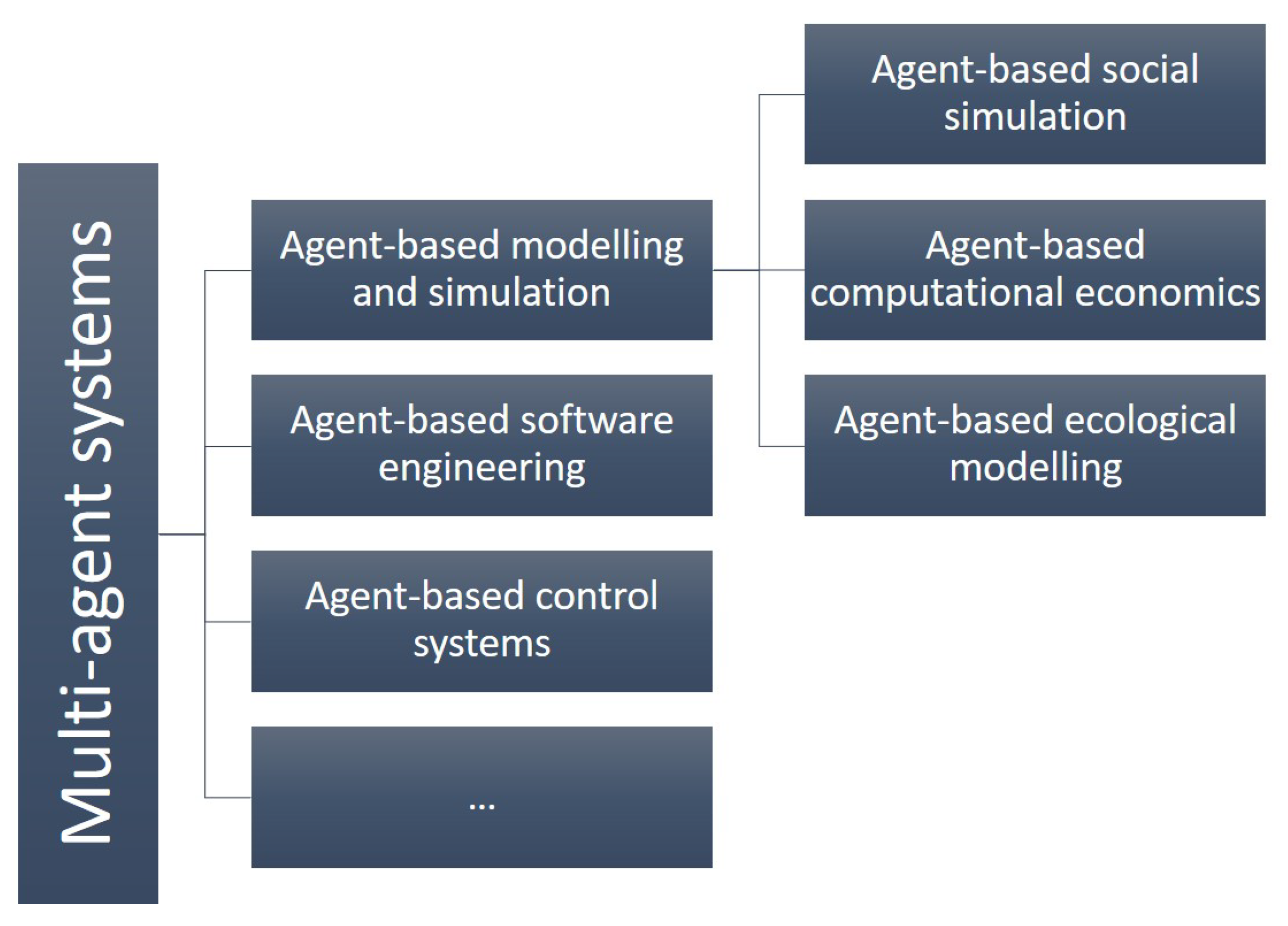
ABM is a modelling approach that can be seen as one of the applications of a software engineering paradigm named “Multi-agent systems” (MAS) [38]. (Some application fields of MAS are represented in Figure 1). There is an ambiguity between MAS and ABM. However, the general understanding is that MAS is an overarching architecture or paradigm, which, when applied for simulating various phenomena by abstracting real-life systems (e.g., human, animals, organisations) is usually called ABM or Agent-Based Simulation (ABS). Whereas MAS-based engineering deals with applying the MAS architecture to create a software or control system, ABM applies MAS paradigm to draw implications about other systems (e.g., human settlements, stock markets, etc.). The common point between MAS-based engineering and ABM is in the desire to understand a complex system by assuming a distributed or autonomous behaviour instead of centralised or equation-governed behaviour of system elements (e.g., like in System Dynamics approach). Hence, the terms “multi-agent-system”, “multi-agent-based-modelling” and “agent-based modelling” are sometimes used interchangeably in the literature [39,40,41,42]. However, the difference of these two approaches, namely that ABM sets up agents with characteristics of real-world analogy to see what happens when they act, while in a multi-agent system, agents are defined with certain characteristics, connections and choices, such that they achieve specified emergent states [43].
ABM can, thus, be more specifically understood as a computer simulation of an artificial world populated by agents—discrete decision-making entities (individual, household, firm, etc.)—whose behaviours and rules of different complexity can govern interactions. One of the main reasons for choosing ABM over traditional equation-based modelling approaches in energy systems analysis (i.e., system dynamics, optimisation models, computable general equilibrium models) is its ability to incorporate heterogeneity and adaptivity of energy consumers [45]. In the energy system research, this strength has been exploited for: (a) analysing the demand side of energy system [17], e.g., incorporating occupant behaviour in buildings [46,47]; (b) better-informing policy-making and infrastructure planning [22,36], e.g., determining target groups for interventions [48,49] or recommendations specific to the adoption of particular renewable energy or energy-efficient technologies [3,50,51].
As the number and publication date of review papers indicate (see Table A1 in Appendix A), the first applications of ABM in energy research were for representing wholesale electricity markets to analyse market structures [45]. The possibility of using ABM for questions related to smart electricity grids and markets, such as the integration of demand response and distributed generation in local or centralised markets, is explored by [44]. The potential of ABM to improve our understanding of consumer energy demand, by allowing to account for social, behavioural, economic, technological, and market and policy factors that influence energy demand is presented by [17]. Questions that interest energy economists and policymakers are how consumers adopt energy-efficient technology and how to encourage them. The benefit that ABM can bring to this stream of research, as well as barriers and incentives for the adoption of energy-efficient measures in the residential sector are addressed by [22,36]. Though our review topic overlaps with theirs, we do not focus on the ABMs of “innovation diffusion” only and explore a wider range of approaches.
3. Methods
This work is based on the literature review type originating in biomedical and healthcare research and becoming prominent in energy system research too [35,36]—systematic literature review (SLR).
The current SLR is carried out on the 13th of September, 2021 in the Scopus database only. The main research question thereby is: “how ABM has been applied in studying the urban district (building-related) energy systems?”. Accordingly, the search string provided in the PRISMA Flow diagram in Figure 2 reflects this question. First, the literature suggests many variations of agent-based concepts—simulations, models, approaches, as well as “multi-agent” and “multi-agent-based” simulations, models, and approaches. Although there are differences between MAS and ABM (see Section 2.2), they are sometimes used interchangeably in the literature. Therefore, the studies referring to “multi-agent-based” simulations were not excluded automatically but carefully checked. Second, the search term “energy OR heat*” ensures that all studies mentioning energy or heat are captured. Urban district energy systems are defined here as a group of buildings, heating and cooling infrastructure, distributed energy resources (PV, battery, solar thermal, heat pump, CHP), electricity distribution network, and energy producers, consumers, prosumers and other relevant stakeholders in a given district or city. Hence, we exclude, for example, transport-related studies, which returned 92 additional records in Scopus. Third, as explained in Section 2.1, "district” is used interchangeably with “neighbourhood”, “quarter”, “block”, “community”. Moreover, sometimes city or town-level models are applicable to a smaller scale too. Hence, we considered the article with at least one of the terms.
After a rigorous identification in the Scopus database and removing duplicated records, further screening was performed using Scopus automatic filtering, reading titles and abstracts. Journal and conference articles, written in English, accessible either openly or the research institution’s library, and relevant to the energy research were filtered out. Finally, full-text analysis has been applied to ensure the selected studies match the aim of this review. The exact reasons for exclusion together with the full SLR process are presented in Figure 2.
After the papers have been selected, they are qualitatively analysed based on the following key aspects of ABMs:
- model purpose and outputs (Section 4.1)
- agents (Section 4.2)
- agent decision rules (Section 4.3)
- agent interaction (Section 4.4)
- technologies and policies modelled (Section 4.5)
- spatial and temporal aspects (Section 4.6)
- empirical grounding (Section 4.7)
As already mentioned in one of the previous review articles [37], ABMs differ strongly in how they are designed and implemented, so a quantitative comparison of models is impractical. Therefore, we focused on the qualitative description of modelling choices and methodological aspects within the selected ABMs. The defined thematic clusters of analysis were inspired by the review approaches of [20,36], as well as by the Overview, Design Concepts, and Details (ODD) protocol [52,53,54]—the attempt to formalise the documentation of the ABM’s modelling process and results. Whenever included or implemented, the ODD protocol improves the readability and ensures that the information needed to understand and further analyse the models is present.
Within this work, we focus on the components of the energy system related to the built environment of a district (i.e., buildings, heating, cooling, electricity supply systems) and human individuals or groups. Thus, studies focusing on other sectors (i.e., transport, industry, or agriculture and forestry) and elements (e.g., energy markets, information systems, power network) of the energy system, though recognised as part of the energy system, are outside the scope of this review.
4. Results: ABMs of Urban District Energy Systems
This section presents the findings from the thorough analysis of 25 studies based on model purposes and outputs, agents, their decision-making frameworks and interactions, technologies and policies covered, spatial and temporal aspects, and empirical grounding.
4.1. Model Purposes and Outputs
The review by [17] highlights that ABM is well-suited to answer two kinds of energy-demand questions: those related to policy design and evaluation and those related to system design and infrastructure planning. The review process reflects the existence of these two motivations for modelling, of which we only focus on those that are relevant for policy design. These studies evaluate the agents’ behavioural response to external stimuli in the form of a policy, regulation, observation or feedback, and peer influence. Rai & Robinson [51] present a well-validated example of an ABM used to test the influence of the regulatory framework on adopting renewable technology. They examine how additional rebates (i.e., partial refund of an item’s cost) for low-income households and changes in the amount of rebate, affect the adoption of rooftop PV in Austin, Texas.
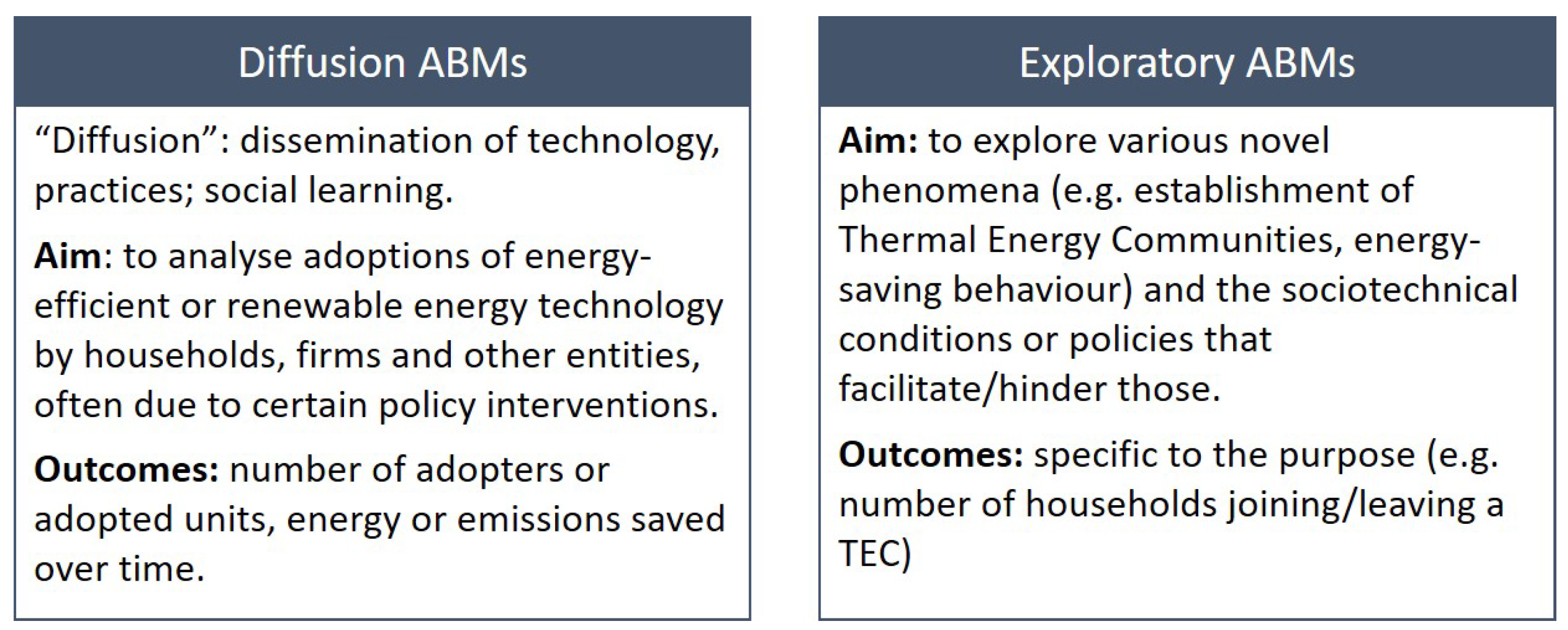
A model’s purpose or objective must be “clear, concise and specific” [52], which is essential for others to understand why some aspects of reality are included in a model while others are omitted. It is because each a model should be a “purposeful” abstraction of reality [55]. The purposes of the 25 selected models are diverse. However, we identified two main thematic clusters: diffusion and exploratory ABMs (see Figure 3).
One large thematic cluster is the exploration of technology adoption that has its foundations in innovation diffusion theories [56]. This type of ABM is often named “agent-based diffusion model” [22,36,56,57]. They aim to analyse adoptions of energy-efficient or renewable energy technology by households, firms and other entities, often due to certain policy interventions [3,51,58,59,60,61,62,63,64]. Usually, such models’ outputs are the number of adopters or adopted units, energy or emissions saved over time (see Table 1). This approach allows us to observe what factors affect the adoptions of technologies in which ways. The term “diffusion” encompasses concepts like social learning and dissemination [65]. Thus, this approach is also well-suited to represent the dissemination of energy-related practices and behaviours, such as energy-saving [47,49], energy-efficient ventilation behaviour [66,67], user learning (i.e., energy saving) after authoritative smart meter adoption [68], building renovation behaviour [69], weatherisation (i.e., making apartments weather-proof) [70], buying energy-efficient appliances and switching an energy provider [71]. Similar to technology adoption, these studies investigate how energy-related behaviours are adopted and how much energy can be saved. Three models [66,67,68] focus on both technology adoption and the resulting behaviour dissemination.
The remaining works have more exploratory purposes and are less established than diffusion ABMs. Fouladvand et al. [72] investigate how Thermal Energy Communities (TEC) can be formed and sustained, where agents can either join a new or existing community or decide to drop-out based on financial, technological and energy plan (e.g., self-consumption) evaluations. Busch et al.’s [73] model is distinguished from other models by representing the continuous process of engagement and district-heating development instead of instantaneous decisions (e.g., to adopt, to invest). In these studies, the output metrics are very specific to the purpose and subject studies (see Table 2).
4.2. Agents
Agent is a key element in this modelling approach. Many previous studies highlight that there is no common definition of an agent [44,78], as its properties depend on the model’s purpose and application area. Nevertheless, many authors refer to the following basic definition presented by [79]: “Agent is an encapsulated computer system that is situated in some environment, and that is capable of flexible, autonomous action in that environment in order to meet its design objectives”. In the ODD protocol, agents are one of the model’s “entities”, along with spatial units and the overall environment [54]. It is due to the parallels between the agent-based modelling approach and Object-Oriented Programming (OOP) (i.e., the ‘classes’ or its instances in OOP could be equivalent to ‘entities’ in ABM). It might lead to confusion among readers who are new to Agent-based modelling or use different implementation tools. In the current article, we differentiate between agents and other entities, where we refer to “agents” as autonomous entities that can make decisions (i.e., implement certain algorithms) and interact (i.e., obtain information from its environment or other agents) in order to reach its objectives.
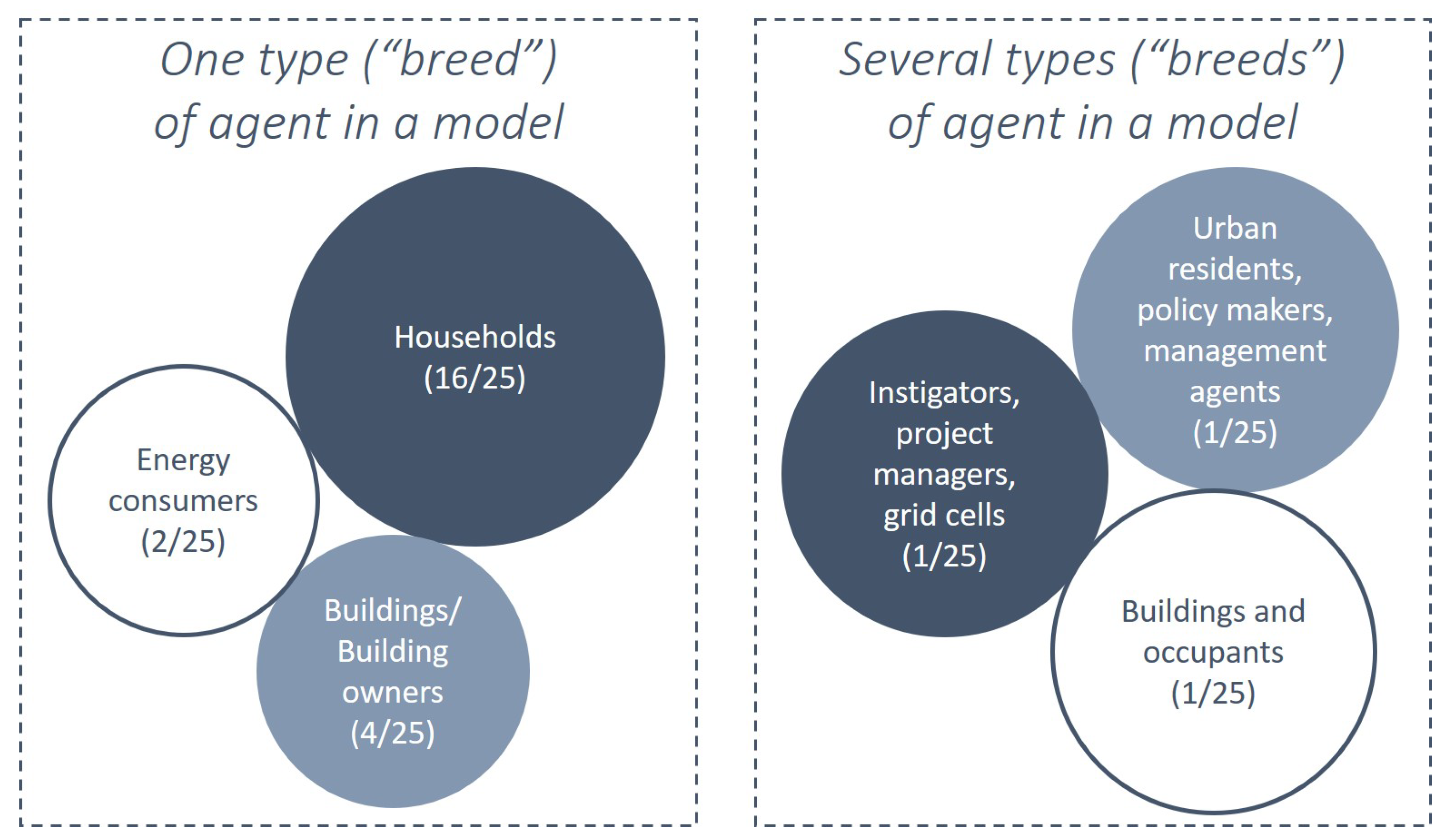
Most of the agents in the selected studies are “households” (15 out of 25) and three studies also denote them as “energy consumers” [3,68,71] (see Table 2). Since most of these studies model the adoption of PV or other technologies, “households” are most common decision-makers in this regard. Majority of these models limit their agent population to the households that live in a single-family building, because installation of renewable energy in other types of housing (rented apartments, multi-family housing) is subject to additional legal or physical constraints. However, few models are exceptions: [3,61] differentiate agents into tenants and house owners, where only house owners can buy and install PV and tenants can choose from green electricity or community solar program; Nava Guerrero et al. [76] attempts to represent group decision-making regarding heating system, insulation or RE system installation in multi-family houses. In other models, building (or building block) owner [60,69] and building agents [59] can make building-level decisions, i.e., adopting PV or renovation. The rationale of these models is that there is only one building owner that can make such a decision.
While the above-mentioned studies focus predominantly on one type of stakeholder, there are few models that involve different types of stakeholders as agents [73]. For example, in [73], instigator agents (i.e., local authorities, commercial, and community-based developers) are driving the development of projects, whereas “projects” are management agents responsible for carrying out actions on behalf of their parent instigators [73]. In models with multiple types of stakeholders, it is becoming more challenging to draw a line between agents and other entities, e.g., as in [47], as all of them are essentially realised as classes. However, one can observe the tendency to call human-like entities “agents”, e.g., instigator agents, and passive entities like grid cells and projects [73] as just “entities”. Figure 4 summarises the types of agents we identified in the reviewed models.
The essential part of ABMs is decision rules that govern the actions of agents. Decision rules are realised with the help of attributes that describe agents [43]. Moreover, interaction and social influence play a significant role in agent’s decision making. Hence, the following subsections give an overview of the decision-making rules and agent interaction strategies implemented in the reviewed models.
4.3. Agent Decision Rules
Decision-making rules (also called behavioural rules, decision rules or models, or just “rules”) are methods by which agents’ dynamic states can change their value and translate into agent action [43]. Behaviour is the overall sum of agent actions and state changes [43]. However, authors often use the terms “actions”, “behaviours” and “decisions” interchangeably [80]. The ODD protocol suggests to include a detailed description of individual decision-making [81]. The information such as identifying subjects and objects, the method, the uncertainty, and other aspects must be part of this documentation [81]. However, in practice, such protocols are rarely adhered to by the authors.
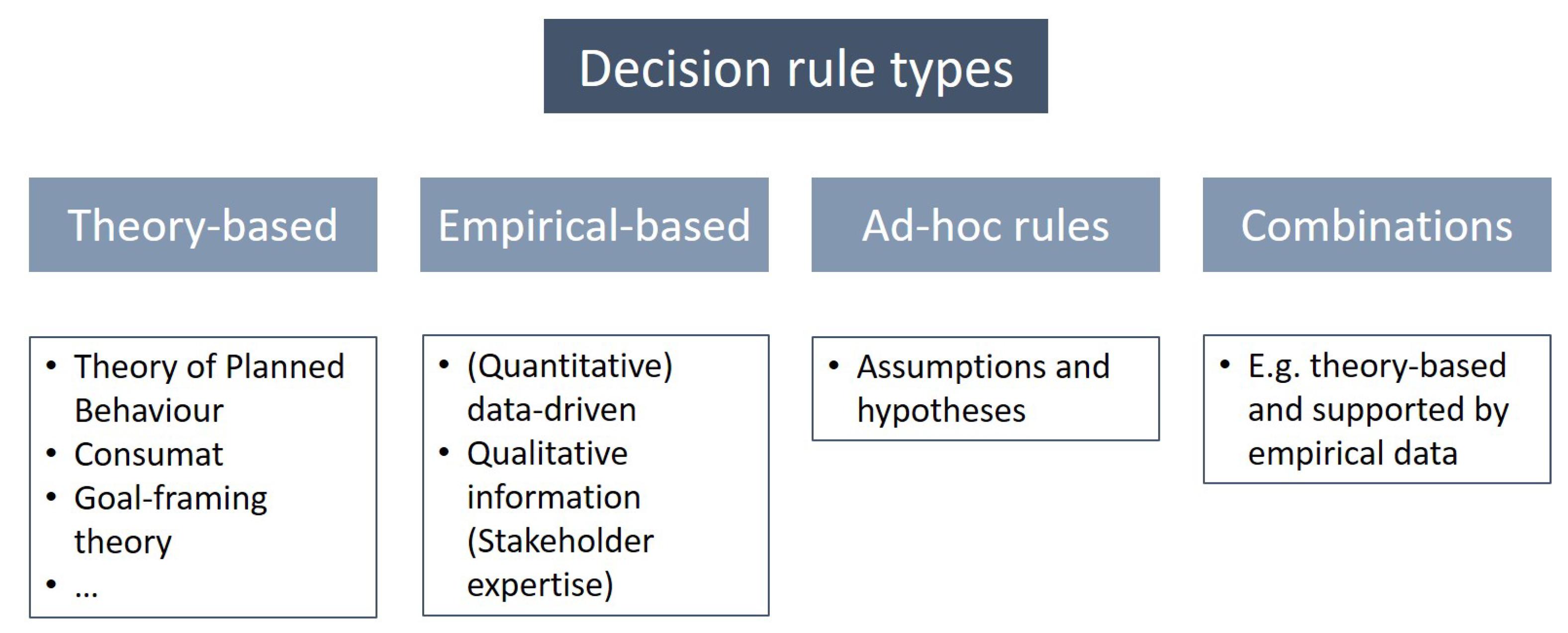
The articles describing the diffusion ABMs are more explicit about the decision-making algorithms. In such models, agents decide to adopt or not adopt (i.e., to invest or not invest in a certain technology or to perform a certain energy-related action) based on specific rules or algorithms. Decision rules range from simple ad-hoc rules to most elaborate models, such as psychosocial or cognitive models [43]. The classification of existing decision models has been previously done by [80] for human agents in ecological ABMs, by [56,57] for agents in ABMs innovation diffusion and by [43] for ABMs of socio-technical systems. The ODD+D by [81] clusters agent decision algorithms based on the nature of the underlying assumptions:
- theory-based (e.g., microeconomic and psychosocial models)
- empirical-based (e.g., statistical regression models, heuristic rules),
- ad-hoc rules (i.e., dummy rules and pure assumptions that are not based on theories or observations),
- combinations of the above methods (see Figure 5).
Most of the diffusion ABMs cited in this article apply theory-based decision models, namely, psychosocial (also called “socio-psychological” or “cognitive”) and microeconomic models. Psychosocial models are based on social psychology theories that assume that human decisions are based on psychological rules, rather than on rational economic rules. The most frequently used psychosocial theory in the selected models is the Theory of Planned Behaviour (TPB) by [82]. It states that human behaviour results from the intention to perform the behaviour; individual attitudes, subjective norms, and perceived expectations can influence the agent to perform such behaviour [83]. Usually, the more favourable these three aspects of human psychology are, the stronger is the person’s intention to perform a certain behaviour [83]. The standard form of TPB is static, i.e., it describes how these three components are translated into intention and action at a given time. The models by [51,66,67] are examples of implementing this theoretical model. Other psychosocial models including “consumat” model by [84] in [68], Norm Activation theory by [85] in [71], the goal-framing theory by [86] in [74], and Influence, Susceptibility, and Conformity Model by [87] in [49], are also used. Several models rely on models from microeconomic or network theories, namely on innovation diffusion models. Azar & Al Ansari [47] draw on the opinion dynamics models by [88,89,90] to represent the effect of energy feedback interventions among building residents.
Another class of frequently used agent decision-making model is the empirical-based heuristic models. They are described as models “not built on any grounded theories” and “having the impression of being ad-hoc” [57]. Agents are often assigned rules derived from empirical data, and also model parameters are selected such that results match simulated output against a real-life observation [57,80]. They might not represent the process of agent decision-making very accurately or realistically, but have the advantage of being easy to implement and to interpret [57]. Heuristic decision rules can be implemented in various ways. Several modellers favour data-driven approaches, thus, implementing machine learning algorithms, such as logistic regression models [59] and artificial neural networks [77]. In this approach, several sets of factors that can affect the adoption of PV or energy-saving behaviour, given that data about those factors are available, are tested. The more qualitative approach is followed by [72,73], who created the decision rules relying on the stakeholder’s expertise.
Some models rely on ad-hoc rules without any validated theory or empirical grounding. Huang et al. [70] derives the agents’ decision logic from relevant secondary literature and assumes that social influence plays a great role in deciding to adopt weatherisation of a dwelling. In this model, agents decide between adopting weatherisation with the Weatherization Assistance Program or without and it depends on several attributes, memory length about the energy costs, current satisfaction level and information level about the assistance program. Mittal et al. [3] developed a decision model similar to [51], but do not apply the TPB. The agents assess the affordability of PV options (i.e., buy, loan, community PV) and the attitudinal factors in the corresponding submodels and make the adoption decision based on certain if-else type rules. The remaining studies are summarised in Table 3.
4.4. Agent Interaction
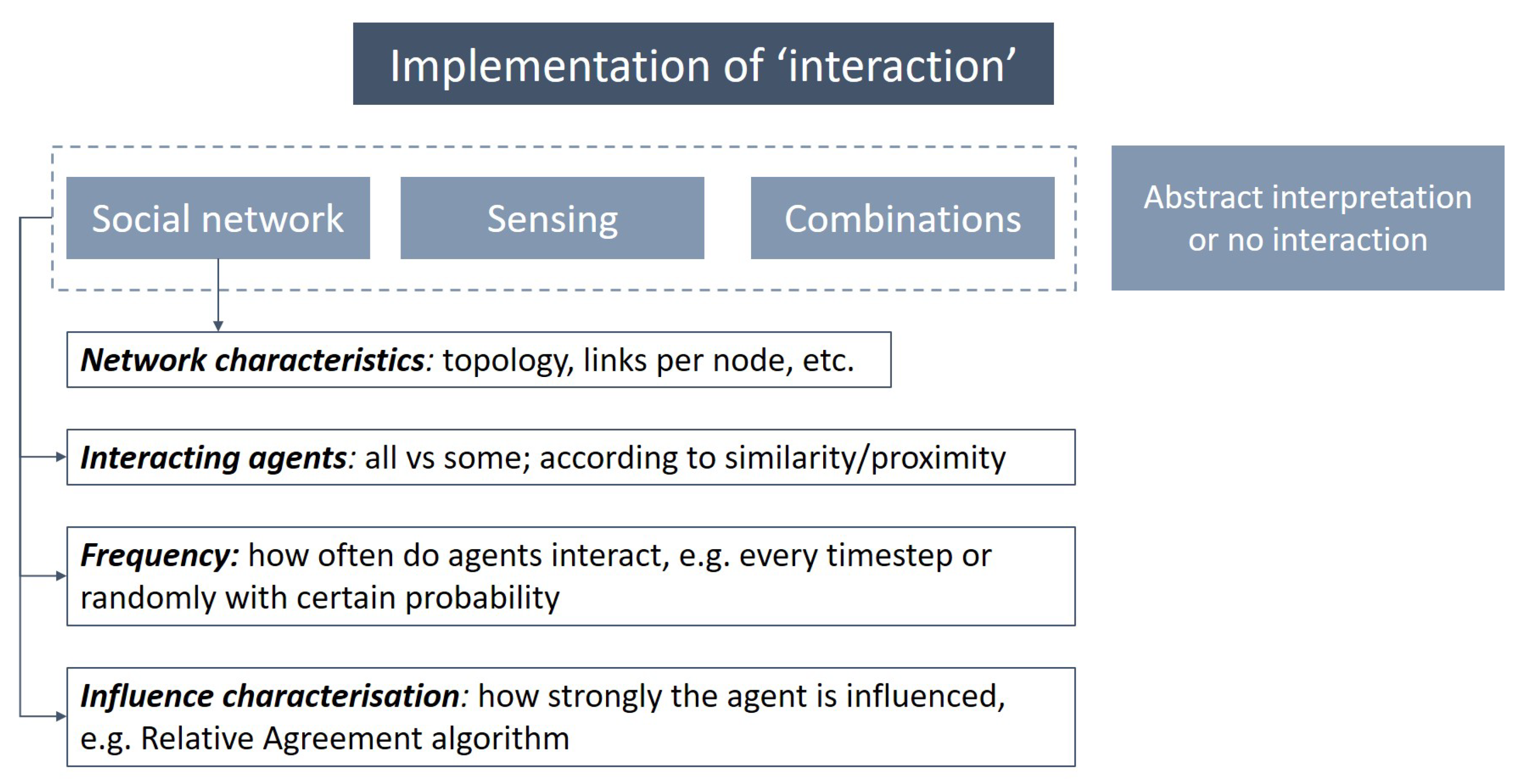
Emergent phenomena to be observed via ABM is the result of not only individual decision-making but also agent interactions [21,78]. The behaviour of agents is often influenced by the information fed from its environment, including other agents. In the ODD the authors differentiate conceptually between ’sensing’ and ’interaction’: the first concept defines what state variables of which other individuals and entities can an agent perceive; the latter is the direct (via communication) or indirect (e.g., via a common resource) interaction between agents or between agents and other entities. However, in practice it is challenging to differentiate between those. For example, human agents’ social influence (also known as ‘peer effect’ or ‘neighbourhood effect’) can be represented using either (or even both) of those concepts, as it seen from the pool of the reviewed papers. Hence, in this work, we consider ‘sensing’ as one of the ways of representing interaction (as depicted in Figure 6).
In the selected studies, one must, first of all, differentiate between studies where agents can interact and influence each other and those where agents do not interact. Only two studies have not considered agent interactions in any way [62,69]. In [73,77], interactions are considered as important, however, treated in an abstract and implicit way. Table 3 shows how interactions are represented in each reviewed study.
The majority of studies which include agent interaction agents are often placed in a network structure, often called “social network”, that imitates the relationship between agents, through which they can exert an influence upon each other based on certain rules (i.e., “peer influence” or “social influence”). The resulting structure allows modelling the social interactions of agents, resulting in the spread of desirable, or non-desirable, ideas, products, or behaviours [91,92] (also called “opinion dynamics”). One common way of doing so is through making an agent’s decision dependent on other agents’ (either selected group of agents or all agents) choice or decisions.
A social network typically consists of two components: individuals or agents (represented by nodes) and social connections (represented by edges or links). It can also have various topologies, e.g., small-world network, and created by various algorithms, e.g., Watts-Strogatz algorithm. Some modellers test the effect of varying the topology and other characteristics (e.g., number of links per node) of social networks [47,48,49]. A modeller should also specify between which agents interaction (or ‘sensing’) occurs, between all agents or certain group of agents or between agents and other entities (e.g., grid cells). In a social network, usually, agents that have a link can interact or the influence of connected agents is more significant compared to those with whom the agent doesn’t have one. This assumption is based on the empirical findings: friends and family have a larger impact on each other’s behaviour than strangers [66,67]. In some cases, agents interact based on similarity (also called ‘homophily’) [3] or geographical proximity [51] (‘neighbour effect’).
Another choice that a modeller should take is regarding the frequency of interactions. Huang et al. [70], for example, let agents that are linked with each other interact every time step, whereas “strangers” (without direct links) interact with a probability of 0.10. The “strength” of the influence can also be characterised in various ways. The most used is the opinion dynamics model by relative agreement algorithm, where agents with similar opinions have a stronger influence on each other than those whose opinions are more polarised [93]. To sum up, there are usually four key things a modeller should consider when characterising an interaction of agents, as we summarise in Figure 6.
4.5. Technologies and Policies Modelled
This subsection discusses the technologies and policies that are in the scope of the reviewed ABMs. Similar to [36], we identify which technologies and policies are explored using ABM. However, since the selected studies are not narrowed down to studies of technology diffusion only, it gives a broader overview of the discussion subject.
4.5.1. Technologies
From the 25 reviewed models, technologies are relevant to 20, while the rest have not modelled technology explicitly. Within these 20 studies, PV system, and specifically, diffusion of PV is the most frequently explored topic, as there are ten studies which focus on that (see Table 2). Majority of these studies consider the diffusion of a single technology: rooftop PV [50,59,60,62,64], feedback device (CO2 meter) [66,67]. In some cases, there could be several options are available for agents: [3,61] let agents choose between buying PV via cash payment of a loan, adopting community solar (i.e., renewable energy community) or opting for green electricity; Ramshani et al. [63] make agents choose the optimal solution for their rooftops—either rooftop PV or green roof; Nava Guerrero et al. [76] introduces the combinations of technologies as “technology state” of a household (i.e., combination of heating system, insulation level, and appliances). Building insulation or renovation is addressed in three studies [69,70,75]. Most studies are interested in the adoption of technologies by households: under what conditions are households willing to adopt these technologies, how does it affect their subsequent energy consumption, etc. Zhang et al. [68] call the latter “learning” and observes how the installation and the subsequent interaction with this technology make them decrease their energy consumption.
Finally, the five studies focus on the energy-related behaviour that is not directly linked to a single technology. For example, the works by [47,48,49,77] investigate how feedback interventions could be improved, so that building occupants consume even less energy. Although the consumption of energy practically occurs as a result of interaction with certain technology (e.g., heater, shower, computer), such details are ignored in these models in order to focus on the macro-level phenomena, such as the interaction of occupants in their network [47]. Similarly, [71] examined the effect of several actions (i.e., investment, conservation, switching) in different socio-political framework conditions without emphasising the technological aspects. For a more detailed description of the review articles regarding ABMs refer to Table A1 (Appendix A).
4.5.2. Policies
The selected 25 works can be the first split into those that explicitly model policy interventions (11) and those that do not (14). The policies covered in the 11 models are of two major types: ones that promote investment for energy-efficient technology (PV, DH, feedback device, etc.) and those that encourage energy-saving behaviour. The examples of the first type of policies are those that stimulate PV system investments [51,60,63,64], assistance programs for weather-proofing [70], and promotional campaigns for feedback devices [67]. The examples of the interventions for stimulating energy-saving are energy feedback mechanisms [47]. Beyond these clusters, Niamir et al. [71] introduces several carbon emission price scenarios to see how it affects the emissions caused by household energy consumption. Busch et al. [73] explore various ways of encouraging different district heating (DH) system developers and found out that creating policy specific to the motivations and capabilities of different actors, enabling networking and learning, and supporting all stages of the decision process is crucial for developing DH network successfully.
The prevailing share of the papers do no implement policies explicitly. They rather explore various socio-economic or other aspects that can affect the policy design or help policymakers make decisions or interpret the results of their model for policy-making [68]. For example, Nava Guerrero et al. [75] investigates the socioeconomic conditions, such as value orientation of the population, gas price changes, the time horizon for investment evaluation, that support the transition to the natural gas-free economy.
The detailed description of how policies are implemented in the models are provided in Table A2 (Appendix B).
4.6. Spatial and Temporal Aspects
Identifying the spatial and temporal scale of the models is important in order to understand the system modelled. Moreover, certain patterns and processes can be dependent on the scale [94] and, thus, they need to be clearly stated. By spatial scale, we mean “geographic scale”, defined as a research area’s spatial extent in a study [94]. The geographic scale of the models considered range from “group of buildings” [47] to an entire city, such as Hamburg [69]. 16 studies describe community, or district, or neighbourhood-scale models, while nine studies are in city-scale [51,67,68,69,73,77]. Although these articles present the models as having been applied to specific geographic scales (i.e., via case studies), it is difficult to say if they can be scaled up or down, as it might depend on many factors.
The chosen scale in ABM usually determines the number of entities (i.e., agents) covered [33]. This can be limited by computers’ processing capacity, especially if decision algorithms are sophisticated, much data is used, or a considered city is very large, e.g., like in [59]. Therefore, the majority of selected models opt for district or neighbourhood scale. Those whose models are in city-scale focus on smaller cities of about 100–150,000 [62,66,67]. Only one model has modelled a city of approx. 174,000 households and the simulation had to be carried out on a supercomputer [51]. There are also such models whose scale depend on the topic of research. For example, DH network development is usually city-scale phenomena [73], the development or properties of energy communities are explored on a neighbourhood or district level [3,72].
Although traditionally ABMs have not focused on the geographic environment and spatial representation, more and more models are striving to represent space explicitly and realistically (e.g., using GIS techniques) [95]. According to [95], models can have three levels of spatial explicitness: (1) implicit and non-geographic representation of space (e.g., social networks that are only partially tied to space); (2) explicitly represented but abstract in how it maps onto reality (e.g., Schelling’s segregation model); (3) explicit and realistic spatial representation. Among the reviewed models, only a few are spatially explicit and realistic. For instance, [51,58,59,64] join building information with actual geographical locations of those buildings and have a clearly defined boundaries of the study area. The rest of the models integrate spatial properties in different, semi-abstract ways. For example, in [3,61] agents in the same community, i.e., neighbours, are defined by a community ID, and each agent in a community becomes aware when somebody in that community installs a PV.
The temporal scale is a duration of a process observed, i.e., time horizon between the start and end of a single simulation run. Temporal resolution represents the unit of a time step in a considered model. According to temporal scale and resolution, the reviewed studies have time horizons of several years and resolutions of 1 month or three month-periods. These models have large simulation horizons and resolutions because the behavioural dynamics captured in those models occur in lower temporal resolutions. For example, in real life, people’s attitudes do not change in a matter of hours. Such time horizons and resolutions are characteristic of policy-guiding models, aiming to observe the effect of a policy intervention over the years. In their models, the authors [51,59] choose the years when adoption data are available, which makes it possible to improve their empirical model in such a way that the simulated outputs fit the real adoption data.
4.7. Empirical Grounding
Empirical grounding of ABMs is becoming more important, especially for models that aim to reflect a specific real-world situation and provide decision support for policymakers and stakeholders [57,96]. As opposed to hypothetical or theoretical (or highly abstract) ABMs, empirical ABMs use real-life data to parameterise models, initialise simulations, and evaluate model validity [57]. Modellers try to improve the realism of agent decision-making algorithms by consulting with system-relevant actors [72,73] or relying on empirical data [59,64,66], e.g., geospatial information on buildings. It is becoming more feasible due to the contemporary trends we observe the availability of high-resolution data sets, the spread of open data culture in science, advances in data analytics, machine learning, and computational power. Therefore, we aim to assess for what purpose, what kind of, and how empirical data is used in the selected ABMs of district energy systems. By empirical data, we mean both qualitative and quantitative data based on observation or experiment.
The review by [36] highlights that empirical data in ABMs are used for two general purposes: (1) to form the agent decision-making algorithm; (2) to determine the specific properties of technologies, policies, etc. that an agent can access to use in their decision rules. In the first case, empirical data from surveys, statistical data (i.e., census), interviews, and other sources are used to determine the attributes (both which attributes and their values) of the agents that are further incorporated in a decision-making framework (as described in Section 4.3). Jensen et al. [66] describe how they utilised empirical data for creating household agents and their social network in the appendix of their article. Building data (i.e., floor area, spatial information, etc.) are connected to agents, and the commercial geo-marketing data defines the “lifestyle” of agents, which further define their affinity for technology and behaviour adoption. Social influence is modelled by introducing a social network based on interviews with households. The second purpose of integrating empirical data involves using statistical data and secondary literature to define other, for example, scenario-relevant information or model parameters (i.e., global parameters). For example, Azar et al. [47] use building energy consumption survey data to initialise the model-level parameter “building energy intensity” and the number of agents in each building. However, it is not easy to determine for all models for what the specific data is used, as authors do not sufficiently describe it. Sometimes the authors refer to another article for detailed information about surveys or stakeholder interviews [73,74].
In general, there are three processes in model building where the use of empirical data make models more reliable and realistic: parametrisation, calibration and validation [37]. The parameterisation is the process of connecting model and target system (i.e., the real system being modelled) via assigning the set of parameters and their values to enable simulation [96]. In line with observations of [37], only a few modellers explicitly differentiate their modelling process into these three phases. Moreover, if calibration and validation are somewhat known to data-driven modellers, the process of parameterisation is not recognised as much. Among the selected models, only [66,67] describe parameterisation in more detail: they select the parameter values to reflect the empirical patterns of ventilation behaviour adoption derived from survey data.
Calibration is the adjustment of parameters to ensure that model output matches the relevant empirical data, e.g., in a specific location and application [37]. The difference to validation is that the parameters are tuned to match a specific context (i.e., location, time), which does not necessarily mean that the model will exhibit accurate results and be predictive upon application in another context. To achieve that it has to be first validated on a separate set of data independent of data used for calibration [57]. The following models describe how they calibrated their models: [62] calibrates the parameters of the logistic function governing the adoption of PV based on the secondary literature and publicly available data; Ramshani et al. [63] performs the partial calibration (i.e., only of the financial submodel) based on the values reported in the literature, experts’ opinions and publicly available datasets; Jensen et al. [66] provides an indirect calibration with three empirical patterns, the same used for parameterisation in [67]. As for the remaining models, some do not differentiate between validation and calibration [60], some call calibration “model fitting” [51], but the majority do not mention calibration at all. Often authors mention the lack of data for calibration as their limitations [63,73].
Validation aims to achieve the matching between the observations of the models and reality. It should not be confused with “verification”, which is the process of making sure the model implementation is carried out correctly with respect to the conceptual model [97]. As ABM is a highly multi-disciplinary and flexible framework, its validation is a highly debated topic. For more detail, we suggest referring to the works of [57,98] that explore this topic in more detail. Our observations are mostly limited to the validation processes provided in the selected works, the majority of which either do not mention validation, state it as a limitation and future task, or have insufficient information on the validation.
Among the models which consider validation, there are two following generic approaches. The first approach is an aggregate behaviour validation, mainly based on statistical data fitting. Rai & Robinson [51] and Lee & Hong [59] applied this way of validation, because they had empirical data on the number of adopters in a given location, over a certain period. Lee & Hong [59] use the Wald test (i.e., Wald Chi-squared test) which tests the significance of a set of independent variables in a statistical model. Rai & Robinson [51] first calibrate the six model parameters by an iterative fitting via historical adoption data and then validate the model in terms of predictive accuracy, i.e., comparing predicted adoption with empirical adoption level for the period starting after the last date in the calibration dataset. Also, they carry out temporal, spatial, and demographic validation [51]. Another group of modellers [47,49,73] pay more attention to the validation of social processes and, by drawing on the work of [99], offer conceptual, operational or structural, and technical validation (by this, [47] refer to verification). Conceptual validation is the process of determining that the theories and assumptions underlying the conceptual model are correct [99] and usually achieved by basing the model on validated concepts [47,49] or the insights from stakeholder workshops [73].
5. Discussion and Conclusions
This article reviews the state-of-the-art ABM approaches in the context of urban energy systems. By analysing a pool of 25 carefully selected research articles, we observe some key domains where ABMs are used to simulate agent decisions and stakeholder behaviours in urban energy systems to guide policy design. The added value of this work is in the deep analysis of the preliminary work in agent-based modelling energy transition of district and neighbourhoods for the purpose of policy testing; understanding the key aspects of ABM foe energy system modelling; and identifying gaps and future research streams.
In the district energy systems domain, the use of ABM for policy implications is becoming more prominent. The ability of ABMs to model complex interactions of independent agents enables the modellers to observe the broader implications of a specific policy design. The model structure, agent types, decision models, spatial and temporal scales are determined by the goals and the questions the ABM seeks to answer. Policy design studies are very versatile when it comes to specific purposes: from evaluating particular measures that stimulate the adoption of technologies, over studying the effect of social connectedness of households, to exploring novel concepts, such as the formation of thermal energy communities. It is important to reiterate that the origin of ABMs was in social and natural sciences. When ABMs become popular in other scientific fields, such as energy systems research, scientists try to adapt the original ABM concepts to fit their specific purposes. Such adaptations are often study-specific, and therefore, some essential modelling details may get lost or unclear to the audience without careful and standardised documentation. In this regard, the ODD protocol provides an essential standardised framework for model documentation.
Our analysis shows tremendous potential in ABMs to help policymakers make better policy decisions, especially in the upcoming years of post-covid recovery. With the Next Generation EU plan that pays a great attention to fair climate transition and funding research that supports such just transition, there’s a chance to accelerate local neighbourhoods’ and districts’ decarbonisation. This is when agent-based models can help a great deal and be used to test various “what-if” scenarios.
The main challenge for future ABM applications in district energy systems is whether the ABM concepts can evolve and scale-up to represent the complexity of agents’ decisions and interactions in a smart and decentralised energy system. Prosumers, i.e., those who self-consume PV energy and sell the surplus contribute vastly to energy transition (especially in countries with higher influx of solar energy) [100]. There are still many gaps and potentials in studying how to encourage the transition of consumers towards prosumers. ABM is useful in this regard, as it can represent different needs and interests of heterogeneous prosumers. That is something that no other modelling paradigm can offer.
Most of the reviewed ABMs deal with the various questions around adopting energy-efficient or renewable energy technology. These adoption decisions represent single-step investment decisions dependent on one decision-maker. However, there is a vast field of opportunity when it comes to exploring phenomena that involve multi-level decision-making and interactions of various stakeholders. Building stock retrofitting and development of district heating system are examples of such phenomena. Though a few exploratory ABMs investigate these topics, there are no models that comprehensively study retrofitting decision-making. The decision-making process and stakeholders will be different depending on whether we are studying social housing [101] or owner-occupied or rental sectors. These differences in decision-making of owner-occupiers, landlords or housing associations, their implications and how to use them to tailor policies should be investigated further too. Furthermore, the studied literature mainly deals with the energy issues of residential neighbourhoods and not commercial or industrial entities. Therefore, we also find it an exciting research avenue to explore whether ABMs, with their unique abilities, can answer some of the challenging energy transition questions related to commercial and industrial stakeholders.
Empirical data can be used to parameterise agent decision-making and provide contextual information to the model. Based on our analysis, we find significant gaps in the use of empirical data. Only a handful of reviewed models have made an explicit effort to clearly describe the use of data for parameterisation, calibration, validation, and verification purposes. Agent and model level parameter selection is often not given the due respect and attention it deserves. As the energy system complexity and, hence, the model complexity increase, careful parameterisation can significantly lower the computational cost. Lastly, careful integration of empirical data for model calibration, validation, and verification purposes significantly improves our confidence in the model and the results for practical purposes.
Author Contributions
Conceptualization, A.A., L.K., F.S. and C.B.H.; methodology, formal analysis, investigation, resources, data curation writing—original draft preparation, A.A.; writing—review and editing, F.S, L.K. and C.B.H.; visualization, A.A.; supervision, L.K. and F.S.; project management, funding acquisition, L.K. All authors have read and agreed to the published version of the manuscript.
Funding
This research has received funding from the European Union’s Horizon 2020 research and innovation programme under the Marie Skłodowska-Curie grant agreement No. 812730.
Institutional Review Board Statement
Not applicable.
Informed Consent Statement
Not applicable.
Data Availability Statement
Not applicable.
Acknowledgments
Special gratitude to Javanshir Fouladvand and Carlo Corinaldesi for fruitful discussions and thoughtful suggestions.
Conflicts of Interest
The authors declare no conflict of interest.
Abbreviations
The following abbreviations are used in this manuscript:
| ABM | Agent-Based Model |
| ABS | Agent-Based Simulation |
| DH | District Heating |
| EC | Energy Champion |
| LD | Linear dichroism |
| EEP | Energy Efficiency Program |
| MAS | Multi-Agent Systems |
| ODD | Overview, Design Concepts and Details |
| ODD+D | Overview, Design Concepts and Details + Decision-making |
| OOP | Object-Oriented Programming |
| PV | Photovoltaic Systems |
| RA | Relative Agreement (algorithm) |
| RE | Renewable Energy |
| SLR | Systematic Literature Review |
| TPB | Theory of Planned Behaviour |
Appendix A. Previous Review Articles

Table A1.
List of previous review articles.
| Study | Focus of the Review | Type of Review | Number of Reviewed Papers | Covered Aspects | Key Conclusions |
|---|---|---|---|---|---|
| [102] | Application of ABM in the built environment domain (building energy and indoor-environmental performance) | selective | 23 | Motivational background, approach for representation of both people (and their behaviour) and environment (e.g., case studies), implementation tools, state of ABM development and its future directions in the domain of buildings’ energy and indoor-environmental performance | Motivation of the studies analyzed: to realistically capture the interactions between occupants as well as the interactions between occupants and their surrounding built environment. |
| [37] | Application of ABM in studying climate-energy policy | selective | 61 | Reasons for using ABM, number and types of markets represented (e.g., transportation, electricity, financial services), empirical basis, time horizon, agent types and numbers, types of bounded rationality, social interactions and networks; link between model features and policy results | 3 main themes identified: focusing on policies that (1) directly trigger emissions reduction, (2) stimulate the diffusion of low-carbon/energy products and technologies, and (3) encourage energy conservation in other ways. Research gaps are identified. |
| [35] | Application of ABM in the built environment domain (building energy and indoor-environmental performance) | systematic | 62 | Thematic analysis from a multi-level perspective of energy transitions; Modelling complexity in energy transitions (complexity categories). | 6 topic areas identified: Electricity Market (25), Consumption Dynamics/ Consumer Behaviour (12), Policy and Planning (9), New Technologies/ Innovation (7), Energy System (6), Transitions (3). Application in Policy and Planning is very important (drives energy transitions). |
| [36] | Adoption of energy efficient technologies by households | systematic | 23 | Technologies studied, barriers to the adoption of energy efficiency, policy measures that are explored using the ABMs, theories used to describe decision making of households and the use of empirical data | Modelled policies: subsidies, regulation and taxation, technology ban, household adoption obligation and various information campaigns. Many of the models are rooted in the TPB, use utility functions, and/or use empirical data. |
| [22] | Application of ABM for understanding technology diffusion of residential energy efficient technologies and to evaluate policies’ effects on adoption. | selective | - | Types of ABM approaches (both theoretical and empirical); applicability and limitations of ABM for modelling of the uptake of en-eff tech-s in energy sector | Key components of ABM for describing the adoption and key decision when intending to model the uptake of energy-efficiency technologies. ABM can model technology diffusion with at least the same accuracy as equation-based modelling when appropriately parameterised based on empirical data, calibrated based on macro-level data, and validated using sensitivity analysis. |
| [17] | ABM work in the area of consumer energy choices, with a focus on the demand side of energy to aid the design of better policies and programmes | selective, critical | about 60 | Limitations of non-ABM approaches, framework for describing the essential features of ABM, use of ABM in practice | Two major types of energy-demand questions that ABM is well-suited to answer: those related to policy design and evaluation, and those related to system design and infrastructure planning. |
| [44] | Application of ABM for analysing smart grids from a systems perspective | selective | 23 | How ABM can be used to analyse electricity systems; typology of agent-based research of electricity systems; review of literature specifically studying smart grids using ABMS techniques is reviewed | ABM is still a limited field of research, but can deliver specific insights about how different agents in a smart grid would interact and which effects would occur on a global level. Valuable input for decision processes of stakeholders and policy making. |
| [45] | Overview of AB electricity market models and present the most relevant work in detail. | selective | 31 | Comparison of current AB electricity models, Methodological questions: Agent learning behavior, Market dynamics and complexity, calibration and validation, Model description and publication. | Choice of specific learning algorithms, more careful and well documented validation and verification procedures as well as the appropriate publication of details of concrete simulation models are crucial for the further development of AB electricity market modeling. |
| [103] | Study of the ABM simulation packages for electricity markets | selective | 4 | Overview of electricity markets, general-purpose ABS tools to introduce some background of ABS, detailed study of four popular ABS packages for Electricity Markets (SEPIA, EMCAS, STEMT-RT, NEMSIM). | ABS packages are divided into 2 types: toolkit (Netlogo, Repast) and software (AnyLogic, AgentSheets) |
Appendix B. Technologies and Policies
Table A2.
Technologies and policy scenarios modelled using ABM.
| Study | Technologies | Decision Regarding Technology | (Policy) Scenarios |
|---|---|---|---|
| [47] | No technology | Energy-saving in buildings | No policy; insights for energy feedback methods, for any building stock |
| [50] | PV | Adoption | No policy |
| [58] | PV | Adoption | Subsidies for low-income and high-income classes; a discount voucher proposed by PV sellers; an information campaigns on environmental issues & on adopting PV |
| [67] | Feedback device (i.e., CO2-meter) | adoption and resulting energy-efficient heating behavior | Promotion-type policies (i.e., marketing strategies) to support product diffusion: giving away, lending out and raising awareness about CO2-meter/feedback device. |
| [66] | Feedback device (i.e., CO2-meter) | adoption and resulting energy-efficient heating behavior | No policy; incentives and financial supports for PV systems are included in economic factors |
| [59] | PV | Adoption | No policy |
| [60] | PV | Adoption | “Self-consumption Communities”: building owners can install PV and sell the electricity to their tenants at prices lower than the retail price of electricity |
| [3] | PV | Adoption | No policy; different renewable energy models (e.g., solar community, buy/lease PV, etc) with different conditions (price, time, etc) for agents to adopt |
| [61] | PV | Adoption | No policy; different renewable energy models (e.g., solar community, buy/lease PV, etc) with different conditions (price, time, etc) for agents to adopt |
| [62] | PV | Adoption | No policy |
| [71] | PV | Adoption | Carbon price as a climate policy scenario |
| [51] | PV | Adoption | Rebates for low-income households (i.e., households in the bottom quartile of wealth, proxied by home value). |
| [63] | PV, green roof | Adoption | Investment Tax Credit, promotional campaigns |
| [64] | PV | Adoption | Self-consumption scheme (PV electricity is sold at market price) and Citizen/Renewable Energy Community scheme (share the electricity produced by a single PV unit with many citizens, e.g., in a condominium) |
| [68] | Smart meter | learning after SM adoption, energy-saving behaviour | No policy; insights for facilitation of learning following the smart meter roll-out |
| [73] | DH network | project development | Forcing the Local Authorities to have a heat strategy; increasing the availability of capital finance for all DH project instigators; support community instigators, i.e., include proactive LA (Energy Leader) and support at every stage of the DH development |
| [72] | Renewable heating technology | joining or exiting a thermal energy community | No policy |
| [74] | Electric appliances, insulation | purchase | No policy described, but the model is capable |
| [70] | Weather-proofing (“weatherization” for winter) technology | Adoption | Publicly funded Weatherization Assistance Programs that are intended to help low-resource residents improve the energy efficiency of their homes |
| [75] | Insulation, renewable heating | investments in new technology | No policy; changes in natural gas price and electricity price are taken as proxies for market forces and policies |
| [76] | insulation, renewable heating | investments in new technology | Fiscal policy (i.e., linear growth of natural gas taxes, taxes on electricity, and regulated price of heat from networks) and disconnection from gas network. |
| [69] | Renovation technology | renovation decision | No policy |
| [77] | No technology | energy-saving behaviour | Range of external situational factors are tested: social norms related to energy saving, popularization of economic energy-saving policies, etc. |
| [48] | No technology | energy-saving behaviour | No policy; insights for EEP |
| [49] | No technology | energy-saving behaviour | No policy; insights for normative interventions (ecofeedback programs) |
References
- Global Alliance for Buildings and Construction, International Energy Agency and the United Nations Environment Programme. 2019 Global Status Report for Buildings and Construction. Available online: https://www.unep.org/resources/publication/2019-global-status-report-buildings-and-construction-sector (accessed on 28 November 2021).
- Nematchoua, M.K.; Sadeghi, M.; Reiter, S. Strategies and scenarios to reduce energy consumption and CO2 emission in the urban, rural and sustainable neighbourhoods. Sustain. Cities Soc. 2021, 72, 103053. [Google Scholar] [CrossRef]
- Mittal, A.; Krejci, C.; Dorneich, M.; Fickes, D. An agent-based approach to modeling zero energy communities. Sol. Energy 2019, 191, 193–204. [Google Scholar] [CrossRef]
- Marique, A.F.; Reiter, S. A simplified framework to assess the feasibility of zero-energy at the neighbourhood/community scale. Energy Build. 2014, 82, 114–122. [Google Scholar] [CrossRef] [Green Version]
- Marszal, A.J.; Heiselberg, P.; Bourrelle, J.S.; Musall, E.; Voss, K.; Sartori, I.; Napolitano, A. Zero Energy Building—A review of definitions and calculation methodologies. Energy Build. 2011, 43, 971–979. [Google Scholar] [CrossRef]
- Paiho, S.; Ketomäki, J.; Kannari, L.; Häkkinen, T.; Shemeikka, J. A new procedure for assessing the energy-efficient refurbishment of buildings on district scale. Sustain. Cities Soc. 2019, 46, 101454. [Google Scholar] [CrossRef]
- Rose, J.; Thomsen, K.E.; Domingo-Irigoyen, S.; Bolliger, R.; Venus, D.; Konstantinou, T.; Mlecnik, E.; Almeida, M.; Barbosa, R.; Terés-Zubiaga, J.; et al. Building renovation at district level–Lessons learned from international case studies. Sustain. Cities Soc. 2021, 72, 103037. [Google Scholar] [CrossRef]
- Saheb, Y.; Shnapp, S.; Paci, D. From Nearly-Zero Energy Buildings to Net-Zero Energy Districts—Lessons Learned from Existing EU Projects, EUR 29734 EN; Publications Office of the European Union: Luxembourg, 2019. [Google Scholar] [CrossRef]
- Schneider, S.; Bartlmä, N.; Leibold, J.; Schöfmann, P.; Tabakovic, M.; Zelger, T. New Assessment Method for Buildings and Districts towards “Net Zero Energy Buildings” Compatible with the Energy Scenario 2050. In Proceedings of the REAL CORP 2019: IS THIS THE REAL WORLD? Perfect Smart Cities vs. Real Emotional Cities, Karlsruhe, Germany, 2–4 April 2019; pp. 511–520. [Google Scholar]
- Brozovsky, J.; Gustavsen, A.; Gaitani, N. Zero emission neighbourhoods and positive energy districts—A state-of-the-art review. Sustain. Cities Soc. 2021, 72, 103013. [Google Scholar] [CrossRef]
- Schöfmann, P.; Zelger, T.; Bartlmä, N.; Schneider, S.; Leibold, J.; Bell, D. Zukunftsquartier. Weg zum Plus-Energie-Quartier in Wien. Available online: https://nachhaltigwirtschaften.at/resources/sdz_pdf/schriftenreihe-2020-11-zukunftsquartier.pdf (accessed on 28 November 2021).
- Geschäftsstelle Schweiz Hauptstadtregion. Konzept. Eckpunkte von Plusenergie-Quartieren. 2020. Available online: https://plusenergiequartier.ch/konzept/ (accessed on 29 November 2021).
- JPI Urban Europe/SET Plan Action 3.2. White Paper on PED Reference Framework for Positive Energy Districts and Neighbourhoods. 2020. Available online: https://jpi-urbaneurope.eu/app/uploads/2020/04/White-Paper-PED-Framework-Definition-2020323-final.pdf (accessed on 30 November 2021).
- Derkenbaeva, E.; Halleck Vega, S.; Hofstede, G.J.; van Leeuwen, E. Positive energy districts: Mainstreaming energy transition in urban areas. Renew. Sustain. Energy Rev. 2022, 153, 111782. [Google Scholar] [CrossRef]
- Bruck, A.; Ruano, S.D.; Auer, H. A Critical Perspective on Positive Energy Districts in Climatically Favoured Regions: An Open-Source Modelling Approach Disclosing Implications and Possibilities. Energies 2021, 14, 4864. [Google Scholar] [CrossRef]
- Klein, M.; Frey, U.J.; Reeg, M. Models within models—Agent-based modelling and simulation in energy systems analysis. J. Artif. Soc. Soc. Simul. 2019, 22, 6. [Google Scholar] [CrossRef]
- Rai, V.; Henry, A.D. Agent-based modelling of consumer energy choices. Nat. Clim. Chang. 2016, 6, 556–562. [Google Scholar] [CrossRef]
- Chang, M.; Thellufsen, J.Z.; Zakeri, B.; Pickering, B.; Pfenninger, S.; Lund, H.; Østergaard, P.A. Trends in tools and approaches for modelling the energy transition. Appl. Energy 2021, 290, 116731. [Google Scholar] [CrossRef]
- Després, J.; Hadjsaid, N.; Criqui, P.; Noirot, I. Modelling the impacts of variable renewable sources on the power sector: Reconsidering the typology of energy modelling tools. Energy 2015, 80, 486–495. [Google Scholar] [CrossRef]
- Ringkjøb, H.K.; Haugan, P.M.; Solbrekke, I.M. A review of modelling tools for energy and electricity systems with large shares of variable renewables. Renew. Sustain. Energy Rev. 2018, 96, 440–459. [Google Scholar] [CrossRef]
- Bonabeau, E. Agent-based modeling: Methods and techniques for simulating human systems. Proc. Natl. Acad. Sci. USA 2002, 99, 7280–7287. [Google Scholar] [CrossRef] [PubMed] [Green Version]
- Moglia, M.; Cook, S.; McGregor, J. A review of Agent-Based Modelling of technology diffusion with special reference to residential energy efficiency. Sustain. Cities Soc. 2017, 31, 173–182. [Google Scholar] [CrossRef]
- Allwood, J.M.; Bosetti, V.; Dubash, N.K.; D’Agosto, M.; Brazil, A.; Baiocchi, G.; Barrett, J.; Broome, J.; Brunner, S.; Olvera, M.C.; et al. Glossary, Acronyms and Chemical Symbols. In Climate Change 2014: Mitigation of Climate Change. Contribution of Working Group III to the Fifth Assessment Report of the Intergovernmental Panel on Climate Change; Technical Report; Cambridge University Press: Cambridge, UK; New York, NY, USA, 2014; Available online: https://www.ipcc.ch/site/assets/uploads/2018/02/ipcc_wg3_ar5_annex-i.pdf (accessed on 30 November 2021).
- Keirstead, J.; Jennings, M.; Sivakumar, A. A review of urban energy system models: Approaches, challenges and opportunities. Renew. Sustain. Energy Rev. 2012, 16, 3847–3866. [Google Scholar] [CrossRef] [Green Version]
- Eurostat. Glossary: Degree of Urbanisation—Statistics Explained. Available online: https://ec.europa.eu/eurostat/statistics-explained/index.php?title=Glossary:Degree_of_urbanisation (accessed on 28 November 2021).
- Bottecchia, L.; Lubello, P.; Zambelli, P.; Carcasci, C.; Kranzl, L. The potential of simulating energy systems: The multi energy systems simulator model. Energies 2021, 14, 5724. [Google Scholar] [CrossRef]
- Dincer, I.; Rosen, M.A. Exergy Analysis of Cogeneration and District Energy Systems. In Exergy; Elsevier: Amsterdam, The Netherlands, 2013; pp. 285–302. [Google Scholar] [CrossRef]
- Dragoon, K. DM for Integrating Variable Renewable Energy: A Northwest Perspective. In Renewable Energy Integration: Practical Management of Variability, Uncertainty, and Flexibility in Power Grids, 2nd ed.; Elsevier: Amsterdam, The Netherlands, 2017; pp. 245–259. [Google Scholar] [CrossRef]
- Lake, A.; Rezaie, B.; Beyerlein, S. Review of district heating and cooling systems for a sustainable future. Renew. Sustain. Energy Rev. 2017, 67, 417–425. [Google Scholar] [CrossRef]
- Nageler, P.; Heimrath, R.; Mach, T.; Hochenauer, C. Prototype of a simulation framework for georeferenced large-scale dynamic simulations of district energy systems. Appl. Energy 2019, 252, 113469. [Google Scholar] [CrossRef]
- Allegrini, J.; Orehounig, K.; Mavromatidis, G.; Ruesch, F.; Dorer, V.; Evins, R. A review of modelling approaches and tools for the simulation of district-scale energy systems. Renew. Sustain. Energy Rev. 2015, 52, 1391–1404. [Google Scholar] [CrossRef]
- Huang, P.; Copertaro, B.; Zhang, X.; Shen, J.; Löfgren, I.; Rönnelid, M.; Fahlen, J.; Andersson, D.; Svanfeldt, M. A review of data centers as prosumers in district energy systems: Renewable energy integration and waste heat reuse for district heating. Appl. Energy 2020, 258, 114109. [Google Scholar] [CrossRef]
- Mahmoud, M.; Ramadan, M.; Naher, S.; Pullen, K.; Baroutaji, A.; Olabi, A.G. Recent advances in district energy systems: A review. Therm. Sci. Eng. Prog. 2020, 20, 100678. [Google Scholar] [CrossRef]
- Schweiger, G.; Heimrath, R.; Falay, B.; O’Donovan, K.; Nageler, P.; Pertschy, R.; Engel, G.; Streicher, W.; Leusbrock, I. District energy systems: Modelling paradigms and general-purpose tools. Energy 2018, 164, 1326–1340. [Google Scholar] [CrossRef]
- Hansen, P.; Liu, X.; Morrison, G.M. Agent-based modelling and socio-technical energy transitions: A systematic literature review. Energy Res. Soc. Sci. 2019, 49, 41–52. [Google Scholar] [CrossRef]
- Hesselink, L.X.; Chappin, E.J. Adoption of energy efficient technologies by households – Barriers, policies and agent-based modelling studies. Renew. Sustain. Energy Rev. 2019, 99, 29–41. [Google Scholar] [CrossRef]
- Castro, J.; Drews, S.; Exadaktylos, F.; Foramitti, J. A review of agent-based modeling of climate-energy policy. WIREs Clim Chang. 2020, 11, e647. [Google Scholar] [CrossRef] [Green Version]
- Wooldridge, M.J.; Wooldridge, M.J. The Logical Modelling of Computational Multi-Agent Systems 1992. Available online: http://citeseerx.ist.psu.edu/viewdoc/summary?doi=10.1.1.34.6293 (accessed on 28 November 2021).
- Lez-Briones, A.; De La Prieta, F.; Mohamad, M.; Omatu, S.; Corchado, J. Multi-agent systems applications in energy optimization problems: A state-of-the-art review. Energies 2018, 11, 1928. [Google Scholar] [CrossRef] [Green Version]
- Mahmood, D.; Javaid, N.; Ahmed, I.; Alrajeh, N.; Niaz, I.A.; Khan, Z.A. Multi-agent-based sharing power economy for a smart community. Int. J. Energy Res. 2017, 41, 2074–2090. [Google Scholar] [CrossRef]
- Tomicic, I.; Schatten, M. A case study on renewable energy management in an eco-village community in Croatia—An agent based approach. Int. J. Ren. Energy Res. 2016, 6, 1307–1317. [Google Scholar]
- Yasir, M.; Purvis, M.M.; Purvis, M.M.; Savarimuthu, B.B.T.R.B. Complementary-based coalition formation for energy microgrids. Comput. Intell. 2018, 34, 679–712. [Google Scholar] [CrossRef]
- van Dam, K.H.; Nikolic, I.; Lukszo, Z. Agent-Based Modelling of Socio-Technical Systems; Springer Science+Business Media: Dordrecht, The Netherlands, 2013. [Google Scholar] [CrossRef]
- Ringler, P.; Keles, D.; Fichtner, W. Agent-based modelling and simulation of smart electricity grids and markets—A literature review. Renew. Sustain. Energy Rev. 2016, 57, 205–215. [Google Scholar] [CrossRef]
- Weidlich, A.; Veit, D. A critical survey of agent-based wholesale electricity market models. Energy Econ. 2008, 30, 1728–1759. [Google Scholar] [CrossRef]
- Azar, E.; Nikolopoulou, C.; Papadopoulos, S. Integrating and optimizing metrics of sustainable building performance using human-focused agent-based modeling. Appl. Energy 2016, 183, 926–937. [Google Scholar] [CrossRef]
- Azar, E.; Al Ansari, H. Multilayer Agent-Based Modeling and Social Network Framework to Evaluate Energy Feedback Methods for Groups of Buildings. J. Comput. Civ. Eng. 2017, 31, 04017007. [Google Scholar] [CrossRef]
- Zarei, M.; Maghrebi, M. Targeted selection of participants for energy efficiency programs using genetic agent-based (GAB) framework. Energy Effic. 2020, 13, 823–833. [Google Scholar] [CrossRef]
- Zarei, M.; Maghrebi, M. Improving Efficiency of Normative Interventions by Characteristic-Based Selection of Households: An Agent-Based Approach. J. Comput. Civ. Eng. 2020, 34, 04019042. [Google Scholar] [CrossRef]
- Boumaiza, A.; Abbar, S.; Mohandes, N.; Sanfilippo, A. Modeling the impact of innovation diffusion on solar PV adoption in city neighborhoods. Int. J. Renew. Energy Res. 2018, 8, 1749–1762. [Google Scholar]
- Rai, V.; Robinson, S.A. Agent-based modeling of energy technology adoption: Empirical integration of social, behavioral, economic, and environmental factors. Environ. Model. Softw. 2015, 70, 163–177. [Google Scholar] [CrossRef] [Green Version]
- Grimm, V.; Berger, U.; Bastiansen, F.; Eliassen, S.; Ginot, V.; Giske, J.; Goss-Custard, J.; Grand, T.; Heinz, S.K.; Huse, G.; et al. A standard protocol for describing individual-based and agent-based models. Ecol. Model. 2006, 198, 115–126. [Google Scholar] [CrossRef]
- Grimm, V.; Berger, U.; DeAngelis, D.L.; Polhill, J.G.; Giske, J.; Railsback, S.F. The ODD protocol: A review and first update. Ecol. Model. 2010, 221, 2760–2768. [Google Scholar] [CrossRef] [Green Version]
- Grimm, V.; Railsback, S.F.; Vincenot, C.E.; Berger, U.; Gallagher, C.; Deangelis, D.L.; Edmonds, B.; Ge, J.; Giske, J.; Groeneveld, J.; et al. The ODD protocol for describing agent-based and other simulation models: A second update to improve clarity, replication, and structural realism. J. Artif. Soc. Soc. Simul. 2020, 23, 7. [Google Scholar] [CrossRef] [Green Version]
- Starfield, A.M.; Smith, K.A.; Bleloch, A.L. How to Model It: Problem Solving for the Computer Age; McGraw Hill: New York, NY, USA, 1990. [Google Scholar]
- Kiesling, E.; Günther, M.; Stummer, C.; Wakolbinger, L.M. Agent-based simulation of innovation diffusion: A review. Cent. Eur. J. Oper. Res. 2012, 20, 183–230. [Google Scholar] [CrossRef]
- Zhang, H.; Vorobeychik, Y. Empirically grounded agent-based models of innovation diffusion: A critical review. Artif. Intell. Rev. 2019, 52, 707–741. [Google Scholar] [CrossRef] [Green Version]
- Caprioli, C.; Bottero, M.; De Angelis, E. Supporting policy design for the diffusion of cleaner technologies: A spatial empirical agent-based model. ISPRS Int. J. Geo-Inf. 2020, 9, 581. [Google Scholar] [CrossRef]
- Lee, M.; Hong, T. Hybrid agent-based modeling of rooftop solar photovoltaic adoption by integrating the geographic information system and data mining technique. Energy Convers. Manag. 2019, 183, 266–279. [Google Scholar] [CrossRef]
- Mehta, P.; Griego, D.; Nunez-Jimenez, A.; Schlueter, A. The Impact of self-consumption regulation on individual and community solar PV adoption in Switzerland: An agent-based model. J. Phys. Conf. Ser. 2019, 1343, 012143. [Google Scholar] [CrossRef]
- Mittal, A.; Krejci, C.C.; Dorneich, M.C. An agent-based approach to designing residential renewable energy systems. Renew. Sustain. Energy Rev. 2019, 112, 1008–1020. [Google Scholar] [CrossRef]
- Muaafa, M.; Adjali, I.; Bean, P.; Fuentes, R.; Kimbrough, S.O.; Murphy, F.H. Can adoption of rooftop solar panels trigger a utility death spiral? A tale of two U.S. cities. Energy Res. Soc. Sci. 2017, 34, 154–162. [Google Scholar] [CrossRef]
- Ramshani, M.; Li, X.; Khojandi, A.; Omitaomu, O. An agent-based approach to study the diffusion rate and the effect of policies on joint placement of photovoltaic panels and green roof under climate change uncertainty. Appl. Energy 2020, 261, 114402. [Google Scholar] [CrossRef]
- Schiera, D.S.; Minuto, F.D.; Bottaccioli, L.; Borchiellini, R.; Lanzini, A. Analysis of Rooftop Photovoltaics Diffusion in Energy Community Buildings by a Novel GIS- and Agent-Based Modeling Co-Simulation Platform. IEEE Access 2019, 7, 93404–93432. [Google Scholar] [CrossRef]
- Strang, D.; Soule, S.A. Diffusion in organizations and social movements: From Hybrid Corn to Poison Pills. Annu. Rev. Sociol. 1998, 24, 265–290. [Google Scholar] [CrossRef]
- Jensen, T.; Holtz, G.; Baedeker, C.; Chappin, É.J.L. Energy-efficiency impacts of an air-quality feedback device in residential buildings: An agent-based modeling assessment. Energy Build. 2016, 116, 151–163. [Google Scholar] [CrossRef] [Green Version]
- Jensen, T.; Chappin, É. Reducing domestic heating demand: Managing the impact of behavior-changing feedback devices via marketing. J. Environ. Manag. 2017, 197, 642–655. [Google Scholar] [CrossRef] [Green Version]
- Zhang, T.; Siebers, P.O.; Aickelin, U. Simulating user learning in authoritative technology adoption: An agent based model for council-led smart meter deployment planning in the UK. Technol. Forecast. Soc. Chang. 2016, 106, 74–84. [Google Scholar] [CrossRef]
- Preisler, T.; Dethlefs, T.; Renz, W.; Dochev, I.; Seller, H.; Peters, I. Towards an agent-based simulation of building stock development for the city of hamburg. In Proceedings of the 2017 Federated Conference on Computer Science and Information Systems, FedCSIS 2017, Prague, Czech Republic, 3–6 September 2017; pp. 317–326. [Google Scholar] [CrossRef]
- Huang, W.; Krejci, C.C.; Dorneich, M.C.; Passe, U.; Shenk, L.; Stonewall, J. Analyzing residential weatherization decisions using hybrid simulation modeling. Build. Simul. 2019, 12, 517–534. [Google Scholar] [CrossRef]
- Niamir, L.; Kiesewetter, G.; Wagner, F.; Schöpp, W.; Filatova, T.; Voinov, A.; Bressers, H. Assessing the macroeconomic impacts of individual behavioral changes on carbon emissions. Clim. Chang. 2020, 158, 141–160. [Google Scholar] [CrossRef] [Green Version]
- Fouladvand, J.; Mouter, N.; Ghorbani, A.; Herder, P. Formation and continuation of thermal energy community systems: An explorative agent-based model for the netherlands. Energies 2020, 13, 2829. [Google Scholar] [CrossRef]
- Busch, J.; Roelich, K.; Bale, C.S.E.; Knoeri, C. Scaling up local energy infrastructure; An agent-based model of the emergence of district heating networks. Energy Policy 2017, 100, 170–180. [Google Scholar] [CrossRef] [Green Version]
- Gotts, N.M.; Polhill, G. Experiments with a model of domestic energy demand. J. Artif. Soc. Soc. Simul. 2017, 20, 11. [Google Scholar] [CrossRef] [Green Version]
- Nava Guerrero, G.D.C.; Korevaar, G.; Hansen, H.H.; Lukszo, Z. Agent-based modeling of a thermal energy transition in the built environment. Energies 2019, 12, 856. [Google Scholar] [CrossRef] [Green Version]
- Nava-Guerrero, G.D.C.G.d.C.; Hansen, H.H.H.; Korevaar, G.; Lukszo, Z. The effect of group decisions in heat transitions: An agent-based approach. Energy Policy 2021, 156, 112306. [Google Scholar] [CrossRef]
- Yue, T.; Long, R.; Chen, H.; Liu, J.; Liu, H.; Gu, Y. Energy-saving behavior of urban residents in China: A multi-agent simulation. J. Clean. Prod. 2020, 252, 119623. [Google Scholar] [CrossRef]
- Macal, C.M.; North, M.J. Tutorial on agent-based modelling and simulation. J. Simul. 2010, 4, 151–162. [Google Scholar] [CrossRef]
- Jennings, N.R. On agent-based software engineering. Artif. Intell. 2000, 117, 277–296. [Google Scholar] [CrossRef] [Green Version]
- An, L. Modeling human decisions in coupled human and natural systems: Review of agent-based models. Ecol. Model. 2012, 229, 25–36. [Google Scholar] [CrossRef]
- Müller, B.; Bohn, F.; Dreßler, G.; Groeneveld, J.; Klassert, C.; Martin, R.; Schlüter, M.; Schulze, J.; Weise, H.; Schwarz, N. Describing human decisions in agent-based models—ODD+D, an extension of the ODD protocol. Environ. Model. Softw. 2013, 48, 37–48. [Google Scholar] [CrossRef]
- Ajzen, I. The theory of planned behavior. Organ. Behav. Hum. Decis. Process. 1991, 50, 179–211. [Google Scholar] [CrossRef]
- Ajzen, I. Perceived Behavioral Control, Self-Efficacy, Locus of Control, and the Theory of Planned Behavior. J. Appl. Soc. Psychol. 2002, 32, 665–683. [Google Scholar] [CrossRef]
- Jager, W. Modelling Consumer Behaviour. Ph.D. Thesis, University of Groningen, Gronigen, The Netherlands, 2000; p. 240. [Google Scholar]
- Onwezen, M.C.; Antonides, G.; Bartels, J. The Norm Activation Model: An exploration of the functions of anticipated pride and guilt in pro-environmental behaviour. J. Econ. Psychol. 2013, 39, 141–153. [Google Scholar] [CrossRef]
- Lindenberg, S.; Steg, L. Normative, Gain and Hedonic Goal Frames Guiding Environmental Behavior. J. Soc. Issues 2007, 63, 117–137. [Google Scholar] [CrossRef] [Green Version]
- Duggins, P. A psychologically-motivated model of opinion change with applications to american politics. arXiv 2014, arXiv:1406.7770. [Google Scholar] [CrossRef]
- Deffuant, G.; Neau, D.; Amblard, F.; Weisbuch, G. Mixing beliefs among interacting agents. Adv. Complex Syst. 2000, 3, 87–98. [Google Scholar] [CrossRef]
- Hegselmann, R.; Krause, U. Opinion dynamics and bounded confidence models, analysis and simulation. J. Artif. Soc. Soc. Simul. 2002, 5, 1–24. Available online: https://www.jasss.org/5/3/2/2.pdf (accessed on 28 November 2021).
- Mobilia, M.; Petersen, A.; Redner, S. On the role of zealotry in the voter model. J. Stat. Mech. Theory Exp. 2007, 2007, P08029. [Google Scholar] [CrossRef]
- Mason, M.F.; Norton, M.I.; Van Horn, J.D.; Wegner, D.M.; Grafton, S.T.; Macrae, C.N. Wandering minds: The default network and stimulus-independent thought. Science 2007, 315, 393–395. [Google Scholar] [CrossRef] [PubMed] [Green Version]
- Newman, M.E. The structure and function of complex networks. Siam Rev. 2003, 45, 167–256. [Google Scholar] [CrossRef] [Green Version]
- Deffuant, G.; Amblard, F.; Weisbuch, G.; Faure, T. How can extremism prevail? A study based on the relative agreement interaction model. J. Artif. Soc. Soc. Simul. 2002, 5, 27. [Google Scholar]
- Dabiri, Z.; Blaschke, T. Scale matters: A survey of the concepts of scale used in spatial disciplines. Eur. J. Remote Sens. 2019, 52, 419–435. [Google Scholar] [CrossRef] [Green Version]
- Manson, S.; An, L.; Clarke, K.C.; Heppenstall, A.; Koch, J.; Krzyzanowski, B.; Morgan, F.; O’sullivan, D.; Runck, B.C.; Shook, E.; et al. Methodological issues of spatial agent-based models. J. Artif. Soc. Soc. Simul. 2020, 23. [Google Scholar] [CrossRef]
- Smajgl, A.; Barreteau, O. Empirical Agent-Based Modelling—Challenges and Solutions. Volume 1, The Characterisation and Parameterisation of Empirical Agent-Based Models; Springer Science+Business Media: New York, NY, USA, 2014; Chapter 1. [Google Scholar]
- Carson, J. Verification and validation. In Estimating Impact: A Handbook of Computational Methods and Models for Anticipating Economic, Social, Political and Security Effects in International Interventions; Springer: Boston, MA, USA, 2010; pp. 311–336. [Google Scholar] [CrossRef]
- Fagiolo, G.; Birchenhall, C.; Windrum, P. Empirical validation in agent-based models: Introduction to the special issue. Comput. Econ. 2007, 30, 189–194. [Google Scholar] [CrossRef]
- Yilmaz, L. Validation and verification of social processes within agent-based computational organization models. Comput. Math. Organ. Theory 2006, 12, 283–312. [Google Scholar] [CrossRef]
- Colasante, A.; D’Adamo, I.; Morone, P. What drives the solar energy transition? The effect of policies, incentives and behavior in a cross-country comparison. Energy Res. Soc. Sci. 2022, 85, 102405. [Google Scholar] [CrossRef]
- Oliveira, R.; Almeida, R.M.; Figueiredo, A.; Vicente, R. A Case Study on a Stochastic-Based Optimisation Approach towards the Integration of Photovoltaic Panels in Multi-Residential Social Housing. Energies 2021, 14, 7615. [Google Scholar] [CrossRef]
- Berger, C.; Mahdavi, A. Review of current trends in agent-based modeling of building occupants for energy and indoor-environmental performance analysis. Build. Environ. 2020, 173, 106726. [Google Scholar] [CrossRef]
- Zhou, Z.; Chan, W.K.; Chow, J.H. Agent-based simulation of electricity markets: A survey of tools. Artif. Intell. Rev. 2007, 28, 305–342. [Google Scholar] [CrossRef]
Figure 1.
Representative application field of Multi-Agent Systems (based on [44]).
Figure 1.
Representative application field of Multi-Agent Systems (based on [44]).

Figure 2.
PRISMA Flow Diagram of study selection for reviewing ABM of urban district energy systems.
Figure 2.
PRISMA Flow Diagram of study selection for reviewing ABM of urban district energy systems.

Figure 3.
Two major thematic clusters based on model purposes within the ABM of urban district energy systems.
Figure 3.
Two major thematic clusters based on model purposes within the ABM of urban district energy systems.

Figure 4.
Agents in the reviewed models.

Figure 5.
Types of decision-making frameworks.

Figure 6.
Ways of implementing ’interactions’ and relevant modelling choices.

Table 1.
Model purposes and model outputs of the selected studies—Diffusion ABMs.
| Study | Model Purpose | Model Output |
|---|---|---|
| [47] | Explore the effect of social-network characteristics on the diffusion process of energy conservation | % energy savings from different feedback methods with various social network characteristics |
| [50] | Examine the impact of information diffusion algorithm on residential PV adoption in city neighbourhoods | Number of new and total adopters over time |
| [58] | Test alternative policy scenarios for PV adoption in a neighbourhood | Number of PV adoptions per year (simulated vs. real data), spatial visualisation of total adoptions |
| [67] | Design and test marketing strategies for feedback devices (CO2-meter) to identify which would be most effective | Technology and shock ventilation behaviour adoption for different lifestyles |
| [66] | Identify the effect of the ‘CO2 meter’ (feedback device) on energy-efficient heating behaviour | Adoption numbers with various marketing strategies (awareness, give-away device, training) and their locations |
| [59] | Analyse diffusion patterns of rooftop PV under the influence of five factors on the adoption | Number of adopters over time; spatial representation of adoption |
| [60] | Explore individual and community solar PV adoption under the Energy Act in Switzerland | Installed capacity of individual and community PV systems over time |
| [3] | Test consumer adoption behaviours over time in the presence of different renewable energy options | Number of adopters by renewable options, restricted households, % of neighbourhood RE |
| [61] | Predict the consumer adoption of different renewable energy models and to determine the resulting impacts on energy system performance | Utility and solar installer revenues, total power added to the grid, total number of adopters, number of rooftop PV and community solar adopters over time |
| [62] | Determine the effect of PV diffusion on the profitability of utilities | % of buildings with installed PV, % of new installations per year, % of demand met by PV, spatial representation of building adoption. |
| [71] | Observe the impact of socioeconomic heterogeneity, social dynamics, and carbon pricing on individual energy-related decisions | CO2-emissions over time; avoided CO2-emissions by each type of behaviour (investment, conservation, switching supplier) |
| [51] | Test the effect of solar rebates on PV adoption | Cumulative number of PV systems over time; thematic maps with spatial distribution and density of PV systems adopted |
| [63] | Determine the diffusion rate of the green technologies under uncertainties caused by climate change, characteristics of adopters, and their interactions | Number of installed technologies over time, under six different policies |
| [64] | Assess the impact of switching from the self-consumer paradigm to a jointly acting renewable community on adoption rate of rooftop PV in a city district | kW installed over time, number of new adopters per year, spatial distribution, typical daily production-consumption profile |
| [68] | Study user learning in authoritative technology adoption based on the case of smart meter deployment in Leeds | Average daily electricity load curve (kW), number of experienced users, agents’ attitude and energy-saving awareness over time |
Table 2.
Model purposes and model outputs of the selected studies—Exploratory ABMs.
| Study | Model Purpose | Model Output |
|---|---|---|
| [73] | Explore the development of heat network business models by focusing on the decisions and actions of local actors in developing projects | Number of realised project by various instigators (i.e., municipal, commercial and community) over time |
| [72] | Provide insights into factors influencing the formation and continuation of TEC initiatives | % of joined households (at initiation), % of households who joined afterwards, satisfaction of the households who joined the community |
| [74] | Explore policy scenarios and campaigns aimed at reducing domestic energy demand (i.e., economic scenarios affecting energy prices and household income) | Total energy demand (in 2049), factors that affect the demand (income & fuel price growth, external influences) |
| [70] | Explore the impacts of social interactions on weatherization decisions for households under pre- and post-weatherisation conditions | Number of weatherized households (with and without Assistance Program, with and without community leader, for different memory lengths of agents, and network characteristics) |
| [75] | Explore socioeconomic conditions that could support the neighborhoods’ heat transition over time while meeting the neighbourhood’s heat demand | Number of heating systems adopted at certain combination of time horizon for all, changes in natural gas price and electricity price, fraction of households that is able to compare combined investments |
| [76] | Explore how group decision-making in strata buildings could affect the heat transition in the owner-occupied share of the housing sector in the Netherlands | Individual preferences for thermal systems at the beginning of the simulation, group lock out (when the Homeowner Association can’t agree on the decision), cumulative heating costs over time |
| [69] | Explore the development of the renovation state of the building stock based on renovation behaviour of different types of homeowners | Development of overall heat demand (GWh/a) and number of buildings renovated in the city over time |
| [77] | Analyse the effect of behavioural outcomes in different policy situation due to the influence of energy-saving behaviour and intentions | Descriptive statistical mean values of different situational factors |
| [48] | Find the near-optimum targets among a social network of households in order to participate in a typical Energy Efficiency Program (EEP) | Energy Index that changes due to the EEP or the social interactions |
| [49] | Investigate participants’ related factors that can affect short-term and long- term effects of these programs | Short-term (right after the eco-feedback program) and long-term (after interactions with other agents) efficiencies of the program |
Table 3.
Agents, decision frameworks and representation of agent interaction.
| Study | Agents | Decision Framework | Interaction |
|---|---|---|---|
| [47] | occupants and buildings | Theory-based: several opinion dynamics models | Opinion dynamic models (information exchange within own social networks with following topologies: small world, scale free, and random) |
| [50] | households | Theory-based: linear threshold theory | Opinion dynamics; Barabási Albert model (scale free network) |
| [58] | households | Psychosocial: TPB | Opinion dynamics; Watts-Strogatz small-world network |
| [67] | households | Psychosocial: TPB | Social influence changes the Subjective Norms (TPB); Watts-Strogatz small-world network |
| [66] | households | Psychosocial: TPB | Social influence changes the Subjective norms (TPB); Watts-Strogatz small-world network |
| [59] | buildings | Empirical-based: Logistic regression | ‘Sensing’ in a geographic proximity (i.e., for every additional neighboring adopter in <100 m, buildings would be more likely to adopt PV) |
| [60] | building block owners | Psychosocial: TPB | Social influence changes the Subjective norms (TPB) |
| [3] | households | Ad-hoc rules | ‘Visual interactions’ (i.e., sensing) and information exchange based on similarity within own social networks (Watts-Strogatz small-world network) |
| [61] | households | Ad-hoc rules | Interaction within and outside of fixed social networks with a probability |
| [62] | building owners/buildings | Ad-hoc rules | None |
| [71] | energy consumers | Psychosocial: Norm Activation Theory | Simple opinion dynamics model in a fixed social network |
| [51] | households | Psychosocial: TPB | Opinion dynamics via Relative Agreement (RA) algorithm; Small World network; interaction based on geographic proximity |
| [63] | households | Psychosocial: TPB | Opinion dynamics via RA algorithm; Small World network; interation in local (based on the physical distance) and global networks |
| [64] | households | Psychosocial: TPB | Opinion dynamics via RA; Small World network; interaction based on similarity |
| [68] | energy consumers | Psychosocial: Consumat | Opinion dynamics; Small world network |
| [73] | instigators, projects and grid cells | Empirical-based: stakeholder expertise | Abstract interpretation of ‘interaction’ |
| [72] | households | Empirical-based: stakeholder expertise | Opinion dynamics in a small-world social network |
| [74] | households | Psychosocial: Goal-framing theory | Interaction based on similarity in a social network (no further details). |
| [70] | households | Ad-hoc rules | Barabási Albert model (scale free network) |
| [75] | households | Ad-hoc rules | ‘Sensing’ of group-decisions in the neighbourhood |
| [76] | households | Ad-hoc rules | ‘Sensing’ of group-decisions in the neighbourhood |
| [69] | building owners | Ad-hoc rules | None |
| [77] | urban residents, policy-makers, management agents | Empirical-based: artificial neural networks | Abstract interpretation of ‘interaction’ |
| [48] | households | Theory-based: Influence, Susceptibility, and Conformity Model | Opinion dynamics, social network: Random, Small-world, Scale-free |
| [49] | households | Theory-based: Influence, Susceptibility, and Conformity Model | Opinion dynamics, social network: Random, Small-world, Scale-free |
Publisher’s Note: MDPI stays neutral with regard to jurisdictional claims in published maps and institutional affiliations. |
© 2022 by the authors. Licensee MDPI, Basel, Switzerland. This article is an open access article distributed under the terms and conditions of the Creative Commons Attribution (CC BY) license (https://creativecommons.org/licenses/by/4.0/).
Share and Cite
MDPI and ACS Style
Akhatova, A.; Kranzl, L.; Schipfer, F.; Heendeniya, C.B. Agent-Based Modelling of Urban District Energy System Decarbonisation—A Systematic Literature Review. Energies 2022, 15, 554. https://doi.org/10.3390/en15020554
AMA Style
Akhatova A, Kranzl L, Schipfer F, Heendeniya CB. Agent-Based Modelling of Urban District Energy System Decarbonisation—A Systematic Literature Review. Energies. 2022; 15(2):554. https://doi.org/10.3390/en15020554
Chicago/Turabian StyleAkhatova, Ardak, Lukas Kranzl, Fabian Schipfer, and Charitha Buddhika Heendeniya. 2022. "Agent-Based Modelling of Urban District Energy System Decarbonisation—A Systematic Literature Review" Energies 15, no. 2: 554. https://doi.org/10.3390/en15020554
Note that from the first issue of 2016, this journal uses article numbers instead of page numbers. See further details here.