
Modeling the Effect of Compressive Stress on Hysteresis Loop of Grain-Oriented Electrical Steel


1
Department of Metallurgical and Materials Engineering, Polytechnic School, University of Sao Paulo, Sao Paulo 05508-030, Brazil
2
Faculty of Electrical Engineering, Częstochowa University of Technology, 42-201 Częstochowa, Poland
*
Author to whom correspondence should be addressed.
Energies 2022, 15(3), 1128; https://doi.org/10.3390/en15031128
Submission received: 31 December 2021
/
Revised: 26 January 2022
/
Accepted: 31 January 2022
/
Published: 3 February 2022
(This article belongs to the Special Issue Modeling and Optimal Design of Electromagnetic Devices)
Abstract
:Modeling of hysteresis loops may be useful for the designers of magnetic circuits in electric machines. The present paper focuses on the possibility to apply the Harrison model to describe hysteresis loops of grain-oriented electrical steel subject to compressive stress. The model extension is achieved by introduction of an additional term into the equation that describes irreversible magnetization process. The extension term does not include a product of stress and magnetization, as could be anticipated from Sablik’s theory, applicable, e.g., to the Jiles–Atherton model. The present contribution points out the fundamental differences between the two aforementioned modeling approaches, which are based on different philosophies despite some apparent similarities. The modeling results are in a qualitative agreement with the experimental results obtained from a single sheet tester for a representative commercially available grain-oriented electrical steel grade 0.27 mm thick.

1. Introduction
The problems with climate change due to global warming are in the spotlight of the international community. Nowadays, electricity is the most environmentally friendly method to transfer substantial amounts of energy over large distances. Electric transformers are indispensable components of power engineering systems used for energy transfer. Their magnetic circuits are often assembled from grain-oriented electrical steel (GOES) sheets, whose composition includes iron and around 3.2% wt. silicon. It is estimated that around 5% of total electric energy produced worldwide is converted into heat during the operation of transformers [1]. Thus, the study of phenomena occurring in the magnetic circuits of power transformers may be helpful for optimization of their properties, e.g., dissipated loss, anisotropy, etc. Moreover, it may allow one to downsize the volume of the devices, which in turn may lead to their improved efficiency, lower operational costs and decreased environmental burden.
One of the most studied phenomena in GOES is the coupling between their mechanical and magnetic properties. In the literature review, we shall limit ourselves to just a few chosen papers published in the last fifteen years, bearing in mind that the proposed list is by no means exhaustive. However, the interested readers shall be able to enrich their knowledge by tracing references in those publications.
The Cardiff team carried out a comprehensive study on correlation of stress-sensitivity characteristics to material properties [2]. The researchers examined in detail the beneficial effect of forsterite coating usually applied to the steel surface on the outcome properties of GOES. On the other hand, the recent paper by Dias and Landgraf [3] focused on the experimental examination of the effect of compressive stress on hysteresis loops, power loss and peak-to-peak magnetostriction in uncoated GOES. The observed trends were explained using an analysis of predicted domain structure in the material. Similar in spirit was the paper by Perevertov and Schäfer [4] in which the authors focused on the evolution of magnetic domain structure during re-magnetization. Magnetic domains were observed using longitudinal Kerr microscopy at different levels of compressive stress. Anderson [5] focused on yet another practical aspect of GOES application as a core material for electrical power transformers, namely the relationship between harmonics present in the magnetization waveform and those in the magnetostriction waveform. This author developed an automated LabView-based measurement setup for the study of GOES under distorted waveform conditions [5]. Several research groups [6,7,8,9] attempted to extend the existing hysteresis models to take into account the effect of compressive stress; a similar approach is demonstrated in the present paper in the context of the description advanced by Harrison.
The development of mathematical models that might predict the shapes of hysteresis loops under compressive stress is important for GOES manufacturers and the scientific community. Apart from time savings, modeling can be helpful to study different scenarios, e.g. for conditions when buckling may already occur. Usually for a typical 0.27 mm thick grain-oriented steel, buckling may occur easily; consequently, several articles analyzed the hysteresis loops below 70 MPa [2,3,4,5].
In this work, the Harrison model [10] is used to predict the hysteresis loops of GOES subject to compressive stress. An extension of the model has been achieved by the introduction of stress-dependent terms into its equations.
The paper is organized as follows. Section 2 briefly outlines the differences between the Harrison approach and other commonly used hysteresis models, in particular with the low-dimensional Jiles–Atherton approach. The physical background of the Harrison model is pointed out and the basic ingredients of the formalism are described. Section 3 covers the details on the experimental part. Section 4 is devoted to modeling of hysteresis loops using the proposed model extension. Finally, Section 5 comments on the results of investigation.
2. The Harrison Model Versus Other Commonly Used Descriptions of Hysteresis Curves
There are several formalisms readily used by engineers for the description of hysteresis curves. In recent years, much attention has been paid to the Preisach model, originally proposed in 1935 [11] and subsequently scrutinized by Mayergoyz [12]. This is a bottom-up approach, and its essential work principle may be summarized as follows: the total system output (magnetization in the case of ferromagnets) is obtained as a weighted contribution from a number of outputs from abstract entities referred to as hysterons, which possess relay-like input–output characteristics. The description is extremely flexible (and thus applicable to a very wide class of hysteretic phenomena, for example, elasto-plastic hysteresis [13] or deperming procedures for naval warships [14]) and the obtained hysteresis curves may agree quite well with experimental ones, but this description cannot be interpreted in terms of underlying physics in a simple way (e.g., the aforementioned hysterons cannot be identified as grains). Thus, the importance of the Preisach model relies on its accuracy rather than on its physical meaning.
On the other hand, the Jiles–Atherton (J-A) formalism developed in the 1980s [15,16] and derived from an analogy between dry-friction and pinning of domain walls at obstacles present within ferromagnetic materials gained its position due to a relatively simple mathematical formulation, a small number of parameters, to which physical interpretation could be assigned and implementation of some concepts, recognized by physicists to mention the “effective field”. Thus, this description is usually considered by researchers as a physical model of ferromagnetic hysteresis. However, this in not entirely true, as pointed out, e.g., in the papers [17,18]. In order not to repeat the argumentation present in the aforementioned open-source references, for brevity of the presentation, we just mention here that the description of anhysteretic curve, which is an inherent part of the J-A model that depends both on the magnetic field strength and magnetization, i.e., on the terminals of the hysteresis operator. The anhysteretic curve is by definition related to purely reversible magnetization process, whereas in the J-A model, it is related to an irreversible magnetization process. The Harrison approach is at odds with the fundamental equation underlying the J-A model; thus, it offers a thermodynamically consistent description of irreversible and reversible processes. This fact is a rationale for an in-depth study of its properties.
Despite its simplicity, the scalar one-dimensional Harrison model has a number of interesting features. We would like to point out that there exists a direct link between this model and the Landau theory of phase transitions (the refinement of this theory, known as Landau–Ginzburg–Devonshire theory, has attracted a lot of attention in the study of ferroelectrics due to its potential applicability to explain the so-called negative capacitance effect, thus leading to the development of innovative multilayer electronic devices [19,20,21,22,23]).
It has been pointed out in the monograph [24] that the hysteresis phenomenon may be related to the existence of a double-well energy landscape. Figure 1 depicts qualitatively how the energy landscape varies under the action of the applied field at constant temperature. For zero field, both energy minima are symmetric. They are separated by an energy barrier. The application of a magnetic field pushes the system out of equilibrium; thus, one of those minima becomes privileged and the other gradually disappears. This corresponds to an abrupt “jump” to another hysteresis loop branch, as shown in Figure 2.
The following relationship may describe free energy of the double-well bistable system under a non-zero applied field [24]:
In Figure 1, the variation of the energy profile is depicted, assuming t = 0.8.
The description for the irreversible magnetization process in the Harrison model is given as a self-consistent relationship, written in dimensionless units as
Let us invert the above-given relationship to derive h = h(m, t). The result is obviously . Now, let us apply Taylor expansion of the inverse hyperbolic function, Multiplication by m and regrouping leads to the relationship , which for a constant value ( behaves qualitatively quite similarly to expression (1). The connection of the Harrison concept to the fundamental Landau theory was first elucidated in [25].
The expressions derived above are somewhat illustrative, since a simple, analytically tractable hyperbolic tangent function or its inverse are used. For more advanced descriptions of the bi-stability phenomenon in ferromagnetic systems, the reader is referred to the monograph [24] or to the papers [26,27,28,29].
At this point, we would like to mention some older references concerning ferromagnets, whose authors mentioned the existence of the negative susceptibility region (marked in yellow in Figure 2). Helmiss and Storm carried out precise experiments concerning the movement of an individual Bloch wall in a single crystal picture frame. In hysteresis loops recorded by means of the magnetooptical Kerr effect, the unstable region was revealed to some extent [30]. Similar results were later obtained by Grosse-Nobis [31]. It is very interesting that the phenomenon discovered for a generic example of soft ferromagnets quite a long time ago remained unnoticed for several decades and recently found itself in the spotlight of the ferroelectric specialists due to its high potential for applications.
The points at which the monotonicity of S-shaped curve changes are referred to as bifurcation points; it is clear that their location on the M–H curve may be affected, e.g., by the magnetization dynamics, i.e., the smearing of hysteresis loop from induced eddy currents [32]. In order to keep the considered Harrison model as simple as possible, in this work, we neglect this effect since we believe that in the first approximation for the frequency at which our experiments were carried out, the dynamic effects from eddy currents generated in the sample might be neglected. The excitation frequency (a factor affecting domain wall mobility) was still close to the threshold value indicated by Haller and Kramer [33].
The Harrison model is a reasonably simple scalar description of hysteresis curves, which—despite its simplicity—has several interesting features and a solid physical background. A connection of the formalism to the double-well Gibbs energy profile often discussed in terms of bistable hysteretic systems was elucidated in [11]. The model developer has introduced a decomposition of total field strength into reversible and irreversible components. The self-consistent relationship is applied to the latter term, written briefly in dimensionless form as ( corresponds to reduced magnetization, to reduced applied field, whereas stands for dimensionless temperature). The internal “positive feedback” is thus relevant for the description of irreversible processes (the points in which the curve passing through the second and the fourth quadrants of the plane changes its monotonicity are the so-called bifurcation points [12], strictly related to the coercive field strength).
It may be easily noticed that this concept is at odds with the basic idea of the Jiles–Atherton model [13,14], which states that the so-called anhysteretic magnetization (which should be purely reversible from the thermodynamic point of view) is a function of the “effective field”, i.e., the weighted sum of both the applied field strength and magnetization. This inconsistency of the Jiles–Atherton description may lead to severe problems, c.f. [15,16].
Apart from the curve representing the irreversible field strength vs. magnetization in the Harrison model, there exists an anhysteretic (reversible) curve, which is a function of magnetization only. In Figure 3, it is shown how a realistic hysteresis curve emerges in the Harrison model from summing the irreversible and the reversible field strength contributions. The figure is presented in the form of dependence in order to stress the fact that the Harrison model belongs to the class of the so-called inverse models, where the computation chain is inverted, cf. Figure 4. In simulations, the Cohen formula for the inverse Langevin function, i.e., [34] was used to represent the anhysteretic curve. The choice of the internal variable, i.e., magnetization over magnetic induction is preferred, since exhibits saturation. If needed, the magnetic induction may be recovered from the constitutive relationship , where is constant, Vs/(Am).
The “classical” method to experimentally determine the anhysteretic curve has been described in the literature [35,36]. For a preset field strength value , the amplitude of slowly varying alternating signal is gradually diminished until an equilibrium state is reached. This process has to be repeated many times; consequently, it is very tedious and time-consuming. Therefore, a simpler alternative to recover the anhysteretic curve as the middle curve from the measured hysteresis curve [37] was applied in this paper. The approach is shown in Figure 5. In the figure, the data markers at the axes were removed in order not to distract the attention of readers with some irrelevant details.
In the Harrison model, the concepts of bifurcations and the anhysteretic curve representing the equilibrium state are crucial. In the present section, the readers are introduced to its overall picture. The model implementation specific to the considered GOES is presented in Section 3.
3. Materials and Methods
3.1. Specimen Preparation
The analyzed sample was a commercial grain-oriented electrical steel (GOES), grade H110–0.27 from APERAM with dimensions 210 × 30 × 0.27 mm. It is well known that commercial GOES has two electrical insulating layer coatings, which apply some tensile stress over the sample; therefore, these coatings were removed to avoid the undesirable influence on external compressive stress. The removal of coating layers was performed by immersing the specimen in heated solutions (>80 °C) of NaOH (20% in weight) and HCl (20% in volume) for five minutes. Subsequently, the sample was washed with current water and dried using a hot air fan.
3.2. Hysteresis Loops Measurement
The hysteresis loops were measured using a Soken Single Sheet Tester (SST), model DAC-BHW-5, at 1.0, 1.3, and 1.5 T, with 60 Hz frequency (the mains frequency in Brazil).
It is possible to consider that in the first approximation at this frequency, the dynamic effects from eddy currents generated in the sample might be neglected since this value is still close to the threshold value indicated by Haller and Kramer [21].
To retrieve the hysteresis loops, the magnetic field (H) and magnetic induction (B) data were collected by NI USB-6259 board and a homemade LabVIEW software. It is important to emphasize that the magnetic field was applied only after the sample was subject to the desired compressive stress level (the so-called σ-H case, [38]). Figure 6 shows a photograph of the experimental setup used to acquire the B and H experimental data.
3.3. Compressive Stress
To perform the magnetic measurements under compressive stress, a frame with dimensions 334.2 × 200 × 50.8 mm was attached to SST, a strain gauge of Excell Sensors, model PA-06–060BG-350-LEN, was glued on the sample surface using OMEGA instant adhesive, model LOCTITE 496, and two anti-buckling guides were used to avoid buckling. Since the strain gauge could measure the thermal strain produced by temperature variation, the temperature of the test was controlled by an air conditioner, and it was held at 23 °C; thus, it is possible to infer that the strain measured by a strain gauge is only related to mechanical stress.
The whole experimental apparatus can be seen in Figure 7.
The compressive stress control was performed by Hooke’s law with Young’s modulus of pure iron at [100], i.e., 132.4 GPa [39], and the strain was measured by National Instruments Wheatstone Bridge, model NI 9237, using a CDAQ-9171 connector. This Wheatstone Bridge was built with a one-quarter configuration using a strain gauge (gauge factor of 2.14 and 350 Ω) linked to NI 9237 using a NI 9945 connector and armored RJ-50 cable, as can be seen in Figure 8.
4. Model implementation
4.1. The Dependence of Anhysteretic Magnetization on the Magnetic Field
For simplicity of numerical implementation, the hyperbolic tangent function was chosen to describe the dependence of anhysteretic magnetization on the applied field strength (at this point, the usual perspective, perceiving the applied field as stimulus and the magnetization as the material response, is meant). The hyperbolic tangent function, contrary to the Langevin function used, e.g., in the Jiles–Atherton description, does not exhibit a singularity at zero field; moreover, it has an analytical inverse counterpart. Another argument in favor of the choice of “tanh” is that it should be appropriate for describing highly anisotropic soft magnetic materials. Figure 9 depicts the fitting results for several amplitudes of magnetic induction (unstressed sample), using the free values of parameters and in the relationship The “measured” values marked with dots are recovered from the truly measured hysteresis loop branches using the procedure outlined in Figure 5. In each case, an excellent fit was obtained. The average absolute modeling deviation for each of the cases shown in Figure 9 did not exceed 16.8% (the worst case obtained for T, for other induction amplitudes, considerably lower values, of the order of 3%). We consider these results quite satisfactory, taking into account the simplicity of the fitting formula used.
From the results presented in Figure 9, it can be concluded that the hyperbolic tangent function might be appropriate for the description of anhysteretic curves for the considered material in a wide range of excitation amplitudes; however, the slope of the curve depends on Therefore, the relationship for the anhysteretic curve is
Notation: is the excitation amplitude in dimensionless form, , whereas is the saturation magnetization. The fitting parameter is now dimensionless. In order to obtain a unique set of model parameters, additional degrees of freedom to the hyperbolic tangent relationship by introducing other power laws for were added. Similar functional relationships for reduced magnetization were considered previously, e.g., in Refs. [40,41,42,43,44]. At this point, it can be remarked that fractional power laws occur very frequently in research related to the so-called scaling hypothesis [42,43,44,45], and they may be quite useful in studies of phase transitions and in nondestructive testing and evaluation applications.
The values of model parameters were determined using the non-linear generalized reduced gradient algorithm implemented in a spreadsheet. They were as follows: A = 0.552 (−), a = 0.825 A/m, A/m, . Figure 10 depicts the fitting of the considered anhysteretic curves using the aforementioned set of model parameters. It can be concluded that a reasonable modeling accuracy has been achieved for all considered excitation amplitudes using Equation (1).
It was assumed that the equation for the irreversible (S-shaped) curve might be given in physical units with the relationship [10]:
Notation: , A/m, is saturation magnetization, Vs/(Am) is free space permeability, is the Bohr magneton, , J/K is Boltzmann’s constant, , K, is the absolute temperature and is Weiss’ mean field parameter. The dimensionless parameter introduced by Harrison accounts for the multiplicative effect of spin switching on the quantum size. It is important to stress that may vary for lower excitation levels [46].
A reasonable assessment of the Weiss’ mean field for hysteresis loops may be obtained from measured data, , where is the coercive field strength for the major loop [47]. For the considered sample, was assumed. This value should be valid for a wide magnetization range except for very deep saturation, i.e., around 0.97–0.99 of [48]. Comparing Equation (2) to the expression in dimensionless units , it is possible to notice that they are equivalent when and ; thus, the respective values can be computed for each of the considered loops, provided the measured value of its coercive field is known. These vary over two orders of magnitude, as shown in Figure 11. It can be remarked that in this approach, no a priori assumption on the domain size function is made, contrary to the original approach of the model developer [46].
Finally, by summing the irreversible and reversible field strength components (Figure 3), the instant values of applied field strength are obtained. The values of parameter t in dimensionless units for the GOES sample are considerably smaller for higher magnetic induction amplitudes than for the non-oriented electrical steel shown in Figure 3; thus, the irreversibility practically implies offset of the anhysteretic curve by , where is the measured value of the coercive field for the given minor loop. Therefore, for the grain-oriented steel, it suffices to introduce appropriate shifts of the “local” anhysteretic curve by in order to model minor loops quite accurately (“local” means that we take the specific amplitude of magnetic induction for the considered minor loop).
Figure 11 provides the measured values of coercive field strength and the computed values, whereas Figure 12 presents a visual comparison of the modeled and the measured symmetric minor loop for T. The anhysteretic curve was modeled using Equation (3). It can be stated that despite its high simplicity level, the model can generally describe the symmetric minor loops satisfactorily.
4.2. The Dependence of Anhysteretic Magnetization on Applied Stress
As discussed in the introduction section, it is important to measure the hysteresis loops under compressive stress since this will be the condition closely to transformer operation. Thus, the general approach to recover anhysteretic magnetization from measured hysteresis loops outlined in the previous section is also applicable to samples under applied stress. Figure 13 illustrates a qualitative change of shape of hysteresis loops when (a) the sample is not stressed and (b) the sample is subject to compressive stress σ = −10 MPa. It is clear that the slope of the sample without stress is significantly steeper. In order to capture the effect, the value of scaling parameter in the proposed hyperbolic tangent relationship should be increased; thus, for compressive stress, which is taken as negative ( for tensile stress ), it is possible to rewrite Equation (3) in a general form
where a power law relating to the compressive stress and the effective value of the denominator in (1) is assumed. and are exponents in the power laws for the dimensionless magnetization and stress, respectively, whereas is an additional parameter (a positive constant for a given material).
Figure 13 shows typically measured hysteresis loops at T. For the compressed sample, a characteristic distortion of loop shape in the low field (Rayleigh) region is observed. It is similar to the shape of hysteresis loops for two-phase materials [49,50] or those measured in the transverse direction for highly anisotropic steels [2,3,51,52,53,54,55]. Briefly speaking, this effect may be explained by the interchange of the roles of (Bloch) and (Néel) domain walls upon a specific threshold field. The value of threshold field that separates two distinct regions in the M–H dependence has been estimated in Ref. [56] as being equal to .
Figure 14 illustrates the anhysteretic curves for some chosen values of compressive stress. It can be remarked that as the compressive stress is increased, the slope of the curve becomes steeper.
It can be noticed that for the highest value of compressive stress, MPa, for A/m, the anhysteretic curve fitted with Equation (2) deviates significantly from the one recovered as the middle curve, as shown in Figure 5. These discrepancies could be related to experimental issues since the GOES grain area is comparable to the analyzed pick-up coil area of SST. Consequently, during the magnetization process, if these grains have distinctive Goss texture misalignment, the hysteresis loops will show a mix of both grains’ behavior. Figure 15 shows a photograph of GOES structure, in which the dotted lines are the grain boundaries, the red square delimits the pick-up coil area (4 × 3 cm), and the SG area corresponds to the spot where the strain gauge was glued.
In order to capture this effect, it might be necessary to avail of a more complicated expression. This issue shall be the subject of forthcoming research.
As pointed out previously, compression affects not only the shape of anhysteretic curves but is also reflected in the altered shape of hysteresis (irreversible) curves, as shown in Figure 13. In order to make the Harrison model sensitive to stress, the self-consistent relationship that describes the irreversible effects by introducing the stress-dependent term is rewritten; thus, in the dimensionless form, it takes the form
where all symbols have their previous meaning and is an odd (increasing) function of applied stress expressed in dimensionless units, whose exact mathematical form is to be resolved later.
It is important to emphasize that in Equation (6), there is no assumption that the last term in the numerator might be a product of both stress and magnetization, as might be inferred from the analysis of Sablik’s extension to the Jiles–Atherton model [56,57,58], in which the effective field is given with
and magnetostriction where is an even integer. It is straightforward to prove that the assumption of simplest parabolic dependence leads to the product ; see the derivation in Appendix A.
The explanation for the assumed relationship is twofold. First of all, the irreversible effects act in the Harrison model on the quantum scale (the upscaling to the domain scale is achieved by the introduction of phenomenological parameter in Equation (2)), whereas in the Jiles–Atherton–Sablik description on the scale of magnetic domains, this makes a direct transfer of some ideas from one formalism to another rather difficult. Secondly, it can be found that for the term, the modeled value of the bifurcation field, the coercive field strength would decrease upon the application of compressive stress, which contradicts the experiment.
The value of bifurcation magnetization obtained from the inversion of Equation (6) and setting the derivative (see Appendix A) remains unchanged, ; however, the value of the bifurcation field is given with the formula
For the compressive stress, denotes the increase in coercive field by in comparison to the stress-free case.
The form of the pressure-dependent function may be assumed from coercive field measurements. In the past, some authors have suggested power-law relationships, linking the dependencies of coercive field strength on dislocation density, strain, etc. [59,60,61,62]. Following their line of reasoning and assuming a linear work regime, in Figure 16, the measured dependence of excess coercive field strength (the difference versus at Bm = 1.5 T is presented. The value of stress-free sample was assumed to be A/m. Moreover, in this figure, the same functional dependence is simulated, but with the weighting coefficient, decreased to 0.2. This simulation discloses that it is straightforward to model the loss asymmetry of compression–tension characteristics [63,64,65] (in the first approximation, power losses are proportional to ). It should be recalled that the aforementioned asymmetry holds not only for power losses but also for magnetostriction [3]; this effect has been addressed in some other stress-dependent hysteresis models [6,7,8,38].
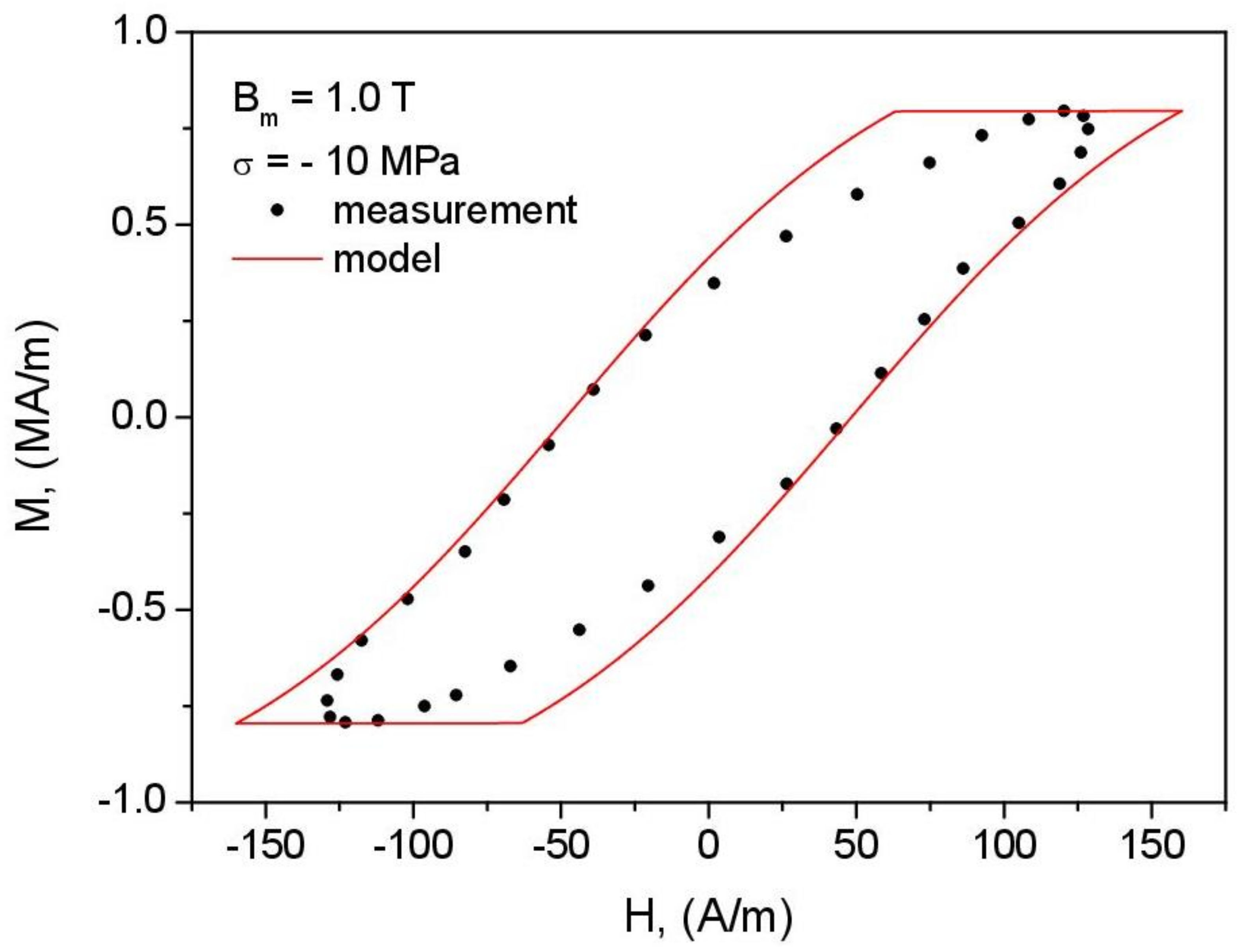
Figure 17, Figure 18, Figure 19 and Figure 20 illustrate the modeling results for several compressive stress values and different induction amplitudes. It can be stated, as a general remark, that despite its simplicity, the stress-dependent Harrison model was able to describe the overall trends observed during the experiment, which confirms its usefulness for engineering purposes.
5. Conclusions
The following conclusions can be drawn:
- The Harrison model has been extended to take into account the effect of compressive stress.
- Despite its highly simplified character, the description has a solid physical background; the anhysteretic curve in this model is truly reversible in the sense of irreversible thermodynamics. Moreover, the description inherently belongs to the class of “inverse” models (Figure 4), which implies that it reflects the real-life excitation conditions in measurement systems complying with international standards.
- It was confirmed that the value of phenomenological parameter introduced by Harrison does depend significantly on the amplitude of minor loop. This value is not affected by the compression pressure. Modeling was carried out for GOES in the range of working induction 1.0–1.5 T. For this material, the values of parameter are higher than (see Figure 11—this can be confronted against the value reported by Harrison in Ref. [10], Figure 18). Parameter , in physical units, and parameter , in reduced units, are inversely proportional; thus, the values of for this induction range exceed 0.785 and quickly rise up to 0.927 for = 1.0 T. This implies practically that the location of bifurcation and switching magnetization values are such that almost whole modeled hysteresis loop branches may be constructed by offsetting the anhysteretic curve by the coercive field value (the sketch in Figure 3 for illustrating the logic of the model refers to non-grain-oriented electrical steel, for which somewhat higher values of coercive field (and consequently lower values) are expected). This implies that the quality of modeling results depends significantly on the correct representation of the anhysteretic curve.
- Two factors affecting the shape of hysteresis loops upon compression were identified: the modified shape of the anhysteretic curve and the increase in coercive field strength. The proposed model extension relied on the introduction of an additional stress-dependent term into the equation that describes the irreversible processes. The anhysteretic curve was identified using a simplified method, and its equation was parametrized. The increase in coercive field strength was accounted for by introducing a power law that considers the applied compressive stress.
- The consequence of the previously formulated conclusion on the effect of correct identification of the anhysteretic curve on the overall performance of the model is the distortion of loop shape for = 1.5 T, = −10 MPa (Figure 19). The highly simplified character of the model (the assumption of only two wells in the Gibbs energy profile as well as the discrepancy between the modeled and reconstructed anhysteretic curves, c.f. Figure 14) contributed to the fact that the model could not describe the complicated loop shape in this case.
- It can be stated that generally, the modeled hysteresis loops are in qualitative agreement with their experimental counterparts. The results might be of interest to the physicists and engineers that cope with the effects of compressive stress on magnetic materials, especially at higher stress values in which buckling may occur. In the published papers focused at the effect of magnetoelastic coupling on the shapes of hysteresis loops, the considered range of compressive stress rarely exceeds 70 MPa because of buckling that occurs in the relatively thin (0.27 mm) GO sheet.
- Future work shall be focused on description fine-tuning as well as on the analysis of the tension case.
Author Contributions
Conceptualization, M.B.d.S.D., F.J.G.L. and K.C.; methodology, M.B.d.S.D. and K.C.; software, K.C.; validation, M.B.d.S.D.; formal analysis, M.B.d.S.D. and F.J.G.L.; investigation, M.B.d.S.D.; resources, M.B.d.S.D.; data curation, M.B.d.S.D., F.J.G.L. and K.C.; writing—original draft preparation, K.C.; writing—review and editing, M.B.d.S.D.; visualization, M.B.d.S.D. and K.C.; supervision, F.J.G.L.; project administration, F.J.G.L.; funding acquisition, K.C. All authors have read and agreed to the published version of the manuscript.
Funding
This research was funded by Fundação de Amparo à Pesquisa do Estado de São Paulo (FAPESP) (grant number # 2017/11645-3) and Conselho Nacional de Desenvolvimento Científico e Tecnológico (CNPq) (grant number # 307631/2018-4).
Institutional Review Board Statement
Not applicable.
Informed Consent Statement
Not applicable.
Data Availability Statement
Data available from the first author upon request.
Acknowledgments
M.B.d.S.D. and F.J.G.L. would like to thank the Fundação de Amparo à Pesquisa do Estado de São Paulo (FAPESP) (grant number # 2017/11645-3) and Conselho Nacional de Desenvolvimento Científico e Tecnológico (CNPq) (grant number # 307631/2018-4) for financial support.
Conflicts of Interest
The authors declare no conflict of interest.
Appendix A. An Analysis of the Harrison Model and MATLAB Code Implementation
Let us examine in detail the ascending branch of the hysteresis loop described with the Harrison model in the quasi-static regime. The reversible term is given with a hyperbolic-tangent-like function; thus, . The irreversible term is given with or .
The coordinates of the bifurcation points are determined by equating , which leads to
The corresponding field strength coordinate is obtained from An inspection of Figure 3 leads to the conclusion that for the ascending loop branch, is negative, whereas takes a positive value. The constant value (coercive field strength) is preserved until a positive value of magnetization is reached (crossing of dash-dotted line with dotted line); this can be determined in Matlab using an anonymous function handle:
Mexit = @(t, hc, m) m-tanh((hc + m)/t)
mexit = fzero(@(m) Mexit(t, -t*atanh(sqrt(1-t)) + sqrt(1-t), m), 1)
% the starting point for iteration is +1, i.e., positive saturation.
Thus, the irreversible curve is composed of three distinct regions:
- (1)
-
where
- (2)
-
where
- (3)
-
where
The descending branch may be obtained from symmetry considerations, using the “flipud” command in MATLAB.
References
- Moses, A.J. The Knowledge of Phenomena Occurring in Magnetic Materials as a Condition to Lower Energy Loss in Magnetic Circuits of Electromagnetic Devices. Available online: https://www.pollub.pl/files/4/attachment/247_Wyklad.pdf (accessed on 30 December 2021).
- Anderson, P.I.; Moses, A.J.; Stanbury, H.J. Assessment of the Stress Sensitivity of Magnetostriction in Grain-Oriented Silicon Steel. IEEE Trans. Magn. 2007, 43, 3467–3476. [Google Scholar] [CrossRef]
- Dias, M.B.S.; Landgraf, F.J.G. Compressive Stress Effects on Magnetic Properties of Uncoated Grain Oriented Electrical Steel. J. Magn. Magn. Mater. 2020, 504, 166566. [Google Scholar] [CrossRef]
- Perevertov, O.; Schäfer, R. Magnetic Properties and Magnetic Domain Structure of Grain-Oriented Fe-3%Si Steel under Compression. Mater. Res. Express 2016, 3, 096103. [Google Scholar] [CrossRef]
- Anderson, P. Measurement of the Stress Sensitivity of Magnetostriction in Electrical Steels under Distorted Waveform Conditions. J. Magn. Magn. Mater. 2008, 320, e583–e588. [Google Scholar] [CrossRef]
- Li, J.; Xu, M. Modified Jiles-Atherton-Sablik Model for Asymmetry in Magnetomechanical Effect under Tensile and Compressive Stress. J. Appl. Phys. 2011, 110, 063918. [Google Scholar] [CrossRef]
- Shi, P.; Jin, K.; Zheng, X. A General Nonlinear Magnetomechanical Model for Ferromagnetic Materials under a Constant Weak Magnetic Field. J. Appl. Phys. 2016, 119, 145103. [Google Scholar] [CrossRef]
- Aydin, U.; Rasilo, P.; Martin, F.; Singh, D.; Daniel, L.; Belahcen, A.; Rekik, M.; Hubert, O.; Kouhia, R.; Arkkio, A. Magneto-Mechanical Modeling of Electrical Steel Sheets. J. Magn. Magn. Mater. 2017, 439, 82–90. [Google Scholar] [CrossRef]
- Matsuo, T.; Takahashi, Y.; Fujiwara, K. Pinning Field Representation Using Play Hysterons for Stress-Dependent Domain-Structure Model. J. Magn. Magn. Mater. 2020, 499, 166303. [Google Scholar] [CrossRef]
- Harrison, R.G. A Physical Model of Spin Ferromagnetism. IEEE Trans. Magn. 2003, 39, 950–960. [Google Scholar] [CrossRef]
- Preisach, F. On the magnetic aftereffect. IEEE Trans. Magn. 2017, 53, 0700111, (translation of the German text published in Z. Phys. 1935, 94, 277–302). [Google Scholar] [CrossRef]
- Mayergoyz, I.D. Mathematical Models of Hysteresis and Their Applications, 2nd ed.; Academic Press, Elsevier: San Diego, CA, USA, 2003. [Google Scholar] [CrossRef] [Green Version]
- Sumarac, D.; Knezevic, P.; Dolicanin, C.; Cao, M. Preisach Elasto-Plastic Model for Mild Steel Hysteretic Behavior-Experimental and Theoretical Considerations. Sensors 2021, 21, 3546. [Google Scholar] [CrossRef]
- Im, S.-H.; Lee, H.-Y.; Park, G.-S. Novel Deperming Protocols to Reduce Demagnetizing Time and Improve the Performance for the Magnetic Silence of Warships. Energies 2021, 14, 6295. [Google Scholar] [CrossRef]
- Jiles, D.; Atherton, D. Ferromagnetic Hysteresis. IEEE Trans. Magn. 1983, 19, 2183–2185. [Google Scholar] [CrossRef]
- Jiles, D.C.; Atherton, D.L. Theory of Ferromagnetic Hysteresis. J. Magn. Magn. Mater. 1986, 61, 48–60. [Google Scholar] [CrossRef]
- Zirka, S.E.; Moroz, Y.I.; Harrison, R.G.; Chwastek, K. On Physical Aspects of the Jiles-Atherton Hysteresis Models. J. Appl. Phys. 2012, 112, 043916. [Google Scholar] [CrossRef]
- Jastrzębski, R.; Chwastek, K. Comparison of Macroscopic Descriptions of Magnetization Curves. In Proceedings of the ITM Web of Conferences, Lublin, Poland, 23–25 November 2017; Volume 15, p. 03003. [Google Scholar]
- Cao, W. Constructing Landau-Ginzburg-Devonshire type models for ferroelectric systems based on symmetry. Ferroelectrics 2008, 375, 28–39. [Google Scholar] [CrossRef]
- Catalan, G.; Jiménez, D.; Gruverman, A. Ferroelectrics: Negative capacitance detected. Nat. Mater. 2015, 14, 137–139. [Google Scholar] [CrossRef]
- Íñiguez, J.; Zubko, P.; Luk’yanchuk, I.; Cano, A. Ferroelectric negative capacitance. Nat. Rev. Mater. 2019, 4, 243–256. [Google Scholar] [CrossRef] [Green Version]
- Hoffmann, M.; Fengler, F.P.G.; Herzig, M.; Mittmann, T.; Max, B.; Schroeder, U.; Negrea, R.; Lucian, P.; Slesazeck, S.; Mikolajick, T. Unveiling the double-well energy landscape in a ferroelectric layer. Nature 2019, 565, 464–467. [Google Scholar] [CrossRef]
- Morozzi, A.; Hoffmann, M.; Mulargia, R.; Slesazeck, S.; Robutti, E. Negative capacitance devices: Sensitivity analyses of the developed TCAD ferroelectric model for HZO. J. Instrument. 2022, 17, C01048. [Google Scholar] [CrossRef]
- Bertotti, G. Hysteresis in Magnetism; Academic Press: San Diego, CA, USA, 1998. [Google Scholar]
- Gębara, P.; Gozdur, R.; Chwastek, K. The Harrison Model as a Tool to Study Phase Transitions in Magnetocaloric Materials. Acta Phys. Pol. A 2018, 134, 1217–1220. [Google Scholar] [CrossRef]
- Fabrizio, M.; Giorgi, C.; Morro, A. A thermodynamic approach to ferromagnetism and phase transitions. Int. J. Eng. Sci. 2009, 47, 821–839. [Google Scholar] [CrossRef]
- Kochmański, M.; Paszkiewicz, T.; Wolski, S. Curie-Weiss magnet—A simple model of phase transition. Eur. J. Phys. 2013, 34, 1555. [Google Scholar] [CrossRef] [Green Version]
- Berti, A.; Giorgi, C.; Vuk, E. Hysteresis and temperature-induced transitions in ferromagnetic materials. Appl. Math. Model. 2015, 39, 820–837. [Google Scholar] [CrossRef]
- Koksharov, Y.A. Analytic solutions of the Weiss mean field equation. J. Magn. Magn. Mater. 2020, 516, 167179. [Google Scholar] [CrossRef]
- Helmiss, G.; Storm, L. Movement of an individual Bloch wall in single-crystal picture frame of silicon iron at very low velocities. IEEE Trans. Magn. 1974, 10, 36–38. [Google Scholar] [CrossRef]
- Grosse-Nobis, W. Frequency spectrum of the Barkhausen noise of a moving 180° domain wall. J. Magn. Magn. Mater. 1977, 4, 247–253. [Google Scholar] [CrossRef]
- Chwastek, K.; Gozdur, R. Towards a Unified Approach to Hysteresis and Micromagnetics Modeling: A Dynamic Extension to the Harrison Model. Phys. B Condens. Matter 2019, 572, 242–246. [Google Scholar] [CrossRef]
- Haller, T.R.; Kramer, J.J. Observation of Dynamic Domain Size Variation in a Silicon-Iron Alloy. J. Appl. Phys. 1970, 41, 1034–1035. [Google Scholar] [CrossRef]
- Cohen, A. A Padé Approximant to the Inverse Langevin Function. Rheol. Acta 1991, 30, 270–273. [Google Scholar] [CrossRef]
- Tumanski, S. Handbook of Magnetic Measurements; CRC Press: Boca Raton, FL, USA, 2011. [Google Scholar]
- Daniel, L.; Domenjoud, M. Anhysteretic magneto-elastic behaviour of Terfenol-D: Experiments, multiscale modeling and analytical formulas. Materials 2021, 14, 5165. [Google Scholar] [CrossRef] [PubMed]
- Krah, J.H.; Bergqvist, A.J. Numerical Optimization of a Hysteresis Model. Phys. B Condens. Matter 2004, 343, 35–38. [Google Scholar] [CrossRef]
- Schneider, C.S.; Cannell, P.Y.; Watts, K.T. Magnetoelasticity for Large Stresses. IEEE Trans. Magn. 1992, 28, 2626–2631. [Google Scholar] [CrossRef]
- Schimid, E.; Boas, W. Plasticity of Crystals; F. A. Hughes & Co., Ltd.: London, UK, 1950. [Google Scholar]
- Kobayashi, S.; Takahashi, S.; Kamada, Y.; Kikuchi, H. A Low-Field Scaling Rule of Minor Hysteresis Loops in Plastically Deformed Steels. IEEE Trans. Magn. 2010, 46, 191–194. [Google Scholar] [CrossRef]
- Chwastek, K. Modelling Offset Minor Hysteresis Loops with the Modified Jiles-Atherton Description. J. Phys. D Appl. Phys. 2009, 42, 165002. [Google Scholar] [CrossRef]
- Franco, V.; Blázquez, J.S.; Ingale, B.; Conde, A. The Magnetocaloric Effect and Magnetic Refrigeration Near Room Temperature: Materials and Models. Annu. Rev. Mater. Res. 2012, 42, 305–342. [Google Scholar] [CrossRef] [Green Version]
- Gębara, P.; Hasiak, M. Determination of Phase Transition and Critical Behavior of the As-Cast GdGeSi-(X) Type Alloys (Where X = Ni, Nd and Pr). Materials 2021, 14, 185. [Google Scholar] [CrossRef]
- Allia, P.; Coisson, M.; Tiberto, P.; Vinai, F.; Knobel, M.; Novak, M.; Nunes, W. Granular Cu-Co Alloys as Interacting Superparamagnets. Phys. Rev. B 2001, 64, 144420. [Google Scholar] [CrossRef] [Green Version]
- Gozdur, R.; Najgebauer, M. Scaling analysis of phase transitions in magnetocaloric alloys. J. Magn. Magn. Mater. 2020, 499, 166239. [Google Scholar] [CrossRef]
- Harrison, R.G. Variable-Domain-Size Theory of Spin Ferromagnetism. IEEE Trans. Magn. 2004, 40, 1506–1515. [Google Scholar] [CrossRef]
- Chwastek, K.; Szczygłowski, J. An Alternative Method to Estimate the Parameters of Jiles–Atherton Model. J. Magn. Magn. Mater. 2007, 314, 47–51. [Google Scholar] [CrossRef]
- Bertotti, G.; Basso, V. Considerations on the Physical Interpretation of the Preisach Model of Ferromagnetic Hysteresis. J. Appl. Phys. 1993, 73, 5827–5829. [Google Scholar] [CrossRef]
- Raghunathan, A.; Melikhov, Y.; Snyder, J.E.; Jiles, D.C. Modeling of Two-Phase Magnetic Materials Based on Jiles–Atherton Theory of Hysteresis. J. Magn. Magn. Mater. 2012, 324, 20–22. [Google Scholar] [CrossRef]
- Raghunathan, A.; Klimczyk, P.; Melikhov, Y. Application of Jiles-Atherton Model to Stress Induced Magnetic Two-Phase Hysteresis. IEEE Trans. Magn. 2013, 49, 3187–3190. [Google Scholar] [CrossRef]
- Baghel, A.P.S.; Sai Ram, B.; Chwastek, K.; Daniel, L.; Kulkarni, S.V. Hysteresis Modelling of GO Laminations for Arbitrary In-Plane Directions Taking into Account the Dynamics of Orthogonal Domain Walls. J. Magn. Magn. Mater. 2016, 418, 14–20. [Google Scholar] [CrossRef]
- Baghel, A.P.S.; Kulkarni, S.V. Hysteresis Modeling of the Grain-Oriented Laminations with Inclusion of Crystalline and Textured Structure in a Modified Jiles-Atherton Model. J. Appl. Phys. 2013, 113, 043908. [Google Scholar] [CrossRef]
- Perevertov, O.; Schaefer, R.; Stupakov, O. 3-D Branching of Magnetic Domains on Compressed Si-Fe Steel with Goss Texture. IEEE Trans. Magn. 2014, 50, 2007804. [Google Scholar] [CrossRef]
- Baghel, A.P.S.; Chwastek, K.; Kulkarni, S.V. Modelling of Minor Hysteresis Loops in Rolling and Transverse Directions of Grain-oriented Laminations. IET Electr. Power Appl. 2015, 9, 344–348. [Google Scholar] [CrossRef]
- Klimczyk, P. Novel Techniques for Characterisation and Control of Magnetostriction in G.O.S.S. Ph.D. Thesis, Cardiff University, Cardiff, UK, 2012. [Google Scholar]
- Sablik, M.J.; Kwun, H.; Burkharddt, G.L.; Jiles, D.C. Model for the Effect of Tensile and Compressive Stress on Ferromagnetic Hysteresis. J. Appl. Phys. 1987, 61, 3799–3801. [Google Scholar] [CrossRef]
- Sablik, M.J.; Jiles, D.C. Coupled Magnetoelastic Theory of Magnetic and Magnetostrictive Hysteresis. IEEE Trans. Magn. 1993, 29, 2113–2123. [Google Scholar] [CrossRef] [Green Version]
- M’zali, N.; Martin, F.; Aydin, U.; Belahcen, A.; Benabou, A.; Henneron, T. Determination of Stress Dependent Magnetostriction from a Macroscopic Magneto-Mechanical Model and Experimental Magnetization Curves. J. Magn. Magn. Mater. 2020, 500, 166299. [Google Scholar] [CrossRef]
- Vicena, F. On the Connection between the Coercive Force of a Ferromagnetic and Internal Stress. Czechosl. J. Phys. 1954, 4, 419–436. (In Russian) [Google Scholar] [CrossRef]
- Málek, Z. The Dependence of Coercive Force on Plastic Deformation. Czechosl. J. Phys. 1957, 7, 152–167. (In German) [Google Scholar] [CrossRef]
- Qureshi, A.H.; Chaudhary, L.N. Influence of Plastic Deformation on Coercive Field and Initial Susceptibility of Fe-3.25% Si Alloys. J. Appl. Phys. 1970, 41, 1042–1043. [Google Scholar] [CrossRef]
- Timofeev, I.A.; Kustov, E.F. To the Theory of Dynamic Magnetization and Magnetic Reversal of a Ferromagnet. Russ. Phys. J. 2006, 49, 260–267. [Google Scholar] [CrossRef]
- Moses, A.J. Energy Efficient Electrical Steels: Magnetic Performance Prediction and Optimization. Scr. Mater. 2012, 67, 560–565. [Google Scholar] [CrossRef]
- Dias, M.B.S.; Bentancour, D.P.M.; Araújo, F.G.P.; Santos, A.D.; Landgraf, F.J.G. Power Loss Reduction of Uncoated Grain Oriented Electrical Steel Using Annealing under Stress Treatment. J. Magn. Magn. Mater. 2020, 504, 166632. [Google Scholar] [CrossRef]
- Sablik, M.J. A Model for Asymmetry in Magnetic Property Behavior under Tensile and Compressive Stress in Steel. IEEE Trans. Magn. 1997, 33, 3958–3960. [Google Scholar] [CrossRef]
Figure 1.
The impact of magnetic field strength on the variation of Gibbs free energy profile for an arbitrarily chosen temperature (t = 0.8) in the Landau theory. An illustrative depiction.
Figure 1.
The impact of magnetic field strength on the variation of Gibbs free energy profile for an arbitrarily chosen temperature (t = 0.8) in the Landau theory. An illustrative depiction.

Figure 2.
The correspondence between the double-well energy profile and the irreversible hysteresis loop due to internal positive feedback. Source: own work, based on the concept from [22].
Figure 2.
The correspondence between the double-well energy profile and the irreversible hysteresis loop due to internal positive feedback. Source: own work, based on the concept from [22].
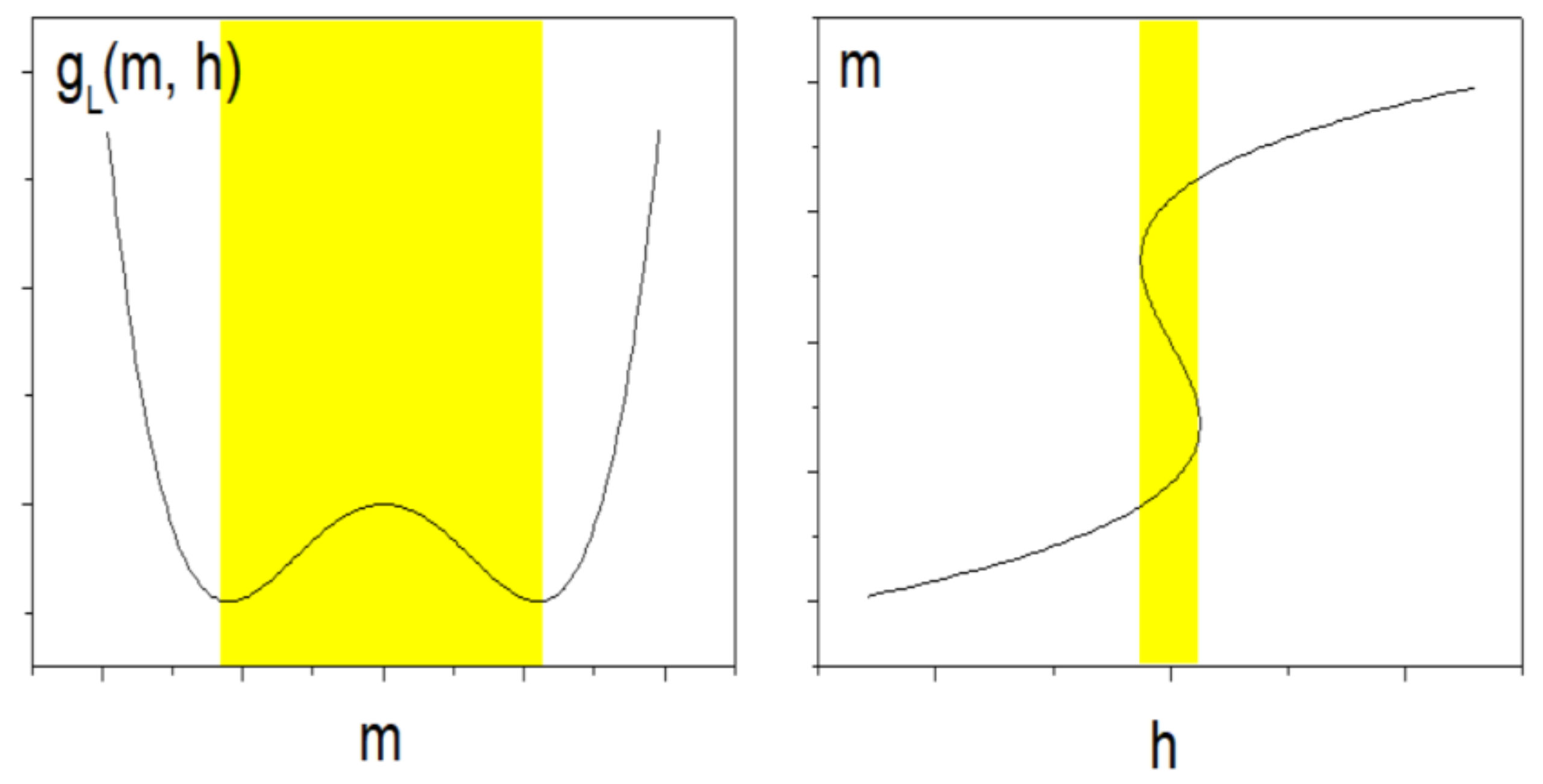
Figure 3.
Summation of field strength contributions in the Harrison model. Source: own work, based on the concept from [10].
Figure 3.
Summation of field strength contributions in the Harrison model. Source: own work, based on the concept from [10].
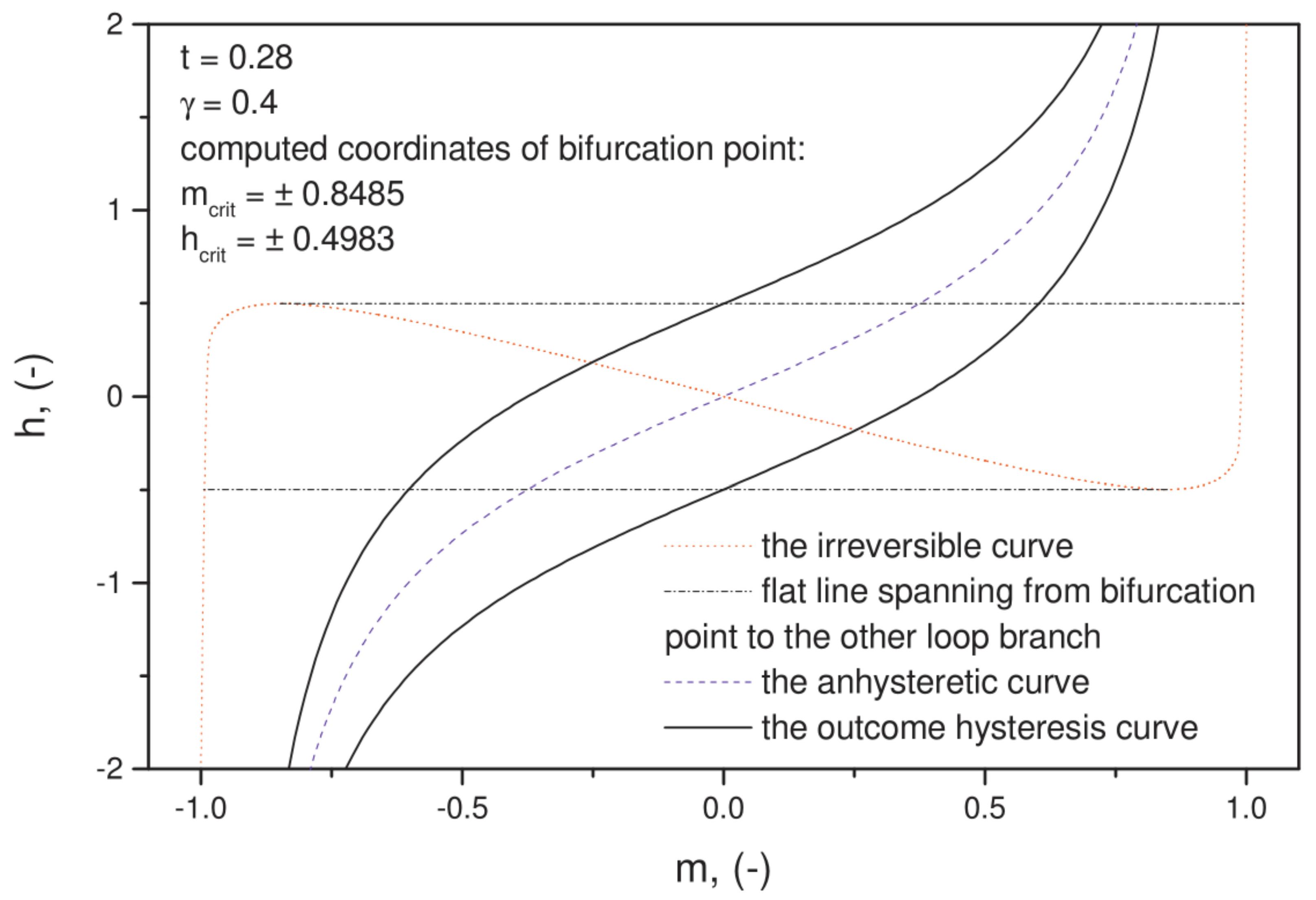
Figure 4.
Computation chain for (a) the simple and (b) for the inverse hysteresis model.
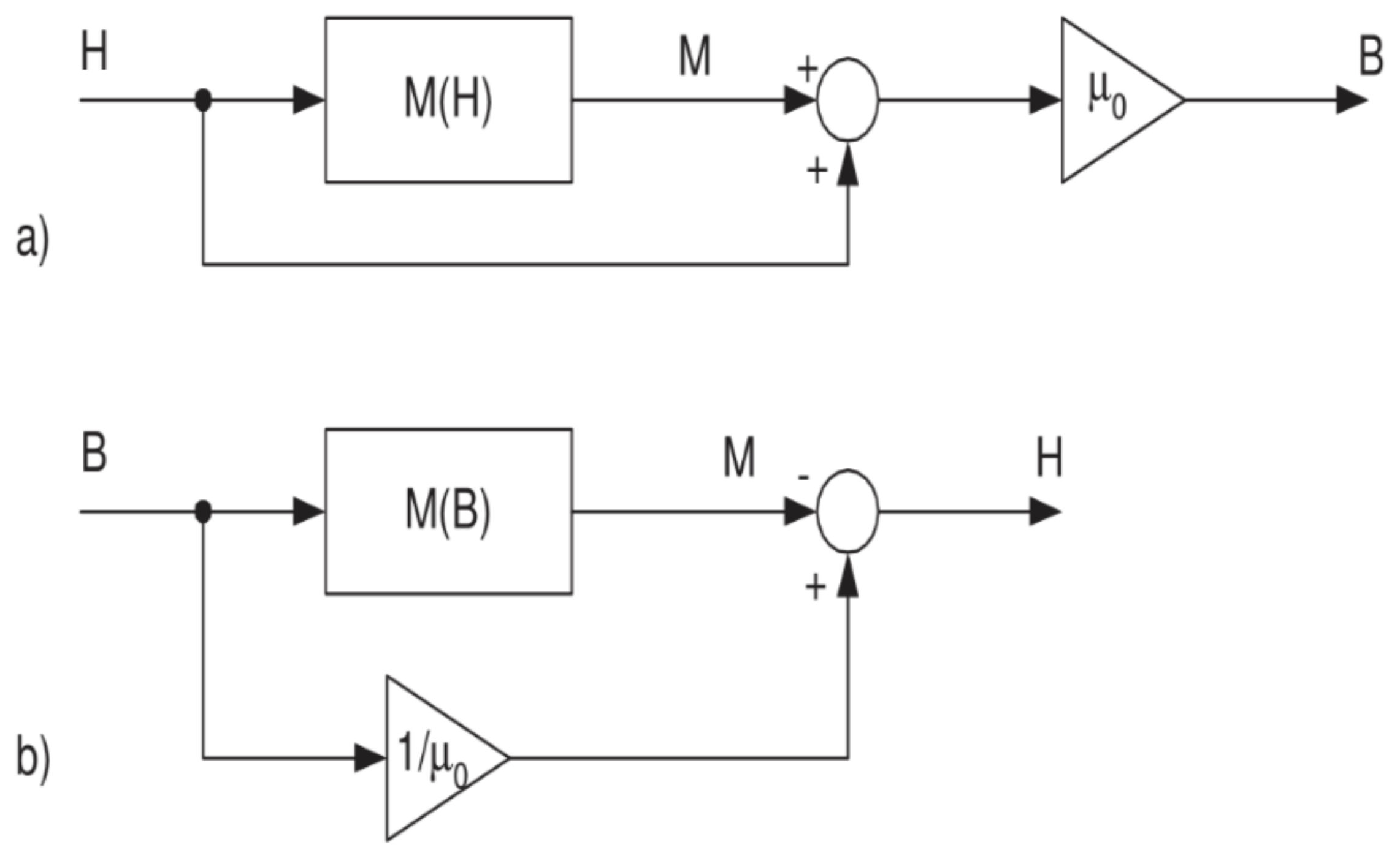
Figure 5.
An approximate method to determine the anhysteretic curve. An illustrative depiction.

Figure 6.
A photograph of the experimental setup that was used to measure hysteresis loops with SST and NI board (USB-6259) that acquired H and B experimental data.
Figure 6.
A photograph of the experimental setup that was used to measure hysteresis loops with SST and NI board (USB-6259) that acquired H and B experimental data.
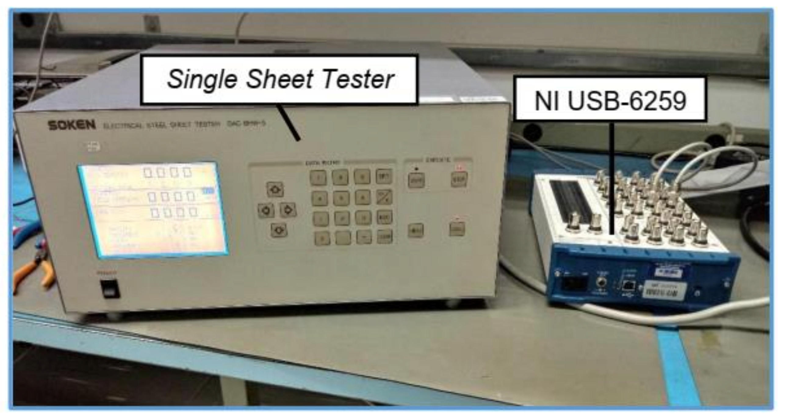
Figure 7.
Photograph of the frame used to apply compressive stress in the GOES sample and (a) frame attached on SST during magnetic measurement (b).
Figure 7.
Photograph of the frame used to apply compressive stress in the GOES sample and (a) frame attached on SST during magnetic measurement (b).

Figure 8.
A photograph of Wheatstone bridge components used to measure the strain of the samples under stress.
Figure 8.
A photograph of Wheatstone bridge components used to measure the strain of the samples under stress.
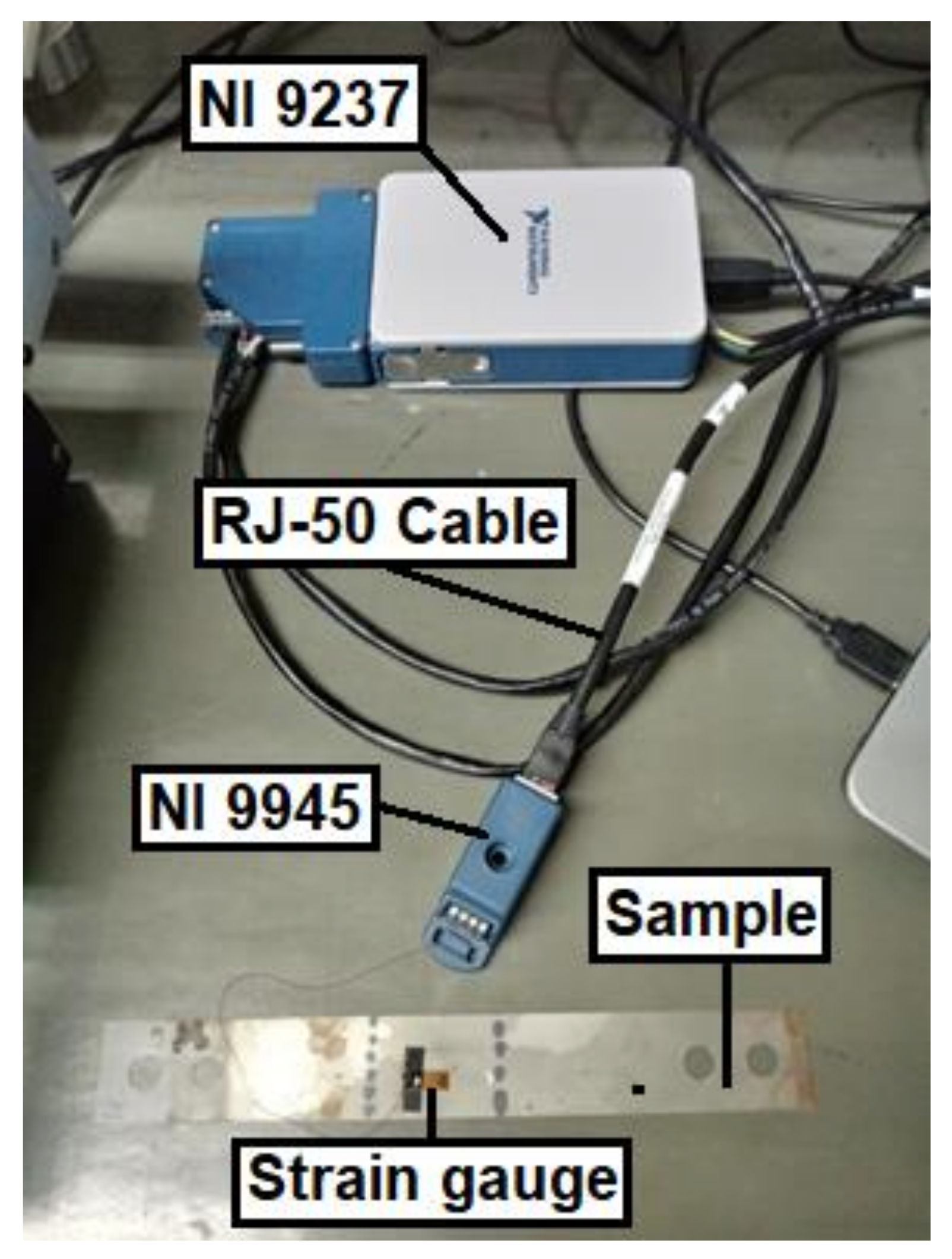
Figure 9.
Fitting of recovered anhysteretic curves with the hyperbolic tangent function, free parameters.
Figure 9.
Fitting of recovered anhysteretic curves with the hyperbolic tangent function, free parameters.
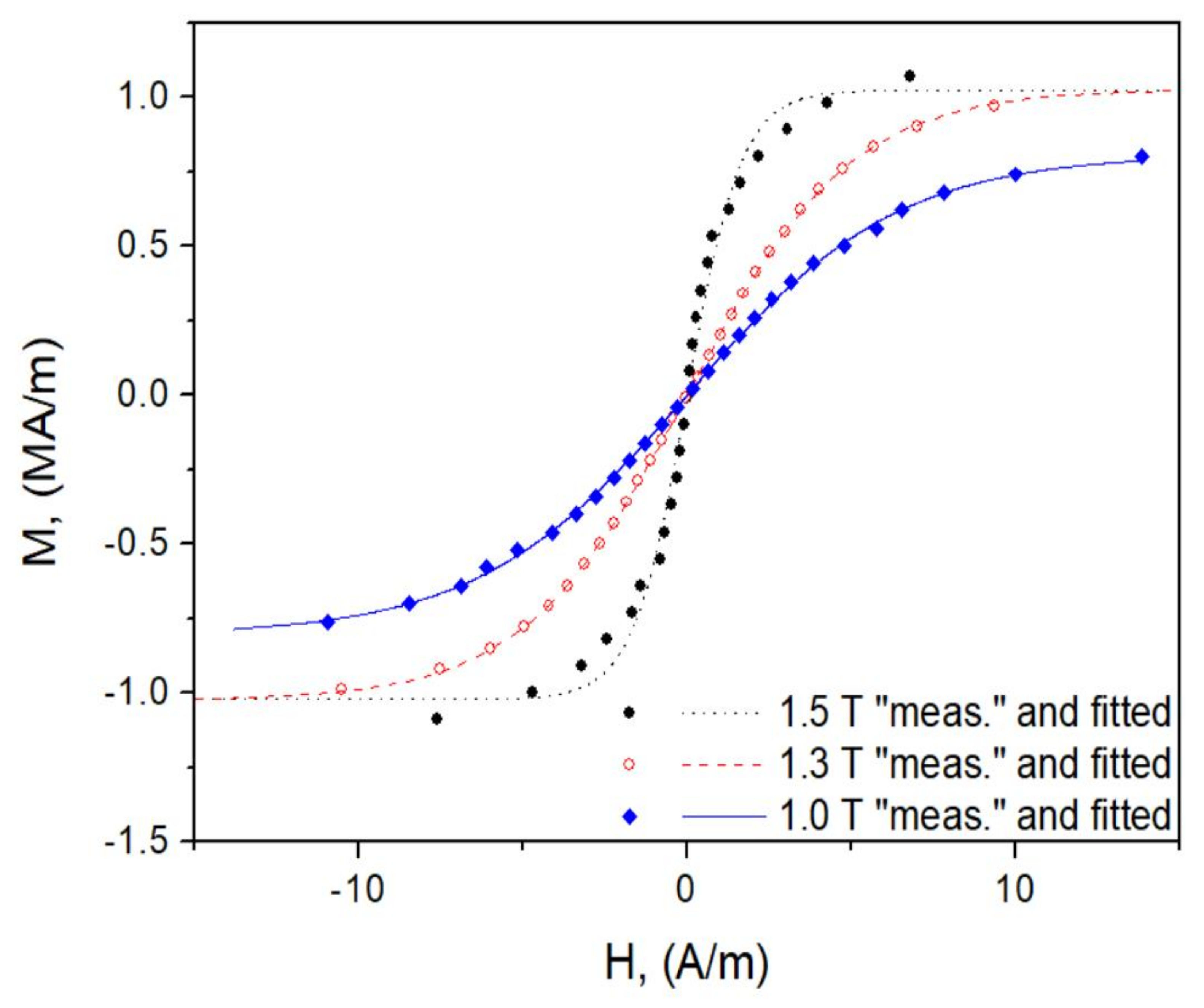
Figure 10.
Fitting of anhysteretic curves according to Formula (1).

Figure 11.
The measured values of coercive field strength and computed values of parameter .

Figure 12.
The measured and the modeled minor hysteresis loop for T.
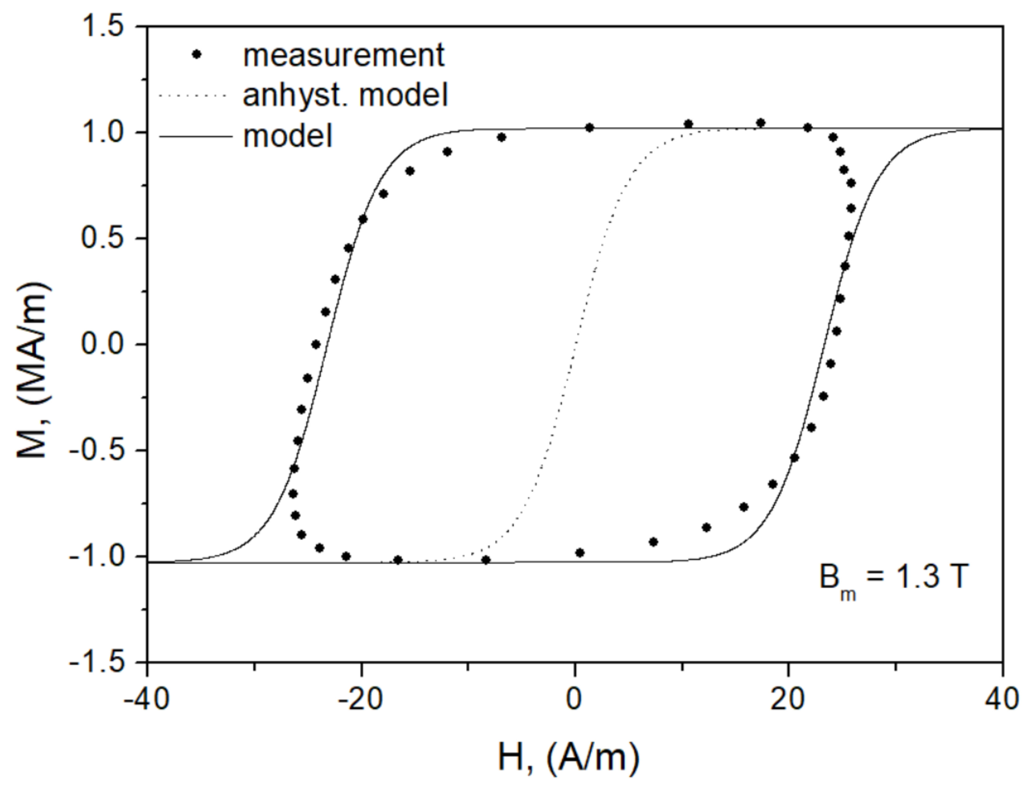
Figure 13.
Experimental hysteresis curves: dotted line—for σ = 0 MPa, dashed line—for compressive stress σ = −10 MPa.
Figure 13.
Experimental hysteresis curves: dotted line—for σ = 0 MPa, dashed line—for compressive stress σ = −10 MPa.
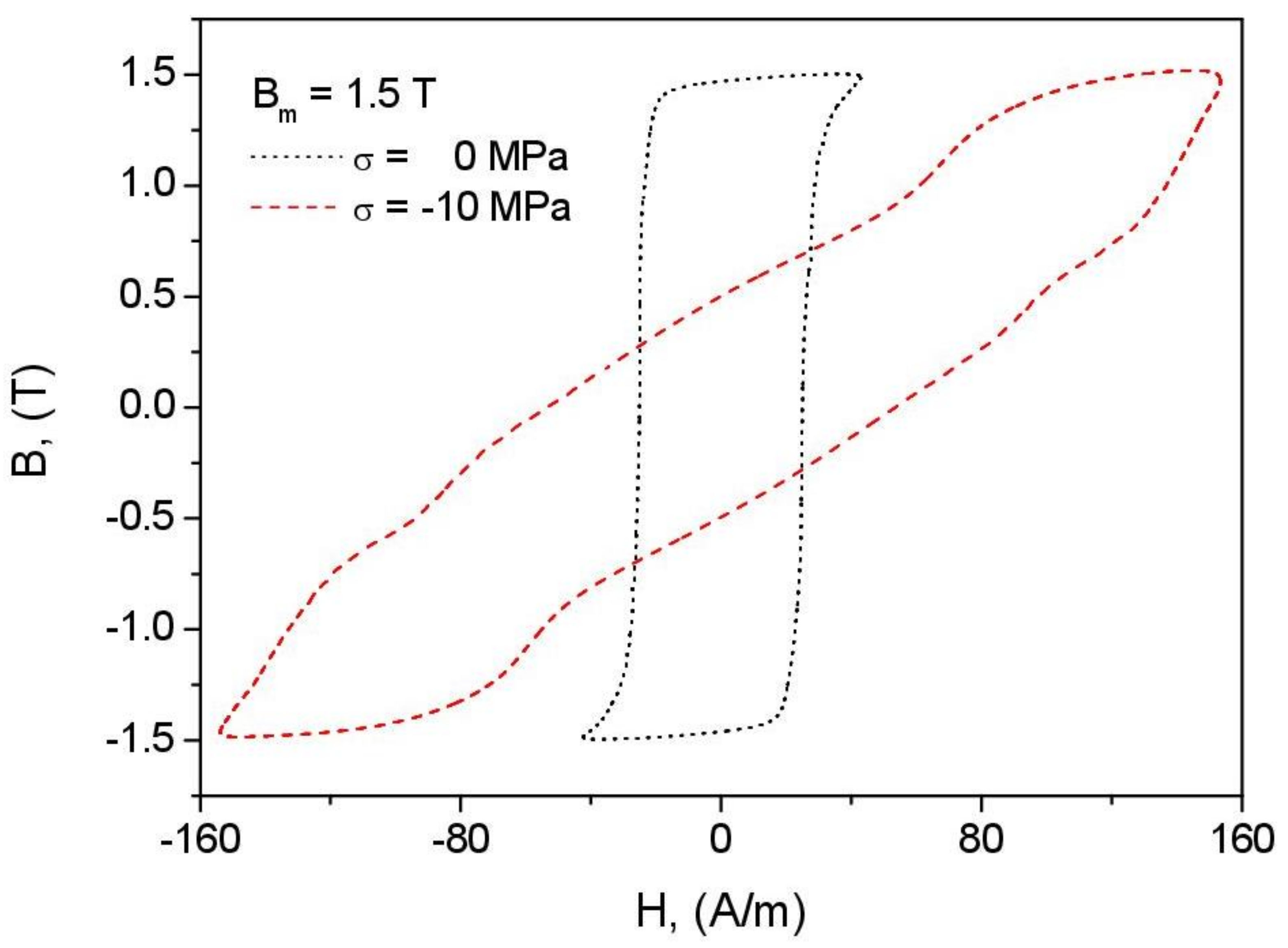
Figure 14.
Anhysteretic curves recovered as the middle curves of measured hysteresis loops and modeled using Equation (2) for chosen values of compressive stress.
Figure 14.
Anhysteretic curves recovered as the middle curves of measured hysteresis loops and modeled using Equation (2) for chosen values of compressive stress.
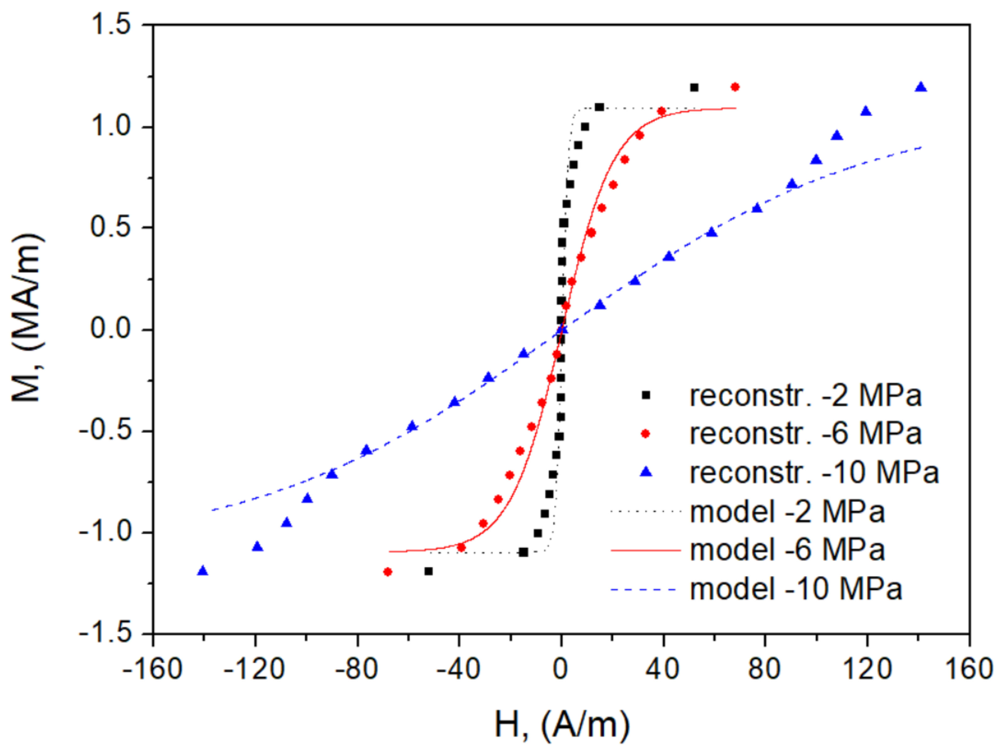
Figure 15.
Photograph of GOES structure, showing the grain boundaries (dotted lines), pick-up coil area (red square), and the spot where strain gauge was glued.
Figure 15.
Photograph of GOES structure, showing the grain boundaries (dotted lines), pick-up coil area (red square), and the spot where strain gauge was glued.

Figure 16.
Measured and modeled dependence of excess coercive field strength on compression pressure at Bm = 1.5 T. Moreover, the simulated trend for k = 0.1 is also shown (concerns tension).
Figure 16.
Measured and modeled dependence of excess coercive field strength on compression pressure at Bm = 1.5 T. Moreover, the simulated trend for k = 0.1 is also shown (concerns tension).
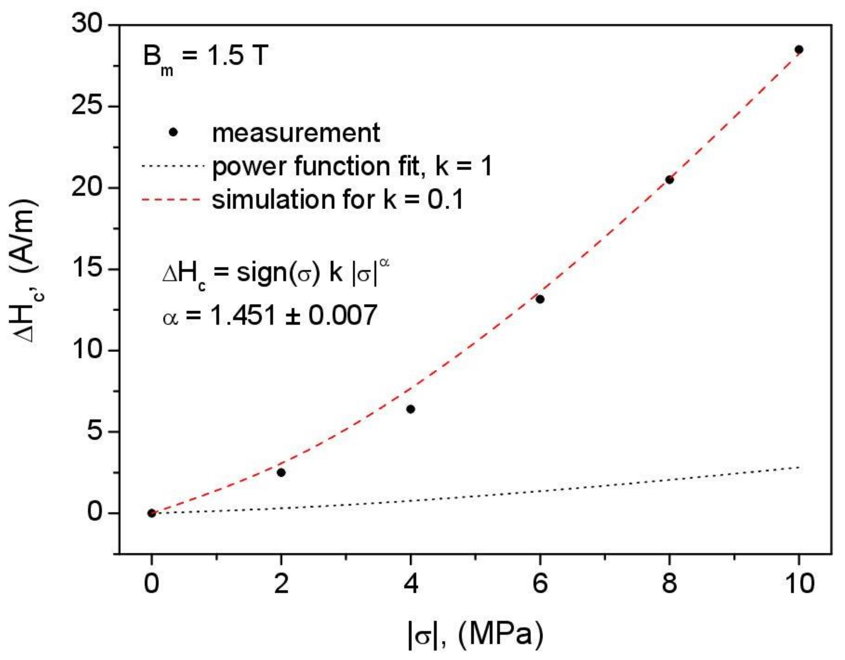
Figure 17.
Measured and modeled hysteresis loops for σ = −2 MPa, Bm = 1.5 T.
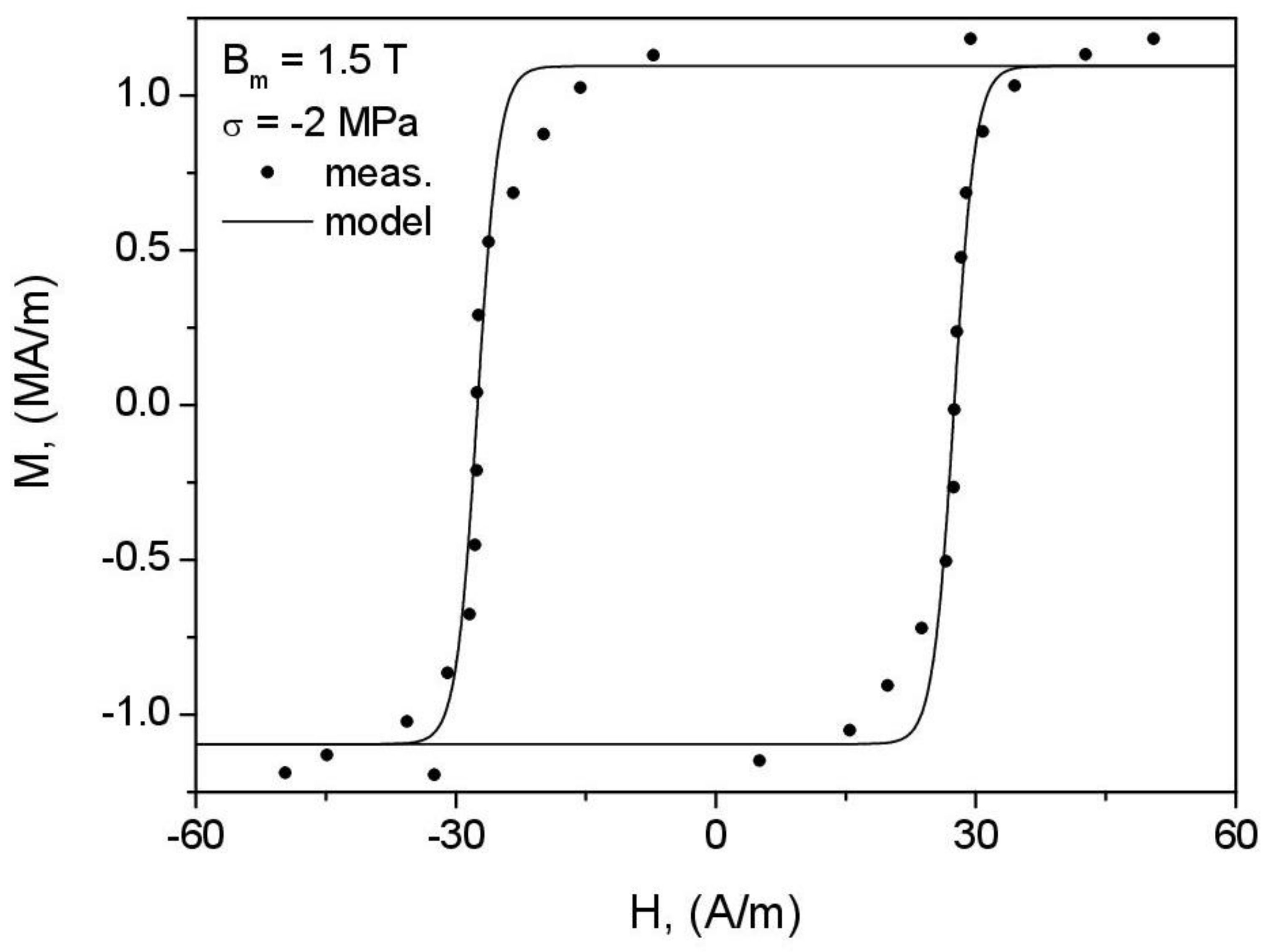
Figure 18.
Measured and modeled hysteresis loops for σ = −6 MPa, Bm = 1.5 T.
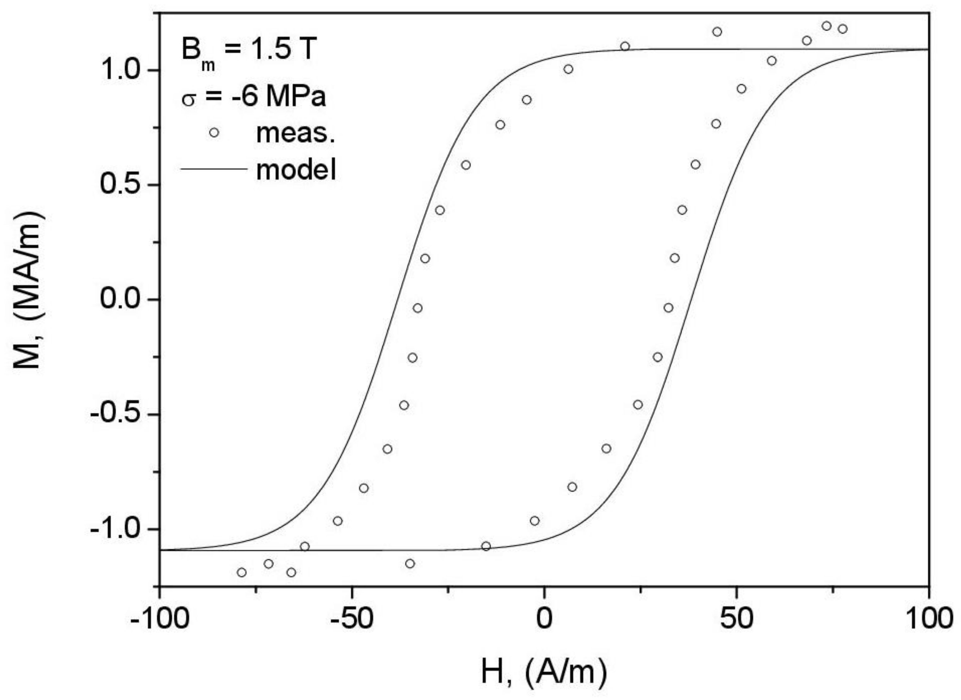
Figure 19.
Measured and modeled hysteresis loops for σ = −10 MPa, Bm = 1.5 T.

Figure 20.
Measured and modeled hysteresis loops for σ = −10 MPa, Bm = 1.0 T.
Publisher’s Note: MDPI stays neutral with regard to jurisdictional claims in published maps and institutional affiliations. |
© 2022 by the authors. Licensee MDPI, Basel, Switzerland. This article is an open access article distributed under the terms and conditions of the Creative Commons Attribution (CC BY) license (https://creativecommons.org/licenses/by/4.0/).
Share and Cite
MDPI and ACS Style
de Souza Dias, M.B.; Landgraf, F.J.G.; Chwastek, K. Modeling the Effect of Compressive Stress on Hysteresis Loop of Grain-Oriented Electrical Steel. Energies 2022, 15, 1128. https://doi.org/10.3390/en15031128
AMA Style
de Souza Dias MB, Landgraf FJG, Chwastek K. Modeling the Effect of Compressive Stress on Hysteresis Loop of Grain-Oriented Electrical Steel. Energies. 2022; 15(3):1128. https://doi.org/10.3390/en15031128
Chicago/Turabian Stylede Souza Dias, Mateus Botani, Fernando José Gomes Landgraf, and Krzysztof Chwastek. 2022. "Modeling the Effect of Compressive Stress on Hysteresis Loop of Grain-Oriented Electrical Steel" Energies 15, no. 3: 1128. https://doi.org/10.3390/en15031128
Note that from the first issue of 2016, this journal uses article numbers instead of page numbers. See further details here.