
Polarization Voltage Characterization of Lithium-Ion Batteries Based on a Lumped Diffusion Model and Joint Parameter Estimation Algorithm


Division of Advanced Manufacturing, Shenzhen International Graduate School, Tsinghua University, Shenzhen 518055, China
*
Author to whom correspondence should be addressed.
Energies 2022, 15(3), 1150; https://doi.org/10.3390/en15031150
Submission received: 12 January 2022
/
Revised: 28 January 2022
/
Accepted: 31 January 2022
/
Published: 4 February 2022
(This article belongs to the Topic Energy Storage and Conversion Systems)
Abstract
:Polarization is a universal phenomenon that occurs inside lithium-ion batteries especially during operation, and whether it can be accurately characterized affects the accuracy of the battery management system. Model-based approaches are commonly adopted in studies of the characterization of polarization. Towards the application of the battery management system, a lumped diffusion model with three parameters was adopted. In addition, a joint algorithm composed of the Particle Swarm Optimization algorithm and the Levenberg-Marquardt method is proposed to identify model parameters. Verification experiments showed that this proposed algorithm can significantly improve the accuracy of model output voltages compared to the Particle Swarm Optimization algorithm alone and the Levenberg-Marquardt method alone. Furthermore, to verify the real-time performance of the proposed method, a hardware implementation platform was built, and this system’s performance was tested under actual operating conditions. Results show that the hardware platform is capable of realizing the basic function of quantitative polarization voltage characterization, and the updating frequency of relevant parameters can reach 1 Hz, showing good real-time performance.
1. Introduction
Due to the high operating voltage and high energy density of lithium-ion batteries, both grid and off-grid applications using lithium-ion batteries have gained a lot of attention [1], especially in the field of electric vehicles [2]. In addition to the advancement of battery manufacturing technology, a sufficiently accurate and agile battery management system (BMS) is important for the further application of lithium-ion batteries [3].
During battery charge/discharge cycles, the external characteristics of batteries behave as a time-varying nonlinear system due to the nonlinear relationship between electric potential versus State of Charge (SOC), as well as the voltage drop due to various polarization phenomena (e.g., ohmic polarization, activation polarization, concentration polarization) [4]. It is important to clarify that polarization is a universal phenomenon that occurs inside the lithium-ion battery during operation, with different types of polarization occurring at different locations inside the battery. Furthermore, the relative proportion of each type of polarization varies with the change of external excitation [5]. Polarization hinders lithium intercalation and deintercalation kinetics, leading to a decline in energy efficiency and performance of the battery [6]. Therefore, polarization is of concern during the entire phase from battery material development to the end-of-life phase of batteries. In addition, higher charge/discharge rates, extremely low ambient temperatures, and increased cycles, which are common scenarios encountered during the use of power batteries, can all lead to increased battery polarization [7].
Polarization is concerned in different stages of battery development and application.
- (i.)
- In the cell design phase, improvements are made for the internal composition of the cell. Zheng et al. pointed out that polarization leads to uneven distribution of electrode active material, which causes performance decline for lithium-ion batteries [6]. The separator is a key component inside a lithium-ion battery cell. Feng et al. redeveloped the separator material to mitigate the polarization phenomenon during battery operation, which enhanced the power performance and cycling stability of the battery [8]. Kim et al. improved the anode materials for lithium-ion batteries to mitigate the polarization phenomenon of lithium-ion batteries during operation [9]. In [10], Shi et al. prepared an electrical conductive graphene nanosheet with hybrid lithium titanate nanoparticles dispersed on it as an anode, which shortened the ion transport path, greatly improving the ion and electron transport efficiency at the particle/electrolyte coupling interface, and remarkably reducing the charge transfer impedance, and improving the battery cycling performance under large rate conditions. The DRT (Distribution of Relaxation Times) method has been used to analyze the impedance spectrum of lithium-ion batteries in the frequency domain to precisely characterize various types of polarization, and used to develop new cathode materials [11]. Song et al. developed a ferroelectric polyvinylidene difluoride (PVDF) polymer as a binder material and demonstrated by the galvanostatic intermittent titration technique (GITT) measurement and in situ galvanostatic electrochemical impedance spectroscopy (GS-EIS) analysis that this new material can significantly reduce the lithium-ion diffusion impendence as a binder inside cells, compared to the paraelectric PVDF binder material, thereby improving the battery performance under large rate conditions. This provided new inspiration for the design of high-performance lithium-ion batteries [12].
- (ii.)
- Polarization has been considered an influential factor in numerous studies related to the thermal management system of lithium-ion batteries. In [13], the respective proportion of ohmic internal resistance and polarization internal resistance under different discharge rate conditions were explored to summarize the contribution of polarization in the accumulation of internal battery temperature at the early stage of thermal runaway, which provides a theoretical basis for safer battery design. As discussed in [14,15], the heat of polarization is the main component of the internal heat production of the cell and consists of four parts: ohmic heat, polarization heat, reaction heat, and side-reaction heat. Taheri P, Mansouri A et al. developed a two-dimensional analytical model of the lithium-ion battery, and a concentration-independent polarization voltage was derived to explore the application for battery thermal management through the thermal coupling model [16]. Goonetilleke D. et al. found that increasing the ambient temperature increased the reaction rate inside the battery and reduced polarization inside battery cells [17]. In [18], the optimal alternating current (AC) frequency was determined based on the Thevenin-thermal coupling model in the frequency domain, and an internal heating strategy based on a constant polarization voltage at low ambient temperatures was developed, which achieved a good balance between cell aging and heating efficiency.
- (iii.)
- State of Charge and State of Health (SOH) are two very important state parameters in BMS, and the influence of polarization on estimation accuracy cannot be ignored. Li et al. pointed out that polarization resistance contributes significantly to the battery capacity decay, so the accurate characterization of polarization is important for developing the estimation method of SOH [19]. Marino C. et al. quantified the electrode polarization resistance and established a functional relationship with the external current excitation at different cycle rates to estimate the aging state of the battery to determine battery failure [20]. SOH decays with increasing cycle number, and Xia and Chen et al. defined the concept of Degree of Polarization (DOP) to correct SOH estimation results to improve the accuracy of SOC estimation [21].
- (iv.)
- In battery charging technology, polarization is also considered a controlled variable. Zhang et al. used the voltage drop from polarization as a controlled variable in the charging process to make a balance between charging time and temperature rise and combined it with a Genetic Algorithm (GA) to find the optimal charging current trajectory. Verification experiments of battery aging proved that this charging method has similar capacity retention to the 0.5C Constant current Constant voltage (CC-CV) charging method, but with improved charging efficiency [22,23].
The main characterization methods of battery polarization can be roughly divided into experiment-based methods and model-based methods. For model-based methods, the electrochemical model and equivalent circuit model are two of the most common models adopted.
The experiment-based method probes the polarization characteristics of a battery cell using invasive or noninvasive methods through physical and chemical probing techniques. Ex-situ X-ray diffraction technology is adopted to observe polarization behavior during the initial lithiation process in the oxide of and derivatives, and polarization arises from conversion reaction alleviated using the oxide compared to the oxide, due to higher electrical conductivity [9]. Xu et al. used synchrotron X-ray tomography analysis and microstructure-resolved computational modeling to analyze the morphological defects of electrodes from multiple spatial scales, combined with battery frequency domain analysis, to explore the correlation between polarization and morphological defects of electrode structures [24]. The GITT method uses the subtraction of the quasi-open-circuit voltage (QOCV) from the closed-circuit voltage (CCV) as a characterization of electrode polarization [9,12,25]. Noelle D.J. et al. imposed abuse conditions on a battery and direct current (DC) internal resistance analysis was used to quantitatively characterize the ohmic and polarization resistance during thermal runaway [13]. Furthermore, a destructive intrusion test was conducted to investigate the relationship between electrolyte concentration and the polarization internal resistance of the battery in Noelle’s research.
An electrochemical model is a common tool in battery modelling and simulation [26]. Nyman A. et al. adopted the Pseudo-2D model to locate and quantify the various types of polarization occurring inside the cell, but in this study only the polarization occurrence at specific SOC levels (40% and 80%) was investigated [5]. Huang et al. developed a coupled electrochemical-thermal model based on a one-dimensional electrochemical model with COMSOL Multiphysics software to study the effect of discharge rate on heat production of the cell, including the heat of polarization [14]. Li et al. improved the traditional Single Particle Model (SPM) and identified the model parameters by excitation response analysis and conducted experiments to confirm the model’s performance at large charge/discharge C-rate conditions (up to 4C discharge condition for LiCoO2 batteries, and up to 5C discharge for LiFePO4 batteries) [3]. Yan et al. developed a 3D model that preserves the effect of inhomogeneous geometrical characteristics on global polarization as well as the local polarization in the electrodes, which can provide more information on the polarization characteristics of the real cell compared to the above-mentioned Pseudo-2D model [27]. Qiu et al. investigated the effects of ambient temperature, charge/discharge rate, and the number of cycles on the polarization characteristics of batteries based on an electrochemical-thermal coupling model [7]. In [16], for planar electrodes of pouch-type lithium-ion batteries, an analytical model was established and the concentration-independent polarization expression was derived. In addition, the potential and current distribution of the electrodes during the constant-current discharge process were studied, but limited only to the constant-current discharge condition. However, for the Pseudo-2D model, SPM, and their derivatives, parameter identification of the models often requires customization of specific cycle data and cannot be based on real battery cycle data. As in [28], the parameters in improved SPM are identified by frequency response analysis. As well as in [29], seven model parameters are to be identified after rederivation of the original SPM, those seven parameters are divided into three groups, and different customized cycle conditions are designed to identify these three groups of model parameters. In addition, the control equations of this type of model are of very high order and require high calculation power, which is not suitable for real-time applications [30].
An equivalent circuit model which consists of passive components such as resistors, capacitors, inductors, and W-resistors is widely used in BMS [4,18,19,31], but fails to reveal the essential information since passive components do not directly correspond to the internal components or reaction processes inside real batteries [32]. Parameter identification methods for ECMs can be divided into two categories: the time-domain approach and the frequency-domain approach. For example, Li X. et al. used a second-order equivalent circuit model and correlated the small time-constant RC component and the activation polarization and the large time constant RC component with the concentration polarization [19]. The problem is that the two RC components couple with each other, and such a simple distinction does not strictly distinguish between these two types of polarization in a physical sense and on a time scale when using time-domain identification methods. As for the frequency domain approach, the identification of equivalent circuit model parameters using electrochemical impedance spectra is a common approach [11,33,34,35]. In addition, the DRT approach can distinguish more precisely voltage drops caused by each type of polarization under the frequency domain, and then assign a reasonable time constant to each polarization loss. Furthermore, Zhou et al. combined the DRT method and a physics-based impedance model to separate the solid-phase diffusive polarization voltage drop and the liquid-phase diffusive polarization voltage drop [36]. However, the frequency domain analysis method requires a large input excitation frequency span, and the current BMS on board is not able to meet the requirement. In addition, electrochemical impedance spectroscopy involves a specific SOC level [11], and continuous identification during battery cycling is not possible.
Characterizing polarization by changes in cell potential under battery operating conditions is a common method [17], in which the directly measurable cell terminal voltage is used as a measure of characterization accuracy. In this paper, we propose a quantitative battery polarization characterization tool based on a lumped diffusion model (LDM) [32,37] with a joint parameter identification algorithm consisting of the Particle swarm optimization (PSO) algorithm and Levenberg-Marquardt (L-M) method and demonstrate the effectiveness of the proposed method through accuracy verification experiments. Furthermore, a hardware platform was built to demonstrate that the proposed method is capable of quantitative real-time characterization of three types of polarization voltage drops, and has a good tracking performance for the terminal voltage. Compared with the equivalent circuit model, this model preserves the internal physicochemical processes of the battery. Compared with other electrochemical models, this model has fewer parameters to be identified and has good prospects for online applications. The remainder of this paper is organized as follows. First, LDM and the joint parameter identification algorithm are introduced, then the accuracy and effectiveness of the proposed method are verified based on two sets of real-world testing data. Finally, the implementation and results analysis of the hardware platform for online applications are introduced.
2. Battery Modeling and Joint Algorithm Scheme
2.1. Battery Model Description
A Pseudo-2D model was proposed by Doyle et al. in 1993 to describe the behavior of lithium-ion batteries based on porous electrode theory and concentrated solution theory [38]. The physicochemical equations that constitute the Pseudo-2D model are the electrochemical reaction process at the critical surface between the active particle surface and the electrolyte solution in both electrode regions, the solid-phase diffusion process, the liquid-phase diffusion process, the solid-phase ohmic resistance, and the liquid-phase ohmic resistance [39,40]. A single particle model was proposed by B. Haran in 1998, which was obtained by further simplifying the assumptions based on the Pseudo-2D model, neglecting the differences in the liquid-phase concentration distribution in the thickness dimension of the electrode sheet, so that one spherical particle can be used to represent the whole electrode [37,41].
The model adopted in this study is LDM, which is a further simplified version of the SPM and Pseudo-2D model, and no longer distinguishes the difference in the spatial distribution of the same type of polarization at different locations of the cell while retaining the control equations reflecting the real physicochemical processes inside the cell. The voltage drop under the battery operating condition is attributed to three types of polarization impedance: ohmic polarization impedance, activation polarization impedance, and concentration polarization impedance. The battery terminal voltage can be obtained by:
where is the open-circuit voltage, which is a function of the average SOC of electrodes. , , and are ohmic polarization overpotential, activation polarization overpotential, and concentration polarization overpotential, respectively. SOC at a certain moment can be obtained by the ampere-hour integral method:
where is the battery capacity, and is the instantaneous current. The time-discrete expression of the above equation takes the form:
where is the sampling period, and is the applied current at time point t. Ohmic polarization overpotential is defined as:
where is the ohmic resistance. Under the lithium deintercalation/intercalation kinetics assumption on the electrode particle surface in the Pseudo-2D model, the relationship between current density, lithium concentration, and intercalation overpotential is given by the Butler-Volmer formula [42] is expressed in the form:
where is the dimensionless charge exchange current, used to describe the charge transfer reaction rate on the surface of both electrodes, is the value of the applied current taken at 1 C rate, which is related to the cell capacity, R is the molar gas constant, F is the Faraday constant, T is the reference temperature, and is the charge transfer coefficient. In LDM, the difference in the spatial distribution of current density is neglected and the charge transfer coefficients of both electrodes take the value of 0.5. The overpotential of the two electrodes is considered as a whole, and a single equation expresses the reaction overpotential of the whole cell about the input current excitation:
In this model, the electrode is idealized as a spherical particle, and the electrode local State of Charge varies with both time and the dimensionless spatial variable . The partial differential control equation is obtained by reformulation of Fick’s law and solved using a spherically symmetric solution, expressed as:
where is the diffusion time constant in s, and denotes the dimensionless spatial variable in particle size scale. For this partial differential equation, the initial value condition is
Both the left and right side boundary conditions are Neuman boundary conditions:
where, for spherical particles, the dimension number takes the value of 3. When State of Charge of the electrode particle surface is defined as :
The electrode particle average State of Charge reflected the molarity of lithium ions inside the particle, which can be obtained by integrating the local State of Charge over the particle volume with:
Therefore, the concentration polarization overpotential is expressed as:
After introducing the above equation, the battery terminal voltage can be reformulated as:
2.2. Joint Parameter Estimation Algorithm Design
Three parameters can be identified in the above-mentioned LDM, namely, the ohmic resistance associated with ohmic polarization, the dimensionless charge exchange current associated with activation polarization, and the diffusion time constant associated with concentration polarization. The objective of the parameter identification algorithm is to find the optimal solution of the state parameters by solving for the minimum of the objective error function so that the model output voltage is as close as possible to the real-world terminal voltage.
Many algorithms were adopted for the identification of model parameters, which in general can be divided into gradient-free methods (i.e., PSO algorithm) and gradient methods (i.e., L-M method). The fitting accuracy of the PSO algorithm is often inferior to that of the L-M method, while the initial value of the L-M method is crucial to determine will fall into a local optimum [43]. Therefore, in this case, we first used the PSO algorithm for the prediction of the model parameters and used the identification results as the initial values of the L-M method to establish a joint algorithm for the accurate estimation of the parameters in LDM.
The PSO algorithm was proposed by Eberhart and Kennedy in 1995 [44]. The population contains a certain number of particles, each of which represents a possible solution. The initial positions of the particles are generally determined randomly. The fitness function associated with those model parameters to be optimized represents the distance of each particle from the optimal solution. The particle velocity determines the direction and distance of each particle’s motion during each iteration. Based on this set of rules, particles in the population search for the optimal solution in the solution space.
In the PSO algorithm, the fitness function established based on the above LDM is defined as:
where is the real-world terminal voltage and is the model output voltage.
In the three-dimensional search space , the population contains P particles [1,2,…,p,…,P] with the maximum iteration number G. The position vector , and the velocity vector is for the pth particle. Note that to avoid a divide-by-zero error in the calculations, the dimensionless exchange current density is used in the calculations using its inverse for the operation and the ohmic resistance is replaced using the ratio of ohmic overpotential at 1 C rate to 1 C rate current . Define history optimum as for the pth particle, and the global optimum particle as for the whole population, then the velocity and position update rules for a certain particle are:
where is the inertia weight, which functions to scale the feasible domain. and are the local learning factor and the global learning factor, respectively. and are random numbers uniformly distributed in (0,1). is the current iteration number. Setting the velocity and position bounds for each particle in the population to ensure that the current velocity and position are restricted to the preset range after each iteration:
When facing constrained optimization problems with multi-peak distribution, the following two improvements are applied to this case to avoid the identification algorithm falling into local optimum, and to improve the global search capability.
(i) The decreasing time-varying inertia weight is introduced, and represents the momentum of particle motion in the population. In this case, the inertia weight decreases uniformly as the number of iterations increases. The purpose of this is to make sure that the particles have good global search ability at the beginning to avoid falling into a local optimum, and at the end of the iteration to facilitate local search and accelerate convergence, which achieves a good balance between convergence efficiency and global searchability.
Furthermore, the local learning factor and global learning factor are set as a function of the time-varying inertia weights, defined as:
where and are the learning factor gain, generally take . and gradually increase with the increase of the number of iterations. The motion of particles in the early stage is less influenced by the history and other particles to enhance the global searchability, while in the later stage particles are increasingly influenced by the history and other particles to accelerate convergence. Then, update the velocity and position of the pth particle by the rules below:
(ii) In each iteration, a certain probability of particle mutation occurrence is set, and the position information of the selected particles is reassigned to ensure that some of the particles in the population can jump out of the local optimum trap and continue to search for other possible global optimum solutions.
where represent the randomly selected dimension among those three dimensions in the position vector for the pth particle, and and are random numbers uniformly distributed on the interval (0,1), respectively. Among the population, update and after each iteration by the equations below, until the maximum iteration number is met and the value of will be the final solution.
L-M method [45,46] is a classical numerical solution method for solving the minimum of nonlinear equations, which retains both the stability of the steepest descent method and the fast convergence property of the Gaussian Newton method. In this paper, we set the parameter vector , the original data is M sets of battery cycling data , and the output voltage of LDM is . Then, the error function of the L-M method is expressed as:
where is the voltage error for one set of data. The optimal model parameter vector is obtained by iteratively solving for the minimum of the above error function, and the iterative expression of the L-M method is:
where is the damping factor, is the identity matrix, and k is the current iteration number. is the Jacobian matrix:
The iteration termination conditions are:
where is the maximum iteration number, and is the tolerance. The procedure of the proposed joint algorithm is summarized in Figure 1.
3. Experiment Verification
3.1. Introduction of the Experiment Bench
A Samsung INR18650-33 G battery (Cell Business Division, Samsung SDI Co., Ltd., Yongin, Korea) with nominal capacity 2700 mAh (0.2C, 2.50 V discharge), nominal voltage 3.6 V, charging end voltage 4.1 V, and discharge cut-off voltage 2.5 V, was adopted as the sample battery. An Arbin BT-5HC (Arbin Instruments, LLC, College Station, TX, USA) with voltage range 0–5 V DC, and maximum current ±30 A was adopted for calibration, driving schedule simulation, and temperature monitoring. A Sanwood SC-80-CC-2 (Sanwood, Dongguan, China) thermal cabinet provided a controlled temperature and humidity environment during experiments. Arbin Mits Pro Software (v7 PV.202103) and MATLAB R2019b (MathWorks, Natick, MA, USA) were adopted for driving schedule file editing and application, data logging, model establishing, and data processing [47,48]. The configuration of the offline test bench is shown in Figure 2.
In addition, to test the online application performance of the proposed method, a hardware platform for real-time quantitative characterization on polarization voltage of lithium-ion batteries was built, as shown in Figure 3. A Chroma DC electronic load 63206E and programmable DC power supply 62050H (Chroma Electronics (Shenzhen) Co., Ltd., Shenzhen, China) were adopted for schedule condition application. A battery fixture (homemade) was used to hold battery cells and connect the circuit. Batteries were connected in series in this case. A data acquisition board (homemade) was used to acquire current and voltage signals, where the sampling frequency was 1 Hz. MATLAB R2019b (MathWorks, Natick, MA, USA) was adopted for driving schedule file editing and application, data communication, logging, and data processing.
3.2. Experiment Configuration
The experimental flow was divided into two main parts: the offline validation of the proposed method and the online hardware implementation of the polarization characterization, as shown in Figure 4.
In preliminary work, the battery was calibrated for relevant parameters, including the actual capacity of the battery, SOC-OCV curve, and offline identified model parameters. The temperature dependence was not considered, and all experiments were conducted in the thermal cabinet at 25 °C and temperature fluctuations on the cell surface were monitored using thermocouples.
Battery capacity was obtained using standard capacity testing methods at 25 °C. The battery was first fully charged using the Constant current Constant voltage (CC-CV) method and rest for 2 h, then discharged to the lower cut-off voltage at 0.2 C constant rate (1 C is 2.7 A in this case). The above steps were repeated three times and the average of three discharge capacities was used as the exact value of the actual battery capacity. The actual capacity of the cell in this case was obtained by the above method is 2.5907 Ah.
The SOC-OCV curve was obtained by a series of discharge pulses with different spacing to calibrate a series of points and then fit. The specific steps were: (1) use the CC-CV method to fully charge the battery, and rest for 2 h, record the end voltage as the open-circuit voltage (OCV) of the battery at 100% SOC; (2) discharge the battery to 98% SOC using a constant current rate of 0.2 C and rest for two hours, and record the end voltage as the open-circuit voltage at SOC level of 98%; (3) repeat step (2) and measure the open-circuit voltage of SOC at levels 95%, 90%, 80%, 70%, 60%, 50%, 40%, 30%, 20%, 10%, 8%, 5%, 3%, 1% and 0%. The SOC-OCV points obtained at different SOC levels were recorded and the relationship between OCV and SOC was described using a sixth-order polynomial. And the recorded result is shown in Table 1 and the recorded data points and fitted curve are shown in Figure 5.
3.3. Offline Verification of Proposed Method
A CITY driving cycle was applied to the battery at an ambient temperature of 25 °C to obtain realistic battery cycle data to verify that the model could accurately describe the battery behavior or not. Part of the battery cycle data was intercepted as input data for the improved PSO algorithm, L-M method, and the joint algorithm, respectively. In this case, was used as the starting point, and 1408 subsequent data points (i.e., one CITY cycle) were intercepted. The current curve is shown in Figure 6 as the input data for the parameter identification algorithm. The test data were fed into those three algorithms separately, and the identification results of the three model parameters were obtained, as shown in Table 2.
To verify the superiority of the parameter identification algorithm proposed in this paper, the model parameters identified by PSO algorithm alone, L-M method alone, and the joint algorithm were substituted into the model, and the model output voltage was compared with the sampling voltage data, as shown in Figure 7. The mean error (ME) and root mean square error (RMSE) were used to describe the deviation between the model output voltage and the sampling voltage. The results are listed in Table 3. The joint algorithm significantly improved the fit accuracy of the model to the sampling voltage, in terms of voltage ME or voltage RMSE, compared to the PSO algorithm or L-M method alone for the intercepted cycle data. Specifically, the joint algorithm reduced voltage ME by 86.3% compared to the PSO algorithm and 83.2% compared to the L-M method, and reduced voltage RMSE by 77.1% compared to the PSO algorithm and 72.3% compared to the L-M method.
To further verify the effectiveness of the proposed method, the second set of test data (, data length 1408) was fed into the model which adopted model parameters obtained from the first set of test data, and the error of the model output voltage from the sampling voltage was compared, as shown in Figure 8. The voltage RMSE was 0.0095320142 V and the voltage ME was 0.0082487339 V. Based on the above experiments, it can be concluded that: (1) the LDM describes the nonlinear characteristics of the battery under high dynamic driving cycles, and (2) the same model parameters are used in test data from different but adjacent SOC stages, which can still describe, relatively well, the terminal voltage characteristics of the battery, indicating that the proposed method reflects the real physicochemical processes inside the battery to a certain extent.
After solving the partial differential equation in LDM, the distribution of the local SOC inside the electrode particle can be obtained, as shown in Figure 9. At the particle size dimension taken as X = 1, the distribution of SOC on the electrode particle surface with time is obtained, as shown in Figure 10. Based on LDM, the variation curves of activation polarization voltage, ohmic polarization voltage, and concentration polarization voltage with time can be obtained, respectively, as shown in Figure 11. A conclusion can be drawn that the activation polarization and ohmic polarization respond quickly to the change of input current excitation; compared with the other two, and the concentration polarization responds more slowly to the change of input current excitation. When a non-zero current was applied to the cell system, a gradient in the concentration of the active material in the solid and liquid phases was gradually formed, and the voltage drop from concentration polarization gradually increased, while the time constant of this process was much larger than that of the ohmic and activation polarization. This conclusion is consistent with that obtained in [5] using the Pseudo-2D model under EUCAR driving conditions. The superposition of these three types of polarization phenomena is reflected in the output terminal voltage of LDM, which determines whether the proposed method can accurately describe the cell behavior. The results of the terminal-voltage accuracy comparison above justify the proposed method.
3.4. Online Polarization Voltage Characterization Using a Hardware Platform
To realize the online quantitative characterization of the polarization voltage drop based on LDM, the model parameters at different SOC levels need to be identified offline in advance. Discharge pulses were applied to the battery at 25 °C at different SOC levels and rest for 2 h after each discharge pulse, and current versus voltage data were recorded throughout. The SOC levels were selected as 98%, 95%, 90%, 80%, 70%, 60%, 50%, 40%, 30%, 20%, 10%, 8%, 5%, 3%, 1% and 0%. A portion of the data before and after each discharge pulse, containing the zero-state response and zero-input response phases, was intercepted as input data for the parameter identification algorithm. A 9th order polynomial was used to fit the parameter points. The fitting curves for three model parameters are shown in Figure 12, Figure 13 and Figure 14.
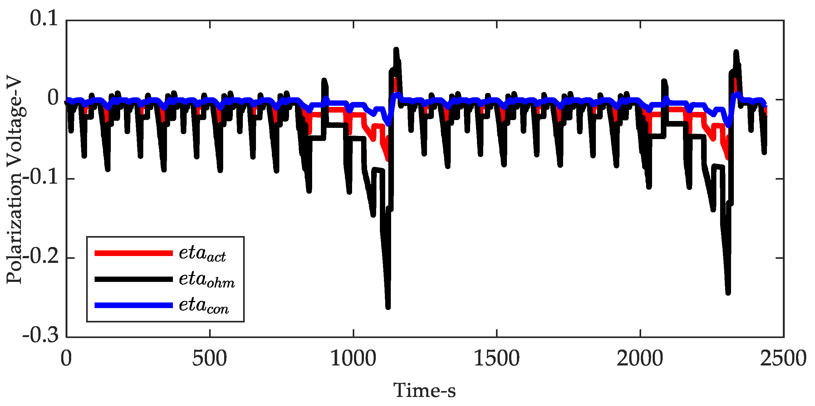
At an ambient temperature of 25 °C, the New European Driving Cycle (NEDC) data were used as the test data for real-time quantitative characterization of polarization voltage based on LDM. The data were fed into the characterization platform when SOC = 0.8468 and stopped when SOC = 0.7006. Input current update frequency and terminal voltage acquisition frequency were 1 Hz. The values of the model parameters at specific SOC level were obtained by interpolation of the previously calibrated curves. The current vs. terminal voltage curves (Figure 15), SOC curves (Figure 16), and polarization voltages (Figure 17) were plotted dynamically during cycling. Based on the hardware platform used, real-time characterization of polarization voltage drops at a frequency of 1 Hz could be achieved using the proposed method (actual calculation time consumption for each time step is less than 500 ms). The model output voltage maintained good tracking performance by comparing with the battery terminal voltage data obtained from the acquisition board. However, it was observed that the voltage tracking error increased when the current increased. The possible sources of error are (1) LDM does not include the electrolyte concentration polarization, (2) errors from the identification algorithm or the curve fitting, which are expected to be further improved. It can be seen that the voltage drop from all three types of polarization was positively correlated with the current applied to the cell, which is consistent with the findings of previous studies [14,17,49]. In summary, the proposed method achieves the function of quantitative characterization of polarization voltage, and the algorithm computation efficiency can meet a good real-time performance.
4. Conclusions
Based on LDM, this study characterizes all three types of polarization voltage of Lithium ion batteries under operating conditions. Three model parameters were used: dimensionless charge exchange current , ohmic resistance , and diffusion time constant to characterize activation polarization, ohmic polarization, and concentration polarization, respectively. A joint algorithm consisting of the PSO algorithm and the L-M method was used to identify the model parameters. The deviation of the model output terminal voltage from the actual terminal voltage was used as the accuracy criterion, and the proposed algorithm was compared with the PSO algorithm alone and the L-M method alone. In terms of the intercepted battery testing data, RMSE as the criterion, the voltage error of the joint algorithm was reduced 77.1% compared to the PSO algorithm only, and 72.3% compared to the L-M method only. To further test the effectiveness of the model and the identification algorithm, the identified model parameters were substituted into the second battery test data. It can be concluded that (1) the proposed scheme describes the nonlinear characteristics of the battery cell under the excitation of high dynamic driving conditions, (2) the model reflects the real physical-chemical processes inside the battery to a certain extent. To test the real-time performance of the proposed method, a hardware implementation platform for the real-time quantitative characterization of the polarization voltage of lithium-ion batteries was built, and the model parameters were calibrated and fitted using an offline method. The hardware platform was capable of realizing the basic function of quantitative polarization voltage characterization, and the update frequency of relevant parameters was 1 Hz, with good real-time performance. It has the potential for further development for BMS applications.
Author Contributions
B.X. and B.Y. proposed the novel method of polarization voltage characterization for lithium-ion batteries; B.Y. designed the experiment scheme and conducted experiments. B.Y. and J.C. designed and implemented the hardware platform; B.Y. wrote the paper. All authors have read and agreed to the published version of the manuscript.
Funding
This research was funded by National Natural Science Foundation of China (Grant No. 51877120).
Conflicts of Interest
The authors declare no conflict of interest.
Nomenclature
| Acronyms | |
| AC | Alternating current |
| BMS | Battery management system |
| CC-CV | Constant current Constant voltage |
| CCV | Closed-circuit voltage |
| DC | Direct current |
| DOP | Degree of Polarization |
| DRT | Distribution of Relaxation Times |
| GA | Genetic Algorithm |
| GITT | Galvanostatic intermittent titration technique |
| GS-EIS | Galvanostatic electrochemical impedance spectroscopy |
| LDM | Lumped diffusion model |
| L-M method | Levenberg-Marquardt method |
| Pseudo-2D | Pseudo 2 dimensional |
| PSO | Particle swarm optimization |
| PVDF | Ferroelectric polyvinylidene difluoride |
| QOCV | Quasi-open-circuit voltage |
| SOC | State of Charge |
| SOH | State of Health |
| SPM | Single particle model |
| Symbols | |
| Coefficients of polynomial describing SOC-OCV curve | |
| Local learning factor | |
| Global learning factor | |
| Randomly picked dimension among three dimensions | |
| Open-circuit voltage | |
| Battery terminal voltage | |
| Voltage error | |
| F | Faraday constant |
| Fitness function of PSO algorithm | |
| G | Maximum iteration number |
| , global optimum particle | |
| Applied current taken at 1C rate | |
| Applied current under discrete time domain | |
| Instantaneous current | |
| Local SOC in electrode particle | |
| Dimensionless charge exchange current | |
| Jacobian matrix | |
| Learning factor gain | |
| Maximum iteration number | |
| Current iteration number | |
| Lower velocity bound | |
| Lower position bound | |
| Identity matrix | |
| Dimension number of the particle | |
| , history optimum for the pth particle | |
| P | Population size |
| Battery capacity | |
| R | Molar gas constant |
| Ohmic resistance | |
| Random numbers uniformly distributed in (0,1) | |
| Average SOC of electrode particle | |
| Surface SOC of electrode particle | |
| SOC at initial time point | |
| Search space | |
| T | Reference temperature |
| Initial time | |
| Current time | |
| Upper velocity bound | |
| Upper position bound | |
| Model output voltage | |
| Real world terminal voltage | |
| , velocity vector for the pth particle | |
| , position vector for the pth particle | |
| Dimensionless space variable in particle size scale | |
| Greek symbols | |
| Charge transfer coefficient | |
| Tolerance | |
| Activation polarization overpotential | |
| Concentration polarization overpotential | |
| Ohmic polarization overpotential | |
| Parameter vector in the L-M method | |
| Diffusion time constant | |
| Maximum inertia weight | |
| Minimum inertia weight | |
| Inertia weight | |
| Subscripts/Superscripts | |
| Positive electrode | |
| Negative electrode | |
| The pth particle | |
| Iteration number | |
References
- Bizeray, A.M.; Kim, J.-H.; Duncan, S.R.; Howey, D.A. Identifiability and Parameter Estimation of the Single Particle Lithium-Ion Battery Model. IEEE Trans. Control Syst. Technol. 2019, 27, 1862–1877. [Google Scholar] [CrossRef] [Green Version]
- Xiaosong, H.; Li, S.; Peng, H. A Comparative Study of Equivalent Circuit Models for Li-Ion Batteries. J. Power Sources 2012, 198, 359–367. [Google Scholar]
- Junfu, L.; Wang, D.; Pecht, M. An Electrochemical Model for High C-Rate Conditions in Lithium-Ion Batteries. J. Power Sources 2019, 436, 226885. [Google Scholar]
- Shunli, W.; Stroe, D.; Fernandez, C.; Yu, C.; Zou, C.; Li, X. A Novel Energy Management Strategy for the Ternary Lithium Batteries Based on the Dynamic Equivalent Circuit Modeling and Differential Kalman Filtering under Time-Varying Conditions. J. Power Sources 2020, 450, 227652. [Google Scholar]
- Andreas, N.; Zavalis, T.G.; Elger, R.; Behm, M.; Lindbergh, G. Analysis of the Polarization in a Li-Ion Battery Cell by Numerical Simulations. J. Electrochem. Soc. 2010, 157, 11. [Google Scholar]
- Jiaxin, Z.; Lu, J.; Amine, K.; Pan, F. Depolarization Effect to Enhance the Performance of Lithium Ions Batteries. Nano Energy 2017, 33, 497–507. [Google Scholar]
- Changsheng, Q.; He, G.; Shi, W.; Zou, M.; Liu, C. The Polarization Characteristics of Lithium-Ion Batteries under Cyclic Charge and Discharge. J. Solid State Electrochem. 2019, 23, 1887–1902. [Google Scholar]
- Guanhua, F.; Li, Z.; Mi, L.; Zheng, J.; Feng, X.; Chen, W. Polypropylene/Hydrophobic-Silica-Aerogel-Composite Separator Induced Enhanced Safety and Low Polarization for Lithium-Ion Batteries. J. Power Sources 2018, 376, 177–183. [Google Scholar]
- Hyun-seung, K.; Kim, J.; Jang, J.; Kim, N.; Ryu, J.H.; Yoon, S.; Oh, S.M. A Comparative Study of Polarization During the Initial Lithiation Step in Tungsten-Oxide Negative Electrodes for Lithium-Ion Batteries. Solid State Ion. 2017, 311, 1–5. [Google Scholar]
- Ying, S.; Wen, L.; Li, F.; Cheng, H. Nanosized Li4ti5o12/Graphene Hybrid Materials with Low Polarization for high rate lithium ion Batteries. J. Power Sources 2011, 196, 8610–8617. [Google Scholar]
- Balasundaram, M.; Ramar, V.; Yap, C.; Balaya, P. Investigation of Physico-Chemical Processes in Lithium-Ion Batteries by Deconvolution of Electrochemical Impedance Spectra. J. Power Sources 2017, 361, 300–309. [Google Scholar]
- Woo-Jin, S.; Joo, S.H.; Kim, D.H.; Hwang, C.; Jung, G.Y.; Bae, S.; Son, Y.; Cho, J.; Song, H.; Kwak, S.K.; et al. Significance of Ferroelectric Polarization in Poly (Vinylidene Difluoride) Binder for High-Rate Li-Ion Diffusion. Nano Energy 2017, 32, 255–262. [Google Scholar]
- J, N.D.; Wang, M.; Le, A.V.; Shi, Y.; Qiao, Y. Internal Resistance and Polarization Dynamics of Lithium-Ion Batteries Upon Internal Shorting. Appl. Energy 2018, 212, 796–808. [Google Scholar]
- Yingxia, H.; Lai, H. Effects of Discharge Rate on Electrochemical and Thermal Characteristics of Lifepo4/Graphite Battery. Appl. Therm. Eng. 2019, 157, 113744. [Google Scholar]
- Noboru, S. Thermal Behavior Analysis of Lithium-Ion Batteries for Electric and Hybrid Vehicles. J. Power Sources 2001, 99, 70–77. [Google Scholar]
- Peyman, T.; Mansouri, A.; Yazdanpour, M.; Bahrami, M. Theoretical Analysis of Potential and Current Distributions in Planar Electrodes of Lithium-Ion Batteries. Electrochim. Acta 2014, 133, 197–208. [Google Scholar]
- Damian, G.; Faulkner, T.; Peterson, V.K.; Sharma, N. Structural Evidence for Mg-Doped Lifepo4 Electrode Polarisation in Commercial Li-Ion Batteries. J. Power Sources 2018, 394, 1–8. [Google Scholar]
- Haijun, R.; Jiang, J.; Sun, B.; Zhang, W.; Gao, W.; Wang, l.; Ma, Z. A Rapid Low-Temperature Internal Heating Strategy with Optimal Frequency Based on Constant Polarization Voltage for Lithium-Ion Batteries. Appl. Energy 2016, 177, 771–782. [Google Scholar]
- Xiaokang, L.; Wang, Q.; Yang, Y.; Kang, J. Correlation between Capacity Loss and Measurable Parameters of Lithium-Ion Batteries. Int. J. Electr. Power Energy Syst. 2019, 110, 819–826. [Google Scholar]
- Cyril, M.; Fullenwarth, J.; Monconduit, L.; Lestriez, B. Diagnostic of the Failure Mechanism in Nisb2 Electrode for Li Battery through Analysis of Its Polarization on Galvanostatic Cycling. Electrochim. Acta 2012, 78, 177–182. [Google Scholar]
- Bizhong, X.; Chen, G.; Zhou, J.; Yang, Y.; Huang, R.; Wang, W.; Lai, Y.; Wang, M.; Wang, H. Online Parameter Identification and Joint Estimation of the State of Charge and the State of Health of Lithium-Ion Batteries Considering the Degree of Polarization. Energies 2019, 12, 2939. [Google Scholar]
- Caiping, Z.; Jiang, J.; Gao, Y.; Zhang, W.; Liu, Q.; Hu, X. Polarization Based Charging Time and Temperature Rise Optimization for Lithium-Ion Batteries. Energy Procedia 2016, 88, 675–681. [Google Scholar]
- Zhang, C.; Jiang, J.; Gao, Y.; Zhang, W.; Liu, Q.; Hu, X. Charging Optimization in Lithium-Ion Batteries Based on Temperature Rise and Charge Time. Appl. Energy 2017, 194, 569–577. [Google Scholar] [CrossRef]
- Rong, X.; Yang, Y.; Yin, F.; Liu, P.; Cloetens, P.; Liu, Y.; Lin, F.; Zhao, K. Heterogeneous Damage in Li-Ion Batteries: Experimental Analysis and Theoretical Modeling. J. Mech. Phys. Solids 2019, 129, 160–183. [Google Scholar]
- Hosang, P.; Yoon, T.; Kim, Y.; Ryu, J.H.; Oh, S.M. Li2nio2 as a Sacrificing Positive Additive for Lithium-Ion Batteries. Electrochim. Acta 2013, 108, 591–595. [Google Scholar]
- Moya, A.A.; Castilla, J.; Horno, J. Ionic Transport in Electrochemical Cells Including Electrical Double-Layer Effects. A Network Thermodynamics Approach. J. Phys. Chem. 1995, 99, 1292–1298. [Google Scholar] [CrossRef]
- Bo, Y.; Lim, C.; Song, Z.; Zhu, L. Analysis of Polarization in Realistic Li Ion Battery Electrode Microstructure Using Numerical Simulation. Electrochim. Acta 2015, 185, 125–141. [Google Scholar]
- Junfu, L.; Wang, L.; Lyu, C.; Liu, E.; Xing, Y.; Pecht, M. A Parameter Estimation Method for a Simplified Electrochemical Model for Li-Ion Batteries. Electrochim. Acta 2018, 275, 50–58. [Google Scholar]
- Emil, N.; Torregrossa, D.; Cherkaoui, R.; Paolone, M. Parameter Identification of a Lithium-Ion Cell Single-Particle Model through Non-Invasive Testing. J. Energy Storage 2017, 12, 138–148. [Google Scholar]
- Thanh-Son, D.; Vyasarayani, C.P.; McPhee, J. Simplification and Order Reduction of Lithium-Ion Battery Model Based on Porous-Electrode Theory. J. Power Sources 2012, 198, 329–337. [Google Scholar]
- Xiaowei, Z.; Cai, Y.; Yang, L.; Deng, Z.; Qiang, J. State of Charge Estimation Based on a New Dual-Polarization-Resistance Model for Electric Vehicles. Energy 2017, 135, 40–52. [Google Scholar]
- Henrik, E.; Fridholm, B.; Lindbergh, G. Comparison of Lumped Diffusion Models for Voltage Prediction of a Lithium-Ion Battery Cell During Dynamic Loads. J. Power Sources 2018, 402, 296–300. [Google Scholar]
- Andre, D.; Meiler, M.; Steiner, K.; Wimmer, C.; Soczka-Guth, T.; Sauer, D.U. Characterization of High-Power Lithium-Ion Batteries by Electrochemical Impedance Spectroscopy. I. Experimental Investigation. J. Power Sources 2011, 196, 5334–5341. [Google Scholar] [CrossRef]
- Zhang, S.; Xu, K.; Jow, T. Electrochemical Impedance Study on the Low Temperature of Li-Ion Batteries. Electrochim. Acta 2004, 49, 1057–1061. [Google Scholar] [CrossRef]
- Moya, A.A. Identification of Characteristic Time Constants in the Initial Dynamic Response of Electric Double Layer Capacitors from High-Frequency Electrochemical Impedance. J. Power Sources 2018, 397, 124–133. [Google Scholar] [CrossRef]
- Xing, Z.; Huang, J.; Pan, Z.; Ouyang, M. Impedance Characterization of Lithium-Ion Batteries Aging under High-Temperature Cycling: Importance of Electrolyte-Phase Diffusion. J. Power Sources 2019, 426, 216–222. [Google Scholar]
- Santhanagopalan, S.; Guo, Q.; Ramadass, P.; White, R.E. White. Review of Models for Predicting the Cycling Performance of Lithium Ion Batteries. J. Power Sources 2006, 156, 620–628. [Google Scholar] [CrossRef]
- Doyle, M.; Fuller, T.F.; Newman, J. Modeling of Galvanostatic Charge and Discharge of the Lithium/Polymer/Insertion Cell. J. Electrochem. Soc. 1993, 140, 1526–1533. [Google Scholar] [CrossRef]
- Srinivasan, V.; Wang, C.Y. Analysis of Electrochemical and Thermal Behavior of Li-Ion Cells. J. Electrochem. Soc. 2003, 150, A98. [Google Scholar] [CrossRef] [Green Version]
- Botte, G.G.; Subramanian, V.R.; White, R.E. White. Mathematical Modeling of Secondary Lithium Batteries. Electrochim. Acta 2000, 45, 2595–2609. [Google Scholar] [CrossRef]
- Haran, B.S.; Popov, B.N.; White, R.E. White. Determination of the Hydrogen Diffusion Coefficient in Metal Hydrides by Impedance Spectroscopy. J. Power Sources 1998, 75, 56–63. [Google Scholar] [CrossRef]
- Diwakar, V.D. Towards Efficient Models for Lithium Ion Batteries. Ph.D. Thesis, Tennessee Technological University, Ann Arbor, MI, USA, 2009. [Google Scholar]
- Shen, W.-J.; Li, H.-X. Parameter Identification for the Electrochemical Model of Li-Ion Battery. In Proceedings of the 2016 International Conference on System Science and Engineering (ICSSE), Puli, Taiwan, 7–9 July 2016. [Google Scholar]
- Kennedy, J.; Eberhart, R. Particle Swarm Optimization. In Proceedings of the ICNN’95—International Conference on Neural Networks, Perth, WA, Australia, 27 November–1 December 1995. [Google Scholar]
- Levenberg, K. A Method for the Solution of Certain Non-Linear Problems in Least Squares. Q. Appl. Math. 1944, 2, 164–168. [Google Scholar] [CrossRef] [Green Version]
- Marquardt, D.W. An Algorithm for Least-Squares Estimation of Nonlinear Parameters. J. Soc. Ind. Appl. Math. 1963, 11, 431–441. [Google Scholar] [CrossRef]
- Lyshevski, S.E. Engineering and Scientific Computations Using Matlab; John Wiley & Sons: Hoboken, NJ, USA, 2005. [Google Scholar]
- Bizhong, X.; Huang, R.; Lao, Z.; Zhang, R.; Lai, Y.; Zheng, W.; Wang, H.; Wang, W.; Wang, M. Online Parameter Identification of Lithium-Ion Batteries Using a Novel Multiple Forgetting Factor Recursive Least Square Algorithm. Energies 2018, 11, 11. [Google Scholar]
- Myounggu, P.; Zhang, X.; Chung, M.; Less, G.B.; Sastry, A.M. A Review of Conduction Phenomena in Li-Ion Batteries. J. Power Sources 2010, 195, 7904–7929. [Google Scholar]
Figure 1.
Major steps of the joint parameter identification algorithm.

Figure 2.
Outline of the test bench: offline calibration and schedule condition application.
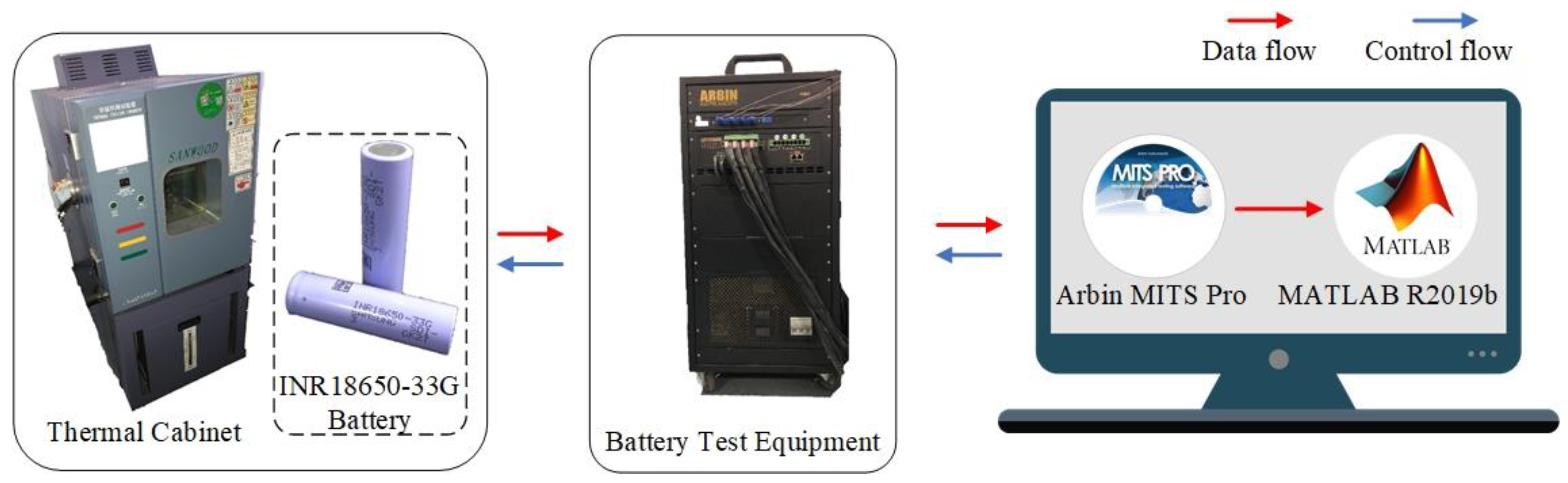
Figure 3.
Outline of the hardware platform: online characterization of polarization voltage.
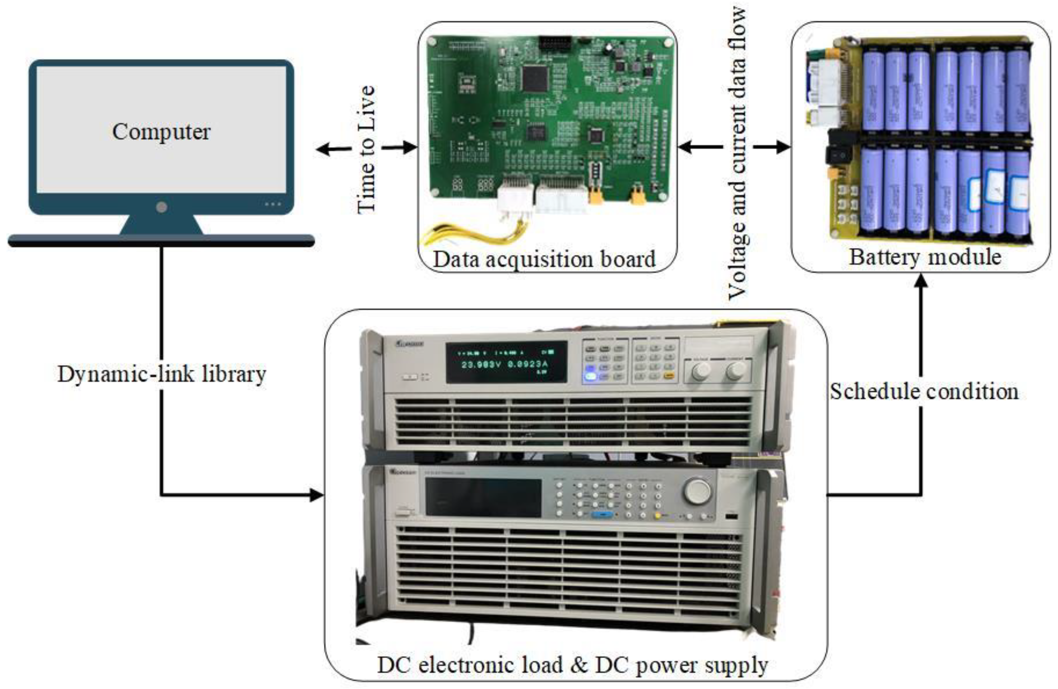
Figure 4.
Schedule of experiments.

Figure 5.
The measured data points and fitted curve of SOC versus OCV.
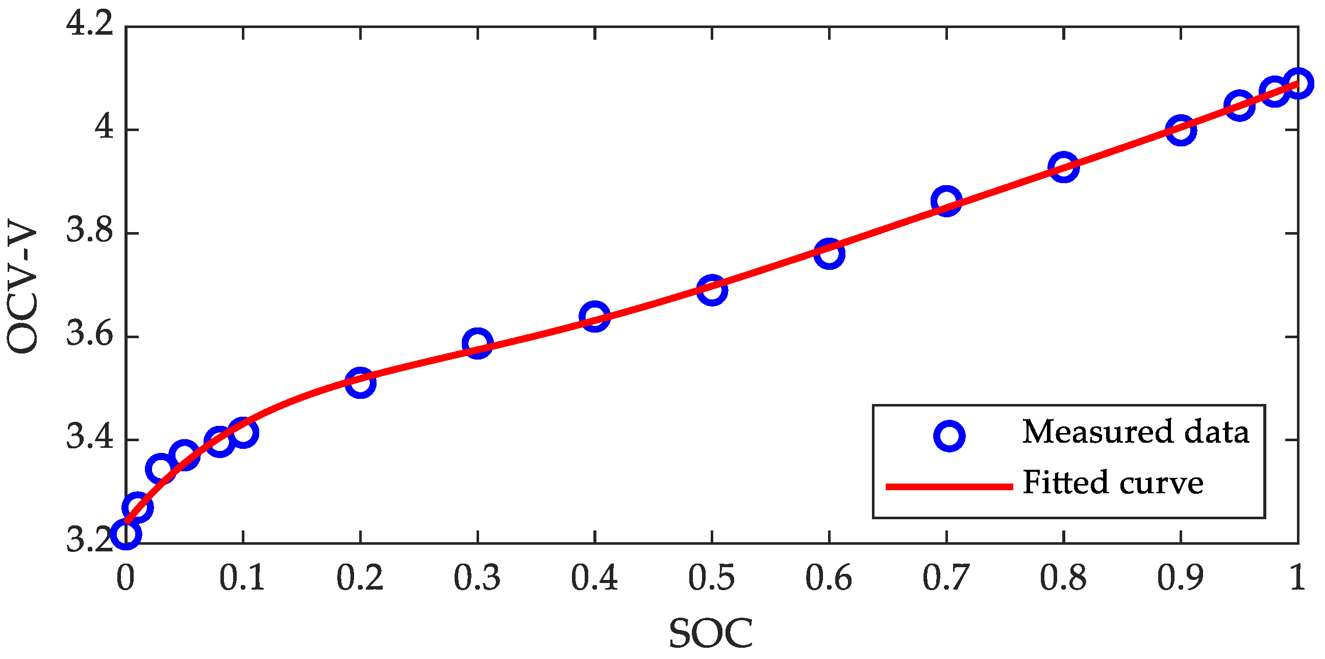
Figure 6.
Current profile of the CITY operating condition test.

Figure 7.
Comparison of LDM output voltage curve based on three types of parameter identification algorithm during the CITY test at 25 °C ambient temperature. (a) Voltage curve; (b)voltage error curve.
Figure 7.
Comparison of LDM output voltage curve based on three types of parameter identification algorithm during the CITY test at 25 °C ambient temperature. (a) Voltage curve; (b)voltage error curve.
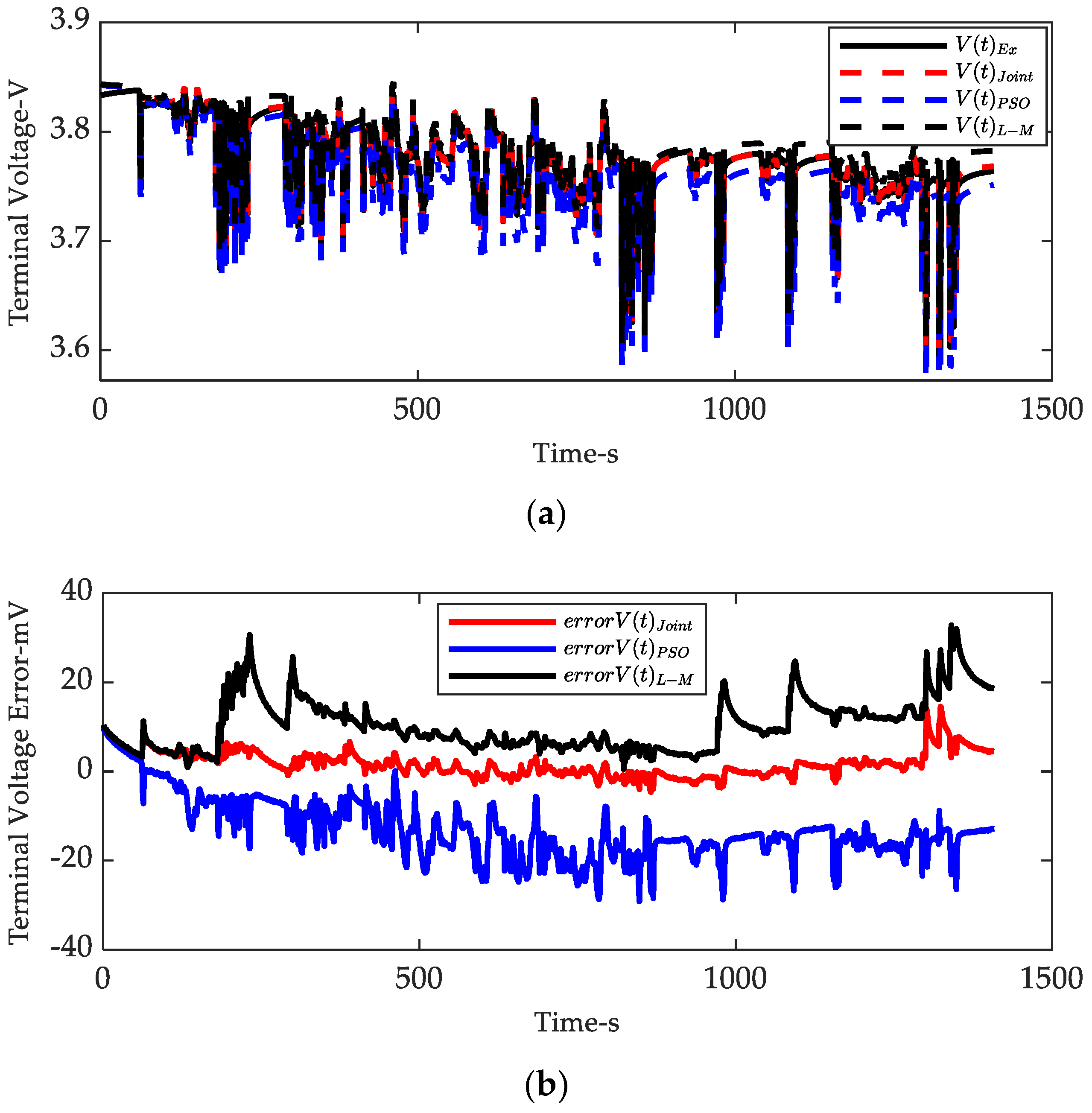
Figure 8.
Model output voltage error curve based on the second group of testing data.
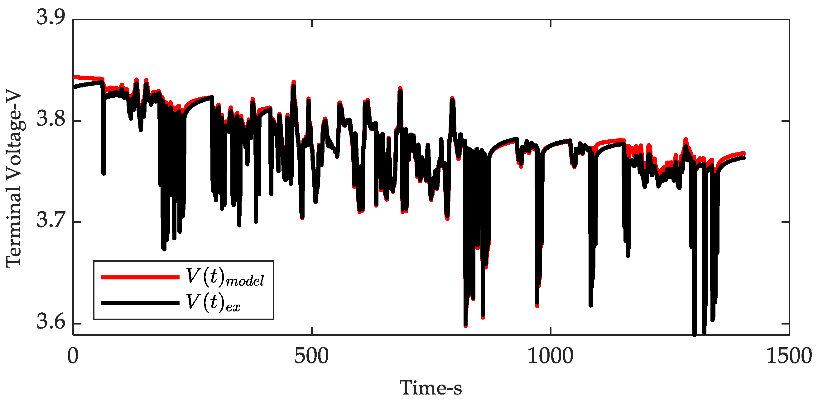
Figure 9.
Temporal and spatial distribution of iSOC inside the electrode particle during the CITY test at 25 °C ambient temperature.
Figure 9.
Temporal and spatial distribution of iSOC inside the electrode particle during the CITY test at 25 °C ambient temperature.

Figure 10.
Variation curve of SOC on the surface of electrode particles with time.
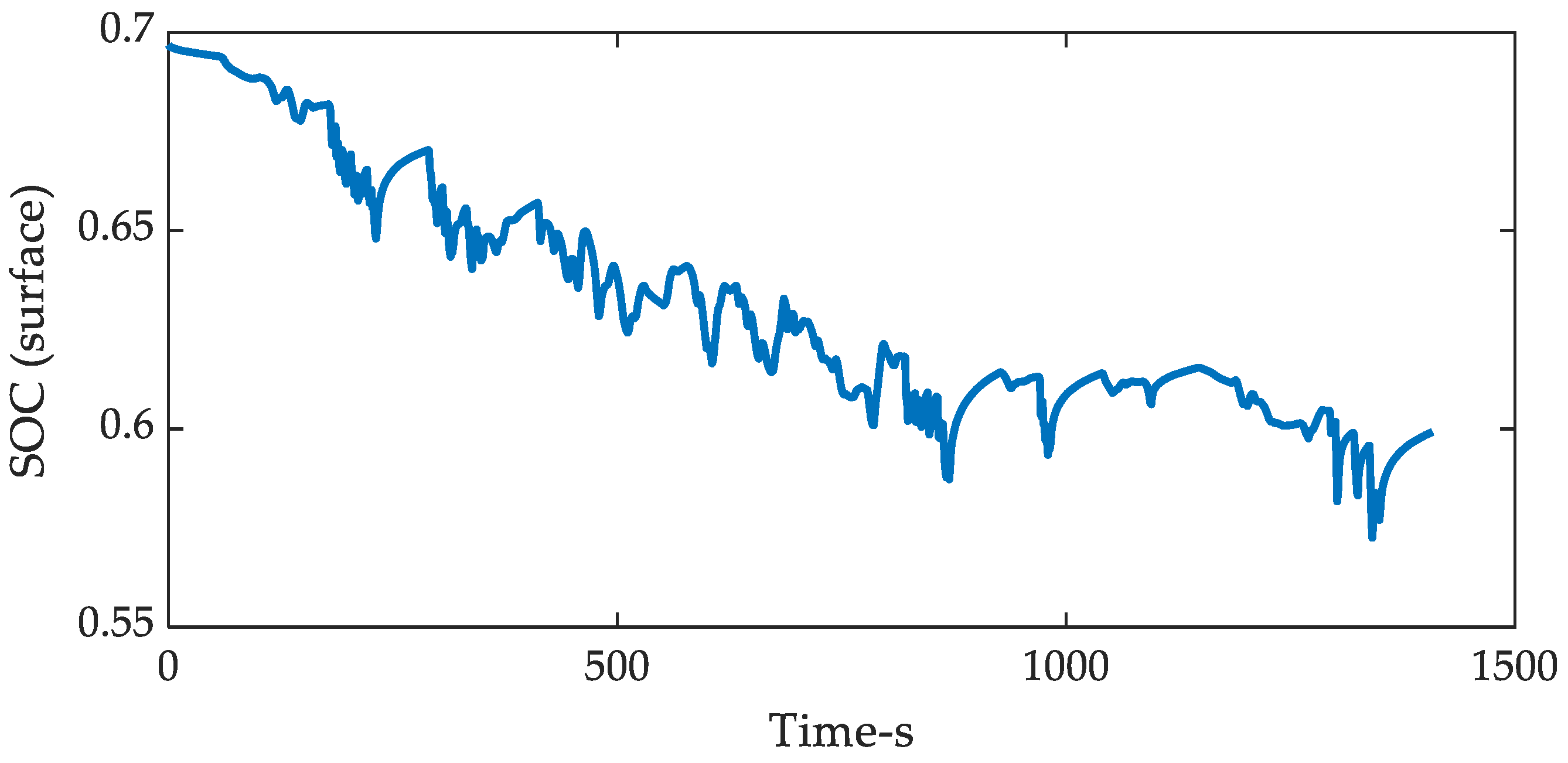
Figure 11.
Quantitative characterization curves of three types of polarization voltage based on LDM.
Figure 11.
Quantitative characterization curves of three types of polarization voltage based on LDM.
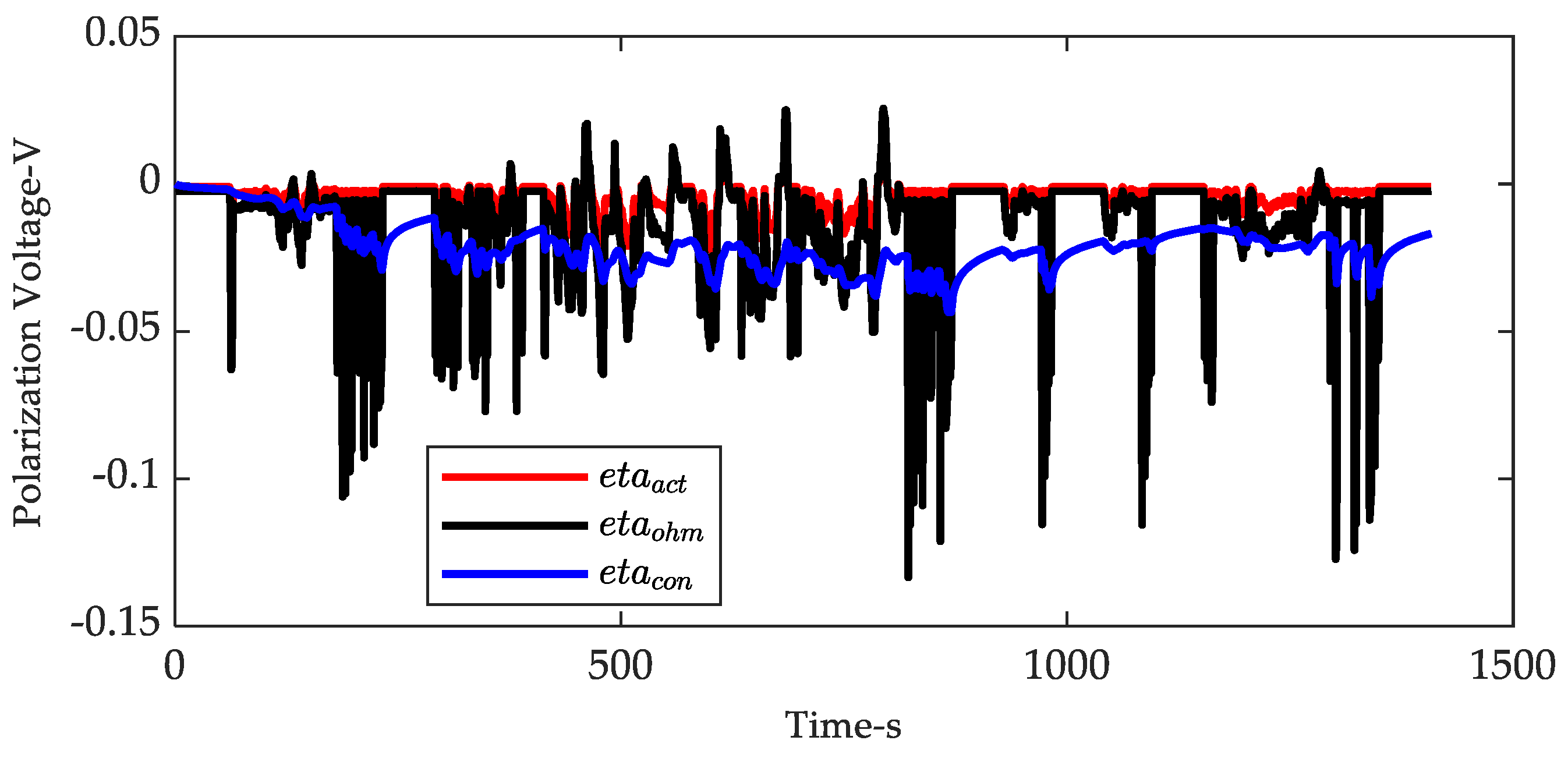
Figure 12.
Variation curve of diffusion time constant with SOC.
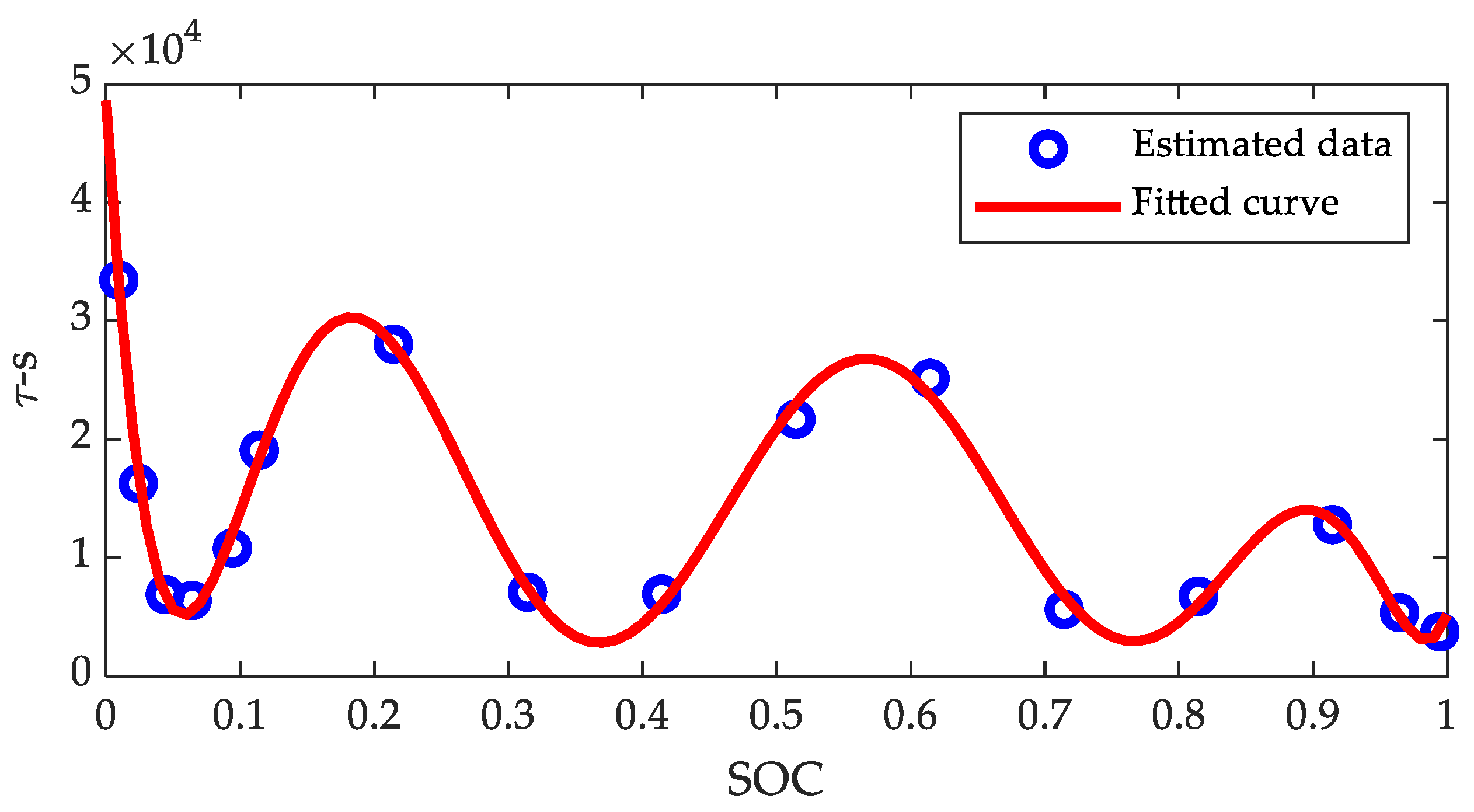
Figure 13.
Variation curve of dimensionless charge exchange current with SOC.
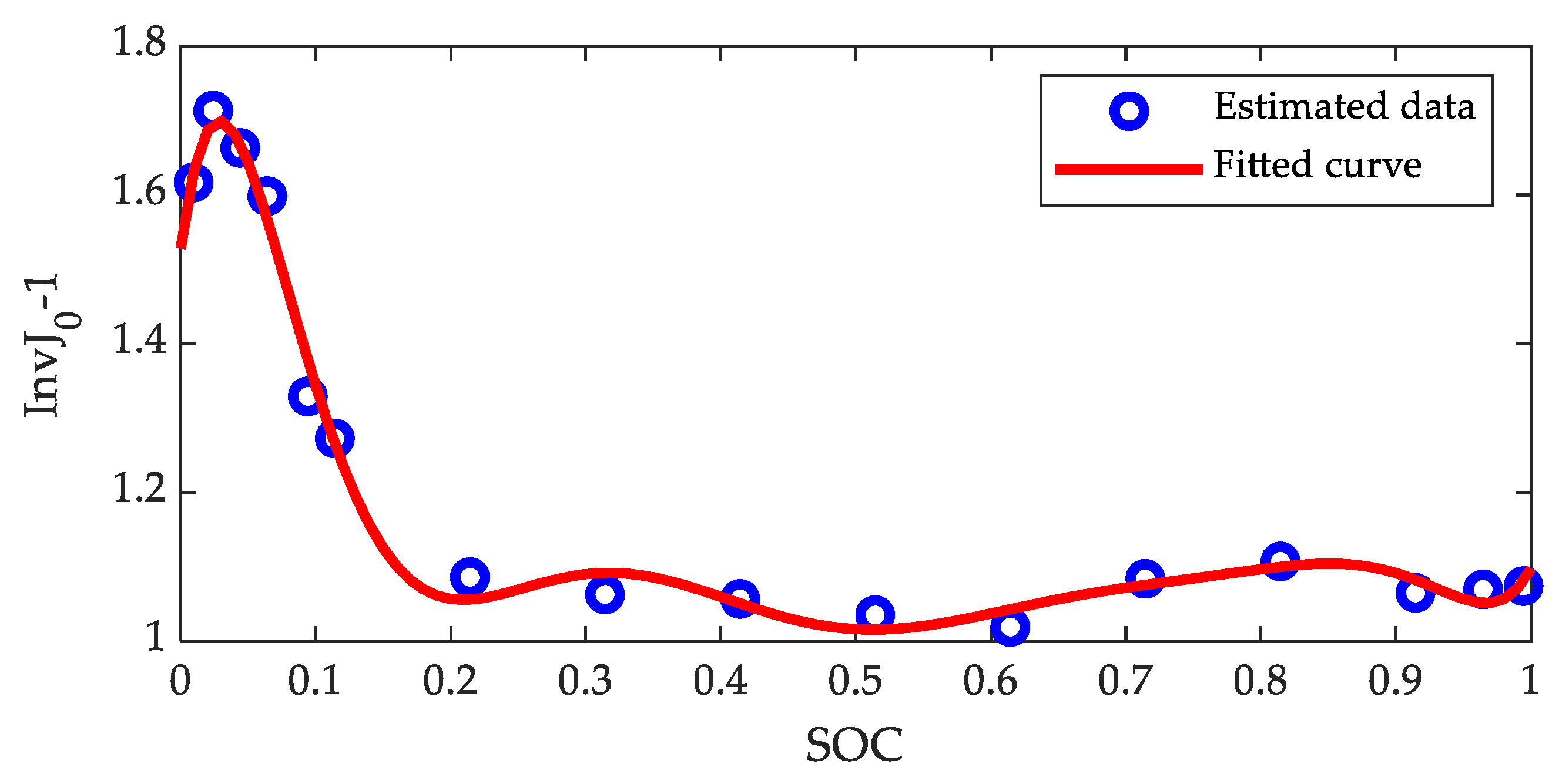
Figure 14.
Variation curve of ohmic overpotential at 1 C rate with SOC.

Figure 15.
Accuracy test of hardware implementation platform under NEDC schedule at 25 °C ambient temperature. (a) NEDC current profile. (b) Comparison of model output voltage and actual voltage.
Figure 15.
Accuracy test of hardware implementation platform under NEDC schedule at 25 °C ambient temperature. (a) NEDC current profile. (b) Comparison of model output voltage and actual voltage.
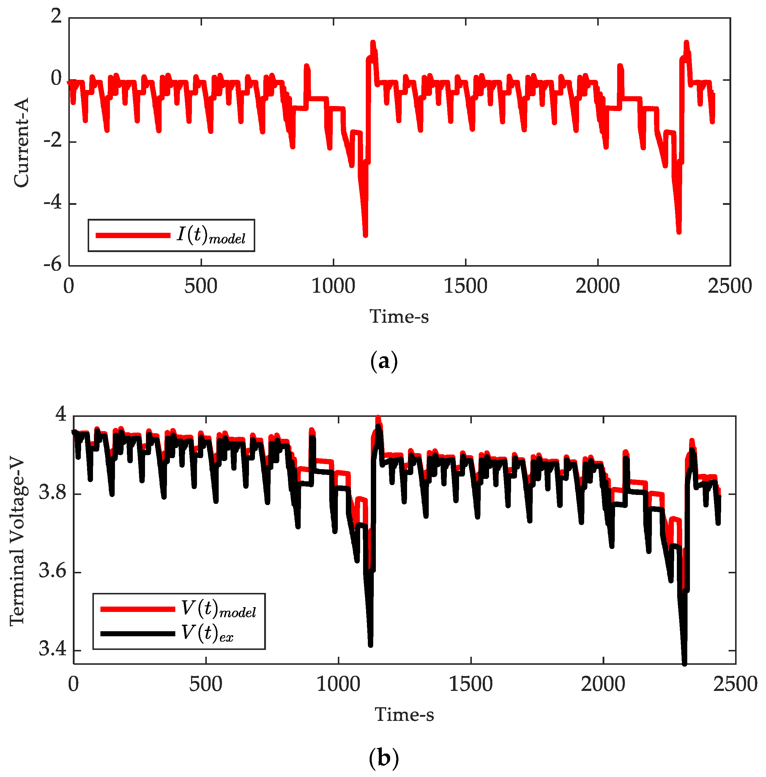
Figure 16.
SOC curve based on ampere-hour integral method under the NEDC condition.
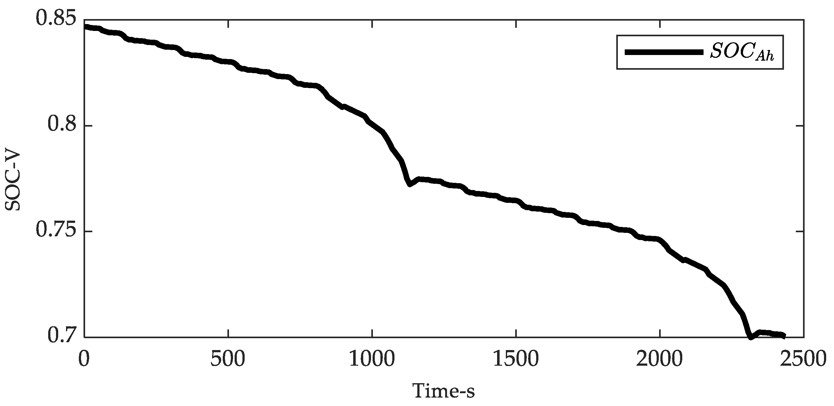
Figure 17.
Curves of three kinds of polarization voltage under the NEDC condition.

Table 1.
Polynomial coefficients of SOC-OCV curve.
| Coefficients | |||||||
|---|---|---|---|---|---|---|---|
| Values | −5.0010 | 20.8142 | −34.1273 | 27.8136 | −11.4670 | 2.8176 | 3.2400 |
Table 2.
Model parameter identification results of three types of algorithm.
| Algorithm | (Dimensionless) | /mV | |
|---|---|---|---|
| PSO Algorithm | 17,447 | 2.6007 | 49.279 |
| L-M Method | 10,163 | 1.0765 | 69.642 |
| Joint Estimation Algorithm | 10,034 | 1.1412 | 69.62 |
Table 3.
Voltage error statistics based on model parameters from three algorithms.
| Algorithm | PSO Algorithm | L-M Method | Joint Estimation Algorithm |
|---|---|---|---|
| Mean Voltage Error/V | 0.0128780611 | 0.0104785487 | 0.0017621340 |
| Voltage RMSE/V | 0.0145556022 | 0.0120200028 | 0.0033290570 |
Publisher’s Note: MDPI stays neutral with regard to jurisdictional claims in published maps and institutional affiliations. |
© 2022 by the authors. Licensee MDPI, Basel, Switzerland. This article is an open access article distributed under the terms and conditions of the Creative Commons Attribution (CC BY) license (https://creativecommons.org/licenses/by/4.0/).
Share and Cite
MDPI and ACS Style
Xia, B.; Ye, B.; Cao, J. Polarization Voltage Characterization of Lithium-Ion Batteries Based on a Lumped Diffusion Model and Joint Parameter Estimation Algorithm. Energies 2022, 15, 1150. https://doi.org/10.3390/en15031150
AMA Style
Xia B, Ye B, Cao J. Polarization Voltage Characterization of Lithium-Ion Batteries Based on a Lumped Diffusion Model and Joint Parameter Estimation Algorithm. Energies. 2022; 15(3):1150. https://doi.org/10.3390/en15031150
Chicago/Turabian StyleXia, Bizhong, Bo Ye, and Jianwen Cao. 2022. "Polarization Voltage Characterization of Lithium-Ion Batteries Based on a Lumped Diffusion Model and Joint Parameter Estimation Algorithm" Energies 15, no. 3: 1150. https://doi.org/10.3390/en15031150
Note that from the first issue of 2016, this journal uses article numbers instead of page numbers. See further details here.