
Computational Model of Shell and Finned Tube Latent Thermal Energy Storage Developed as a New TRNSYS Type


Faculty of Engineering, University of Rijeka, Vukovarska 58, 51000 Rijeka, Croatia
*
Author to whom correspondence should be addressed.
Energies 2022, 15(7), 2434; https://doi.org/10.3390/en15072434
Submission received: 16 February 2022
/
Revised: 22 March 2022
/
Accepted: 23 March 2022
/
Published: 25 March 2022
(This article belongs to the Section D: Energy Storage and Application)
Abstract
:This paper presents the development of a computational model of latent thermal energy storage (LTES) in a shell and tube configuration with longitudinal fins. The model describes the physical process of transient heat transfer between the heat transfer fluid (HTF) and the phase change material (PCM) in LTES. For modeling the phase change of the PCM, the enthalpy formulation was used. Based on a one-dimensional computational model, a new Trnsys type was developed and written in Fortran. Validation of the LTES model was performed by comparing numerically and experimentally obtained data for the melting and solidification of paraffin RT 25 as the PCM and water as the HTF. Numerical investigations of the effect of HTF inlet temperature and HTF flow rate on heat transfer in LTES confirmed that significant improvement in heat transfer between the HTF and PCM could be achieved by increasing the HTF inlet temperature during charging or decreasing the HTF inlet temperature during discharging. Increasing the HTF flow rate did not significantly improve the heat transfer between the HTF and PCM, both during charging and discharging. The presented, experimentally validated LTES model could be used to analyze the feasibility of integrating LTES into various thermal systems and ultimately help define the specific benefits of implementing LTES systems.
1. Introduction
With the goal of protecting the environment and preserving favorable climate conditions, efforts have been made globally in recent decades to reduce greenhouse gas emissions, increase energy efficiency, and increase the share of renewable energy. The residential sector accounts for about 26.1% of final energy consumption in the EU, the largest share of which is energy for space heating (63.6%) and domestic hot water production (14.8%) [1]. This suggests that improving energy consumption in the residential sector has great potential to reduce greenhouse gas emissions, increase energy efficiency, and increase the share of renewable energy. Energy from renewable sources accounts for 21.1% of total energy consumption for residential heating in the EU, and with a share of 1.9%, the feasibility of solar thermal has yet to be proven [1]. Since solar energy is only available during the day, when heating demand is lower, and is not available in the late evening and at night, when heating demand is higher, the time mismatch between solar energy availability and heating demand must be overcome through the use of thermal energy storage. Traditionally, sensible thermal energy storage (STES) systems using water as the storage medium have been used due to their low investment cost [2]. However, due to their advantages over sensible thermal energy storage systems—higher energy storage density, ability to store energy at a constant temperature, and lower heat losses—latent thermal energy storage (LTES) systems are of particular interest for use in thermal systems with heat pumps because they can potentially increase heat pump efficiency [3,4].
Experimental research on heat pump systems with LTES in the available literature mostly has been performed using multiple measurements over several days with different ambient conditions and operating strategies [5,6,7,8,9,10]. Numerical research on heat pump systems with LTES in the literature has been performed using various dynamic system simulation software that allow modeling of the mutual interaction of thermal systems and heating loads under transient boundary conditions [11,12,13,14,15,16]. The application of dynamic simulation facilitates seasonal analyses of thermal systems, since the research times are shorter and the costs are lower compared to the costs of experimental research. The introduction of dynamic simulation of thermal systems can provide comprehensive results that can lead to a better understanding of system operation under unsteady boundary conditions and working parameters [17].
In LTES, heat is stored or released during phase change of the phase change material (PCM) used as the heat storage medium. Thermal energy generated by the heat pump or received from solar collectors can be delivered to LTES by a heat transfer fluid (HTF) and stored in the PCM by melting. The motivation for using LTES is that the stored energy can be used for directly supplying consumers, which can increase the share of renewable energy, or to provide a heat source at a suitable temperature for the heat pump, which can increase its efficiency. The physical problem of heat transfer in LTES consists of forced flow convection on the HTF side, and heat conduction through the tubes and heat transfer on the PCM side of LTES. In liquid PCMs, heat transfer can be augmented by natural convection—buoyancy-induced motion caused by density variations in liquid PCMs [18]. Due to its complexity, the problem of heat transfer during phase change of the PCM is usually analyzed numerically using computational fluid dynamics [19,20]. In this way, both heat transfer and fluid flows are modeled by applying conservation of mass, momentum, and energy. Since these models can be computationally extensive and time consuming, their application in dynamic system simulations is limited. For this reason, a common approach to modeling LTES for use in dynamic system simulations is to simplify the mathematical model. Various approaches can be found in the literature.
Leonhardt et al. [21] modeled LTES with an encapsulated PCM using Modelica software. The model was designed such that the PCM was encapsulated in plate structures and surrounded by water. Thermal resistance through the walls of the plates was neglected. The authors used a modified heat capacity approach to model the phase change of the PCM.
Feng et al. [22] modeled LTES in a shell and tube configuration for use in Trnsys. The HTF flowed through the tube and the PCM filled the space around the tube. The heat transfer effect of the HTF and PCM in the axial direction has been neglected. The modeling of heat transfer during phase changes has been approached using the enthalpy method. The authors compared the HTF outlet temperatures, average PCM temperatures, and liquid fractions obtained with the model in Trnsys to those obtained with a numerical model in the CFD software Fluent. The comparison was presented for both melting and solidification. The authors analyzed the influence of HTF inlet temperature and HTF flow rate on the average PCM temperature and HTF outlet temperature and concluded that the influence of HTF inlet temperature is superior to that of HTF flow rate.
Another model of shell and tube LTES was developed by Cunha et al. [12], who considered multiple passes of the HTF through LTES. The model was created in Matlab. The authors considered the temperature dependent PCM thermal conductivity and volumetric heat capacity. The effect of natural convection during PCM melting was accounted for by the equivalent thermal conductivity. The validation of the mathematical model and numerical method was performed by comparing the numerically and experimentally determined average PCM temperatures, HTF outlet temperatures and heat transfer rates for both melting and solidification processes.
Belmonte et al. [23] proposed a simplified bypass factor method for modeling LTES suitable for use in simulations of thermal systems. The model was created in Matlab, but the simulations were performed in Trnsys through the use of the Type 155 subroutine. The bypass factor method assumes splitting the HTF flow at the LTES inlet in two currents—one current flowing through an ideal LTES where the thermal resistances between the HTF and PCM are neglected, and the other current being fully bypassed to the LTES outlet. The value of the bypass factor that best fits the thermal response of a model to experimental tests was calibrated separately for organic and inorganic PCMs using GenOpt software. The proposed model was validated by comparing the HTF outlet temperature, heat rate, and stored heat between the experimental and numerical results for both organic and inorganic PCM melting and solidification processes. The authors stated that the model is suitable for dynamic modeling of thermal systems, especially in the early stages of thermal system design.
Heinz et al. [24] developed a one-dimensional LTES model in Fortran for use in Trnsys. In the LTES, the PCM was encapsulated in plates, spheres, or cylinders and surrounded by water as the HTF. The LTES model was divided height-wise into isothermal segments, where for each segment heat transfer between the HTF and the PCM is described by the energy balance equation. Convection on the PCM side was not considered. The enthalpy approach was used to model heat transfer during the phase change of the PCM. The model allows simulation of various PCMs, but the temperature-dependent thermal properties of the PCM must be provided by the user in an appropriate ASCII data file. The LTES model was validated against experimental measurements in terms of HTF outlet temperatures, PCM temperatures, and heat transfer rates.
Helmns et al. [25] developed and validated a dimensionless first-principles LTES model for use in Modelica. The authors modeled a LTES with an inorganic PCM, encapsulated in rectangular modules with HTF flowing around them. The validation was performed by comparing HTF outlet temperatures, accumulated energy, and heat transfer rates with experimental data for melting and solidification processes.
Gowreesunker et al. [26] coupled Trnsys and Fluent in order to model the thermal performance of a PCM plate heat exchanger. To simulate the thermal performance of the PCM heat exchanger under dynamic boundary conditions, the model in Fluent was coupled with Trnsys via a script and results file. At each time step, Trnsys transmitted input data to Fluent and received the output from the Fluent model. To model the heat transfer between the PCM and air, the authors used a two-dimensional CFD model based on the enthalpy method.
A literature review showed that experimentally validated LTES models suitable for use in dynamic thermal system simulations are not widely available, potentially hindering research on thermal systems that utilize LTES. Because the dominant thermal resistance in LTES is on the PCM side, due to low thermal conductivity of PCMs, finned tubes have been considered in an effort to achieve better heat transfer between the HTF and the PCM by increasing the heat transfer surface and reducing the heat transfer resistance on the PCM side. The motivation for this is to analyze the energy efficiency and feasibility of thermal systems utilizing LTES with increased heat transfer surface and lower thermal resistance on the PCM side. There has not been found any research on modeling of a LTES tank in a shell and tube configuration with longitudinal fins suitable for use in dynamic thermal system simulations. With the goal of advancing thermal system modeling using heat pumps and LTES, this paper presents the development of a time-effective and accurate mathematical model of LTES in a shell-and-tube configuration with longitudinal fins, suitable for use in dynamic thermal system simulations. Both the melting and solidification processes were numerically analyzed and the results were compared with experimental data obtained by measurements on an experimental LTES to validate the developed LTES model. The Trnsys subroutine was written in Fortran, and a new component—Type 2021—was created that can be used in simulations of thermal systems. Using the developed LTES model, the effects of various operating parameters on the thermal performance of LTES were investigated and presented.
2. Physical Problem
The physical problem involves heat transfer between the HTF and the PCM inside LTES in a shell and finned tube configuration with longitudinal fins. Heat is delivered or collected by the HTF flowing through the tubes while the PCM fills the LTES shell. Heat transfer between the HTF and PCM occurs by convective heat transfer within the tubes, conduction through the walls of the tubes and fins and convection and conduction on the PCM side of the LTES. Since heat can be stored or released during phase change of the PCM, both latent and sensible heat can be used. During a charging process, the delivered heat can be used to heat the solidified PCM, melt the PCM and heat the molten PCM. Heat for charging the LTES in domestic heating systems can be provided by solar thermal collectors or by a heat pump to store the excess heat during periods of lower heating demand. Once stored, the heat can either be used to supply consumers directly, typically using PCMs with a melting temperature above 40 °C [11,12,16,21], or as a high-temperature heat source for the heat pump, typically using PCMs with a melting temperature below 30 °C [5,10,14]. In this study, the melting temperature of the PCM was 25 °C.
A 3D schematic representation of the analyzed shell and finned tube LTES model is given in Figure 1, and the technical drawing of the section of the analyzed LTES is given in Figure 2.
The LTES shown in Figure 1 and Figure 2 is a shell and tube tank with longitudinal fins in which the HTF flows through the tubes while the PCM fills the shell space around the fins and tubes. The HTF enters at the top and exits at the bottom. The outer shell of the tank is made of stainless steel and insulated with a 25 mm thick foam rubber layer, while both the fins and the tubes are made of aluminum. The values of the geometry parameters of the LTES are given in Table 1 and the thermophysical properties of the LTES materials and PCM are given in Table 2. The PCM is an organic paraffin—Rubytherm RT 25. Each tube has eight angularly equidistant fins. Because of the low thermal conductivity of organic PCMs, dominant thermal resistance in LTES is on the PCM side [27,28]. The purpose of using fins is an effort to achieve better heat transfer between the HTF and the PCM by increasing the heat transfer area and thus reducing the heat transfer resistance on the PCM side. Heat transfer between the HTF and the PCM occurs by convection from the HTF to the inner tube wall, conduction through the walls of tubes and fins, and convection and conduction on the PCM side. During heating or cooling of a solidified PCM, conduction is the only means of heat transfer through the PCM. However, heat transfer in liquid PCM can be augmented by natural convection.
3. Computational Model
The computational model is a one-dimensional multi-node model describing the transient heat transfer between the HTF and PCM in a shell and finned tube LTES. PCM and HTF temperatures are numerically calculated at the end of each time step based on the energy conservation equation as well as initial and boundary conditions. The effect of natural convection on the PCM side is included along with that of conduction in a liquid PCM [18,29,30,31]. The following assumptions were considered: the PCM is homogeneous and isotropic [21,22,26], the physical properties of the HTF, tubes and fins are constant [21,22,23,24,25,26], and the HTF flow is laminar. Natural convection effects in a liquid PCM are included through an equivalent thermal conductivity coefficient [32,33,34]. LTES is divided into isothermal segments in the HTF flow direction [24]. The thermal resistance through the fins is included through fin efficiency [25].
Figure 3 shows a schematic representation of the computational LTES tank model with multiple nodes, and the ith segment with calculated heat fluxes, which form the energy conservation equation for the segment.
The PCM and HTF subdomains are divided into an equal number of segments in the HTF flow direction. The PCM segments are isothermal, whereas the change in temperature over a segment was accounted for in HTF segments. The ith segment shown in Figure 3 thermally interacts with the neighboring upper and lower segments, the HTF and the environment. The energy conservation equation for the ith segment is defined as follows:
In Equation (1) [kg] is the PCM mass in the ith segment, Hi [J/kgK] is PCM specific enthalpy in ith segment, t [s] is time, [W] is exchanged heat flux with the HTF, [W] is exchanged heat flux with neighboring upper segment, [W] is exchanged heat flux with neighboring lower segment and [W] are ith segment thermal losses through the outer wall of LTES. Equation (1) can further be written as:
where UAhx,i [W/K] is the reciprocal value of the total heat transfer resistance between HTF and PCM, ∆Tm,i [K] is the mean logarithmic temperature difference between HTF temperature at inlet and outlet of tube ith segment and PCM temperature in the ith segment, kPCM [W/mK] is PCM thermal conductivity, AIF [m2] is interface area between neighboring segments, δx [m] is height of the ith segment, TPCM,i−1, TPCM,i and TPCM,i+1 [K] are PCM temperatures at segments i − 1, i and i + 1, Uloss [W/m2K] is the total heat transfer coefficient between PCM and environment, As,i [m2] is the area of ith segment to environment and Tenv [K] is environment temperature.
Modeling of the phase change of the PCM is approached with the enthalpy formulation [35,36], in which specific enthalpy is a function of the temperature defined as follows:
The specific enthalpy H [J/kg] given in Equation (3) consists of the sensible specific enthalpy and the specific enthalpy change during phase change of the PCM. In Equation (3) l [J/kg] is the latent heat of the PCM, cPCM [kJ/kgK] is the PCM specific heat capacity and γ [-] is the liquid fraction defined as:
In Equation (4), Tsolidus and Tliquidus are the temperatures at which the phase change begins or ends, depending on whether the charging or discharging process is occurring i.e., whether heat is being stored or released from the PCM. During the charging process, the PCM in the ith segment is in the solid state when its temperature is lower than Tsolidus; it consists of both solid and liquid phases when its temperature is Tsolidus < TPCM,i < Tliquidus and it is liquid when its temperature is higher than Tliquidus.
Various organic PCMs with low melting temperatures achieve a non-isothermal melting process, i.e., a small temperature rise occurs during melting, while solidification is isothermal [32,37,38,39,40]. Since an organic PCM with a low melting temperature, paraffin RT25, was used in this study, it achieved isothermal solidification, and Tsolidus and Tliquidus were the same for the LTES discharge.
Figure 4 shows the top view of the longitudinally finned tube and the surrounding PCM annulus, and the selected section shows a schematic representation of the thermal resistances that occur between the HTF and PCM. Based on this schematic representation, the equation for UAhx is derived as the reciprocal of the total thermal resistance between the HTF and PCM, which is given in Equation (5).
In Figure 4 and in Equation (5) R1, R2, R3 and R4 represent thermal resistances due to convection heat transfer on the inside of tubes, conductive heat transfer through the tube wall, heat transfer from outside of the tube to the PCM and heat transfer from the fins to the PCM, respectively, as given in Equations (6)–(9).
In Equations (6)–(9) hHTF [W/m2K] denotes the convective heat transfer coefficient inside the tubes, Ain [m2] is the inside area of the tube, do and di [m] are the outside and inside tube diameters, Li [m] is tube and fin length in the ith segment, kt [W/mK] is tube thermal conductivity, DPCM [m] is the diameter of a PCM subdomain, which, considering all tubes are equidistant, is equal to the tube pitch, kPCM [W/mK] is PCM thermal conductivity, δPCM [m] is average PCM thickness between two adjacent fins, Af,i [m2] is fin area and ηf [-] is fin efficiency.
Thermal resistance due to conductive heat transfer through fins is included through fin efficiency [25], which is defined as:
where b [-] is calculated as
In Equation (11) kf [W/mK] and tf [m] denote thermal conductivity of the fin and the fin thickness respectively. The convective heat transfer on the HTF side is defined by the Gnielinski correlation [41,42,43]:
In Equation (12), kHTF is thermal conductivity of the HTF, Re and Pr are Reynolds and Prandtl numbers given as:
In Equations (13) and (14), ρHTF [kg/m3] is HTF density, μHTF [Pa s] is HTF dynamic viscosity, cHTF [J/kgK] is HTF specific heat capacity and uHTF [m/s] is HTF inlet velocity.
The effects of natural convection in liquid PCM are included through the equivalent thermal conductivity coefficient [32,33,34], as given in Equation (15):
where C and n are coefficients, values of which are 0.05 and 0.25 respectively [32,33], kPCM [W/mK] is thermal conductivity of the PCM and Ra is the Rayleigh number:
In Equation (16), g [m/s2] denotes gravitational acceleration, β [1/K] denotes the thermal expansion coefficient, THTF,in [K] is HTF inlet temperature, TPCM,m [K] is melting temperature of the PCM, νPCM [m2/s] is kinematic viscosity of the PCM and aPCM [m2/s] is thermal diffusivity of the PCM.
4. Numerical Procedure and Experimental Validation
4.1. Numerical Setup
The numerical procedure for obtaining temperature and enthalpy distributions of the PCM was based on the finite volume method [44]; however, only energy conservation was considered. By doing so, the physical problem of heat transfer in LTES was simplified to reduce computational time while maintaining the required accuracy of the results, making the model more suitable for using within dynamic thermal system simulations. The computational domain, i.e., the LTES tank, was divided into isothermal segments (finite volumes) and the partial differential equation (1) was discretized into a system of algebraic equations over the LTES segments. The system of algebraic equations was solved and temperature and enthalpy distributions of the PCM were obtained. In order to calculate the PCM enthalpy change in any segment over a time step, the terms on the right-hand side in Equation (1) representing the heat fluxes at segment boundaries needed to be known. The HTF outlet temperatures of each time step were obtained using the values of PCM temperatures from the previous time step.
The computational code was written in Fortran and compiled for use in Trnsys, a widely used software for transient system simulations. The inputs read at the beginning of each time step were HTF inlet temperature, HTF flow rate and ambient temperature, while the parameters read at the start of the simulation and remaining constant throughout the simulation were LTES tank geometry parameters, PCM mass, physical properties of the PCM, HTF and heat exchanger materials as well as liquidus and solidus temperatures for both melting and solidification.
4.2. Independency Analysis of Number of Segments and Time Step Size
Computational time and accuracy are important issues in dynamic thermal system simulations. In order to ensure the numerical results were independent of the number of segments into which the LTES tank was divided, numerically obtained PCM temperature profiles in the PCM segment positioned at the middle axial position of the LTES were compared for 31, 35, 39 and 41 segments for a melting process with HTF mass flow 620 l/h and inlet temperature 37 °C (Figure 5). The initial temperature of the PCM was 15 °C.
It can be observed in Figure 5 that in the case of a smaller considered number of segments, the melting time is slightly longer. Since no significant difference in PCM transient temperature profiles was observed for numbers of segments 39 and 41, solution independence from the number of segments was confirmed and in further analyses, the LTES tank was divided into 39 isothermal segments to save the computational time and also maintain the accuracy of results.
Time step sizes can range from 10 s to 15 min in dynamic thermal systems simulations, and even longer if building simulation tools are integrated [45,46]. In order to save on computational time and ensure that the results were time step independent, time step size independence analysis was performed. Simulations were carried out using time step sizes 30 s, 1 min, 2 min and 5 min and the results were compared in terms of transient temperature profiles in the PCM segment positioned at the middle axial position of the LTES (Figure 6).
As shown in Figure 6, there is no significant difference between PCM transient temperature profiles obtained numerically with time step sizes 30 s and 1 min, which confirms the independence of the results from time step size. Upon analyzing the independence of results from the number of isothermal segments into which the LTES tank is divided and time step size, the division of the LTES tank model into 39 segments and a time step size of 1 min were selected and used in further analyses.
4.3. Experimental Validation
In order to validate the developed LTES model, experimental measurements on LTES with Rubitherm RT25 paraffin as the PCM were performed in the Laboratory for Thermal Measurements of the Faculty of Engineering, University of Rijeka. The experimental setup consists of an LTES tank, cold and hot HTF supply, a control valve, a circulation pump, an automatic control system to ensure a constant HTF mass flow and inlet temperature at the LTES inlet, temperature sensors and a flow meter. The schematic representation of the experimental setup is shown in Figure 7 and the experimental LTES tank is shown in Figure 8.
The test system can operate in one of two modes: charge mode, when hot HTF is provided by the heat pump condenser, and discharge mode, when the heat pump evaporator provides cold HTF to the tank. A constant HTF inlet temperature was ensured by the three-way control valve, continuously adjusted by the automatic control system.
Type K thermocouples were used to measure the HTF and PCM temperatures. The thermocouples were placed at the LTES inlet and outlet (T1 and T2) to measure the HTF inlet and outlet temperatures. For the measurement of PCM temperatures, a set of thermocouples was installed at axial positions 0.2 m, 0.75 m and 1.3 m away from the HTF inlet in the LTES tank (T3, T4 and T5). The HTF volumetric flow rate was measured using the ultrasonic flowmeter (FM). The thermocouples and the flow meter were connected to a personal computer via a data acquisition system. An application was created in Labview and used for acquiring, processing and storing measured values. The application provided real-time monitoring of the measured temperatures and flow rate.
The measurements were performed during both melting and solidification, and transient variations of HTF and PCM temperatures were obtained. Numerical dynamic simulations of the melting and solidification processes were performed and the validation of the proposed computational model and numerical procedure was performed by comparing the results of the numerical dynamic simulations with the measured data. The numerical results were compared with the experimentally obtained data in terms of PCM temperatures, HTF outlet temperatures and accumulated/released energy. The HTF temperatures at the LTES inlet were 42 °C for melting and 7 °C for solidification and the HTF flow rate was 620 l/h. The initial temperatures of the PCM at the beginning of the simulations in the entire LTES tank were 13 °C for melting and 35 °C for solidification.
Numerically obtained HTF outlet temperatures (position T2) and PCM temperatures at axial positions 0.2 m (position T3), 0.75 m (position T4), and 1.3 m (position T5) are shown in Figure 9 and compared with experimental data for melting. Positions T2, T3, T4, and T5, for which the numerically obtained temperatures are shown in Figure 9, correspond to positions where the water and paraffin temperatures were measured during the experiments. The comparison of the experimentally and numerically obtained accumulated energy is shown in Figure 10. The experimentally obtained accumulated and released energies in each time interval were calculated as the product of HTF mass flow rate, HTF specific heat capacity, temperature difference at the inlet and outlet of the LTES tank and the time interval in which the data were measured and recorded.
It can be observed in Figure 9 that the transient profiles of HTF outlet temperature obtained with the computational model are in good agreement with experimentally measured HTF temperatures during the entire melting process. The overall discrepancy between predicted and measured HTF outlet temperatures was 1.29%. Overall discrepancies between predicted and measured PCM temperatures at positions T3, T4 and T5 were 3.29%, 6.45% and 4.04% respectively. Melting was completed first at position T3, followed by T4 and T5, which can be observed by the accentuated rise in temperature profiles after reaching the melting temperature of 25 °C.
The comparison shown in Figure 10 indicates good agreement between the numerically obtained accumulated energy and the accumulated energy calculated from experimental data throughout the entire considered period. The overall discrepancy was 5.75% and the relative error at 14 h was less than 1% between the numerically and experimentally obtained accumulated energy.
Numerical results of HTF outlet temperature, PCM temperature and released energy during solidification were compared to the experimental data and presented in Figure 11 and Figure 12.
In Figure 11, the similarity between the predicted and experimental HTF outlet transient temperature variations and PCM temperatures can be observed, suggesting a good agreement between the numerical results and experimental data. The overall discrepancy between predicted and measured HTF outlet temperature throughout the 16 h period was 7.59%. Overall discrepancies between predicted and measured PCM temperatures at positions T3, T4 and T5 were 9.86%, 1.42% and 2.33% respectively. The temperature profile representing position T3 is the first to drop below the melting temperature of 25 °C, indicating that the PCM is first solidified in the upper part of the tank, closest to the HTF inlet, followed by the PCM in segments at positions T4 and T5.
The comparison of released energy is presented in Figure 12. The overall discrepancy between predicted released energy and calculated released energy using experimental data was 8.88% whereas the relative error at 16 h was 5.36% between numerically and experimentally obtained accumulated energy.
5. Application of the Developed Model
With the aim to demonstrate the applicability of the developed LTES model in Trnsys, the thermal performance of the LTES was numerically investigated under various operating conditions. A series of numerical simulations was performed with different HTF inlet temperatures and flow rates. The impact of different HTF inlet temperatures and HTF flow rates on LTES thermal performance was analyzed through comparison of transient variations of PCM temperatures, accumulated/released energy and mean heat transfer rates. The results are presented and discussed for both charging and discharging processes. The accumulated/released energy at the end of each time step was calculated as the sum of accumulated/released energies in all previous time steps and the mean heat transfer rate during LTES charging/discharging was calculated by dividing accumulated/released energy by charging/discharging time.
5.1. The Influence of HTF Inlet Temperature
5.1.1. Influence of HTF Inlet Temperature on LTES Thermal Performance during Charging
Transient variations of PCM temperatures obtained by the numerical model during LTES charging for HTF inlet temperatures 35 °C, 40 °C and 45 °C are presented in Figure 13, and the comparison of accumulated energy obtained by the numerical model during LTES charging is presented in Figure 14 for the same HTF inlet temperatures. The HTF flow rate was 800 l/h and initial PCM temperature was 15 °C in all analyzed cases.
The LTES charging process shown in Figure 13 can be divided into three stages. During the first stage, the PCM is in a solid state. This stage can be identified by an accentuated rise in the PCM temperature at the beginning of the charging process due to storing only sensible heat. In the second stage, a slow and uniform rise of PCM temperature can be observed. This is due to storing both sensible and latent heat during melting. In the third stage, the PCM is completely melted and its temperature rises more quickly again due to only storing sensible heat and finally reaches the final temperature for the given boundary conditions.
The developed LTES model confirmed a significant impact of HTF inlet temperature on LTES thermal performance during melting, which can be observed from the mismatch in transient variations of PCM temperature shown in Figure 13. The shortest melting time was achieved for the highest considered HTF inlet temperature of 45 °C, which indicates a more intense heat transfer between the HTF and PCM when the difference between the HTF inlet temperature and PCM temperature is greater. The difference among PCM temperature profiles shown in Figure 13 is more emphasized after the melting had already begun and even more towards the end of melting, showing the impact of HTF inlet temperature on the LTES charging process, while it is less prominent at the beginning of the charging process. When the PCM had completely melted, its temperature increased towards the HTF inlet temperature.
Regarding the accumulated energy, the highest accumulated energy was achieved for the highest HTF inlet temperature, as shown in Figure 14. This is because the LTES heat capacity is proportional to the temperature difference between the HTF and the PCM. After approximately 15 h, no significant increase in accumulated energy can be observed for the HTF inlet temperature of 45 °C. This can be explained by the fact that there is a finite amount of energy that can be stored in a PCM within a given temperature range, after which no extra energy can be stored. The accumulated energy for HTF inlet temperature 45 °C at 15 h was 169.4 MJ, while for HTF inlet temperature of 35 °C, the accumulated energy at 15 h was 136.15 MJ. The calculated relative difference between accumulated energy at 15 h for HTF inlet temperatures of 35 °C and 45 °C was 24.42%, suggesting that the impact of HTF inlet temperature on heat transfer in LTES during charging is significant. Similar to what has been observed for PCM temperatures, the difference among accumulated energy is more emphasized towards the end of the charging process.
The comparison of mean heat transfer rates during LTES charging is shown in Figure 15. Since for the highest considered HTF inlet temperature of 45 °C, no significant increase in accumulated energy can be observed after 15 h, the mean heat transfer rates for all considered HTF inlet temperatures were calculated for a time period of 15 h.
As shown in Figure 15, the highest mean heat transfer rate during charging was achieved for the highest considered HTF inlet temperature, which agrees with the previously presented results. By increasing the HTF inlet temperature from 35 °C to 45 °C, a 26.7% higher mean heat transfer rate can be achieved.
5.1.2. Influence of HTF Inlet Temperature on LTES Thermal Performance during Discharging
Transient variations of PCM temperatures obtained by the numerical model during discharging for HTF inlet temperatures of 5 °C, 10 °C and 15 °C are presented in Figure 16, and the comparison of released energy obtained by the numerical model during LTES discharging is presented in Figure 17 for the same considered HTF inlet temperatures. The HTF flow rate was 800 l/h and initial PCM temperature was 35 °C in all cases.
The discharging process shown in Figure 15 can be divided into three stages. During the first stage, the PCM is liquid, releasing only sensible heat, which can be observed by the decreasing trend in PCM temperatures at the beginning of the discharging process. In the second stage, the solidification occurs—the PCM releases heat but remains at a constant temperature, which is common for organic PCMs [32,37,38,39,40]. This is due to releasing only latent heat during solidification. In the third stage, the PCM is completely solid; its temperature decreases again due to releasing sensible heat.
From transient variations of PCM temperatures shown in Figure 15, it can be observed that the shortest solidification time was achieved for the lowest considered HTF inlet temperature of 5 °C, which indicates a more intense heat transfer between the HTF and the PCM when the difference between the HTF inlet temperature and PCM temperature is greater.
In Figure 17, it can be observed that the highest released energy was achieved for the lowest considered HTF inlet temperature of 5 °C. The total released energy at the end of the simulation at 24 h for an HTF inlet temperature of 5 °C was 167.5 MJ while for an HTF inlet temperature of 15 °C, the total released energy at the end of the simulation was 151.2 MJ.
The mean heat transfer rates calculated for different HTF inlet temperatures were compared for a discharging time period of 24 h and the comparison is shown in Figure 18.
From the comparison of mean heat transfer rates given in Figure 18, it can be seen that the highest mean heat transfer rate during discharging was achieved for the lowest considered HTF inlet temperature, i.e., when the temperature difference between the HTF and the PCM was the greatest. By decreasing the HTF inlet temperature from 15 °C to 5 °C, a 33.8% higher mean heat transfer rate can be achieved.
5.2. The Influence of HTF Flow Rate
The influence of different HTF flow rates on LTES thermal performance is discussed for charging and discharging processes.
5.2.1. Influence of HTF Flow Rate on LTES Thermal Performance during Charging
Transient variations of temperature in PCM segments at the exact middle of the LTES in the axial direction obtained by the numerical model during LTES charging for HTF flow rates 700 l/h, 800 l/h and 900 l/h are presented in Figure 19, and the comparison of accumulated energy obtained by numerical model during LTES charging for the same HTF flow rates is presented in Figure 20. The HTF inlet temperature during charging was 40 °C and initial PCM temperature was 15 °C in all considered cases.
No significant difference among the presented transient variations of PCM temperature can be observed in Figure 19, which indicates that for the considered range of HTF flow rates, the impact of different HTF flow rates on heat transfer in LTES during charging is minimal.
The similarity among the appearances of transient profiles of accumulated energy shown in Figure 20 suggests that the impact of different HTF flow rates on accumulated energy during charging is not as significant as the impact of different HTF inlet temperatures. The greatest relative difference between accumulated energies throughout the simulation obtained for the lowest and highest considered HTF flow rates, 700 l/h and 900 l/h, was 4.45%.
The mean heat transfer rates obtained for different HTF flow rates is shown in Figure 21.
The mean heat transfer rates during charging process for HTF flow rates 700 l/h, 800 l/h and 900 l/h were 2.98 kW, 3.02 kW and 3.06 kW respectively. The relative difference between mean heat transfer rates calculated for HTF flow rates 700 l/h and 900 l/h was 2.68% which confirms that the impact of HTF flow rate on heat transfer during the LTES charging process for the considered operating conditions is insignificant compared to the impact of HTF inlet temperature.
5.2.2. Influence of HTF Flow Rate on LTES Thermal Performance during Discharging
Transient variations of temperature in PCM segment at the exact middle of the LTES in the axial direction obtained by the numerical model for LTES discharging and for HTF flow rates 700 l/h, 800 l/h and 900 l/h are presented in Figure 22. The comparison of released energy obtained by the numerical model during LTES discharging is presented in Figure 23 for the same HTF flow rates. The HTF inlet temperature during discharging was 10 °C and the initial PCM temperature was 35 °C in all considered cases.
No significant difference among the transient variations of PCM temperature shown in Figure 22 can be observed. Slight differences among the presented transient variations of PCM temperatures can be seen after the solidification ended. The dashed line representing HTF flow rate of 900 l/s is the first to drop below 25 °C, indicating that the solidification completed sooner than in the cases of 700 l/s and 800 l/s HTF flow rates. Compared to the impact of different HTF inlet temperatures on PCM temperature, the impact of different HTF flow rates is insignificant for the considered range of HTF flow rates during discharging.
The comparison of released energy shown in Figure 23 suggests that the impact of different HTF flow rates on released energy during discharging is not as significant as the impact of different HTF inlet temperatures. The greatest calculated relative difference between released energies obtained for the lowest and highest considered HTF flow rates of 700 l/h and 900 l/h was 3.16%.
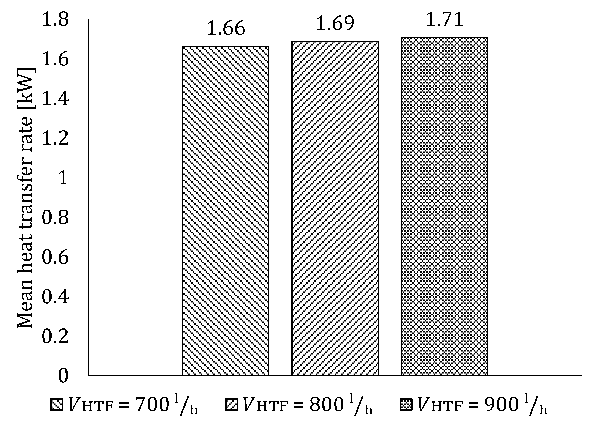
The mean heat transfer rates obtained for different HTF flow rates during LTES discharging are shown in Figure 24.
As can be seen in Figure 24, the mean heat transfer rates during the discharging process for HTF flow rates of 700 l/h, 800 l/h and 900 l/h were 1.66 kW, 1.69 kW and 1.71 kW, respectively. The relative difference between mean heat transfer rates obtained for HTF flow rates of 700 l/h and 900 l/h was 3.01%, which indicates that compared to the impact of HTF inlet temperature on heat transfer between the HTF and PCM during the LTES discharging process for the considered operating conditions, the impact of HTF flow rate is insignificant.
6. Conclusions
A computational model of LTES describing heat transfer between the HTF and PCM in a shell and tube configuration tank with longitudinal fins was developed and the numerical procedure was presented. The results independence from the number of segments into which the model is divided and from the time step size were examined, whereupon melting and solidification processes were numerically analyzed. The computational model and the numerical procedure were successfully validated against experimental data obtained by performing measurements on an experimental LTES.
To demonstrate the applicability of the model in Trnsys, the influence of HTF inlet temperatures and HTF flow rates on heat transfer between the HTF and PCM was investigated for both charging and discharging processes. It was shown that by increasing the HTF inlet temperature from 35 °C to 45 °C during LTES charging, 26.7% higher mean heat transfer rate can be achieved, while by decreasing the HTF inlet temperature from 15 °C to 5 °C during LTES discharging, 33.8% higher mean heat transfer rate can be achieved. Regarding the influence of HTF flow rate on heat transfer, it was shown that increasing the HTF flow rate from 700 l/h to 900 l/h can result in 2.68% higher mean heat transfer during charging and 3.01% higher mean heat transfer during discharging. Thus, it was confirmed that the impact of HTF inlet temperature on heat transfer during both charging and discharging processes is significant. The higher the temperature difference between the HTF and PCM, the more intense the heat transfer between the HTF and PCM could be achieved. Regarding the HTF flow rate, no significant improvement in heat transfer was observed when the HTF flow rate was increased, suggesting that the impact of HTF flow rate on heat transfer in LTES is negligible compared to the impact of HTF inlet temperature.
The developed, experimentally validated LTES computational model and numerical procedure are suitable for application to dynamic thermal systems simulations. The model can be used in the early stages of system design to analyze the feasibility of integrating LTES in various thermal systems and ultimately aid in improving the efficiency and sustainability of thermal systems.
Author Contributions
Conceptualization, F.T., K.L. and A.T.; methodology, F.T., K.L. and A.T.; software, F.T.; validation, F.T., K.L. and A.T.; formal analysis, F.T., K.L. and A.T.; investigation, F.T., K.L. and A.T.; resources, K.L. and A.T.; data curation, F.T.; writing—original draft preparation, F.T.; writing—review and editing, F.T., K.L. and A.T.; visualization, F.T., K.L. and A.T.; supervision, K.L. and A.T.; project administration, A.T.; funding acquisition, A.T. All authors have read and agreed to the published version of the manuscript.
Funding
Croatian Science Foundation: IP-2016-06-4095; University of Rijeka: uniri-tehnic-18-69.
Institutional Review Board Statement
Not applicable.
Informed Consent Statement
Not applicable.
Data Availability Statement
Not applicable.
Acknowledgments
This work was supported in part by the Croatian Science Foundation under the project HEXENER (IP-2016-06-4095) and in part by the University of Rijeka under the project number “uniri-tehnic-18-69”.
Conflicts of Interest
The authors declare no conflict of interest.
Nomenclature
| Af | Fin area in the ith segment (m2) |
| Ahx,i | Heat transfer area between HTF and PCM in the ith segment (m2) |
| AIF | Interface area between neighboring segments (m2) |
| Ain | Inside tube heat transfer area (m2) |
| As,i | Area of the ith segment to environment (m2) |
| a | Thermal diffusivity (m2/s) |
| B | Fin width (m) |
| b | Coefficient (-) |
| C | Coefficient (-) |
| c | Specific heat capacity (J/kgK) |
| D | LTES tank inside diameter (m) |
| di | Tube inside diameter (m) |
| do | Tube outside diameter (m) |
| ft | Fin thickness (m) |
| g | Gravitational acceleration (m/s2) |
| H | Specific enthalpy (J/kg) |
| h | Convective heat transfer coefficient (W/m2K) |
| k | Thermal conductivity coefficient (W/mK) |
| keq | Equivalent thermal conductivity coefficient (W/mK) |
| L | Fin length & LTES tank height (m) |
| l | Latent heat (J/kg) |
| Mass flow of the HTF (kg/s) | |
| mPCM,i | Mass of the PCM in ith segment (kg) |
| n | Coefficient (-) |
| nf | Number of fins per tube (-) |
| nt | Number of tubes (-) |
| Pr | Prandtl number (-) |
| Exchanged heat flux (W) | |
| Thermal losses through the LTES outer wall (W) | |
| R1 | Thermal resistance on the inside of the tubes (K/W) |
| R2 | Thermal resistance through tube wall (K/W) |
| R3 | Thermal resistance on the outside of the tubes (K/W) |
| R4 | Thermal resistance on the fin surface (K/W) |
| Ra | Rayleigh number (-) |
| Re | Reynolds number (-) |
| T | Temperature (K) |
| Tm | Melting temperature (K) |
| t | Time (s) |
| tp | Tube pitch (m) |
| U | Total heat transfer coefficient (W/m2K) |
| uHTF | HTF inlet velocity (m/s) |
| Greek symbols | |
| β | Thermal expansion coefficient (1/K) |
| γ | Liquid fraction (-) |
| ΔTm | Mean logarithmic temperature difference (K) |
| δPCM | Average PCM thickness between two adjacent fins (m) |
| δx | Height of the ith segment (m) |
| ηf | Fin efficiency (-) |
| μ | Dynamic viscosity (Pa s) |
| ν | Kinematic viscosity (m2/s) |
| ρ | Density (kg/m3) |
| Subscripts | |
| env | Environment |
| HTF | Heat transfer fluid |
| i | ith segment |
| in | Inlet |
| liquidus | PCM liquidus temperature |
| loss | Thermal losses to the environment |
| n | Number of LTES segments |
| out | Outlet |
| PCM | Phase change material |
| solidus | PCM solidus temperature |
| t | Tube |
References
- European Commission. EU Energy in Figures—Statistical Pocketbook; Publications Office of the European Union: Luxembourg, 2020. [Google Scholar] [CrossRef]
- Osterman, E.; Stritih, U. Review on compression heat pump systems with latent thermal energy storage for heating and cooling of buildings. J. Energy Storage 2021, 39, 102569. [Google Scholar] [CrossRef]
- Pardiñas, A.A.; Justo Alonso, M.; Diz, R.; Husevåg Kvalsvik, K.; Fernández-Seara, J. State-of-the-art for the use of phase-change materials in tanks coupled with heat pumps. Energy Build. 2017, 140, 28–41. [Google Scholar] [CrossRef] [Green Version]
- Kapsalis, V.; Karamanis, D. Solar thermal energy storage and heat pumps with phase change materials. Appl. Therm. Eng. 2016, 99, 1212–1224. [Google Scholar] [CrossRef]
- Comakli, O.; Kaygusuz, K.; Ayhan, T. Solar-assisted heat pump and energy storage for residential heating. Sol. Energy 1993, 51, 357–366. [Google Scholar] [CrossRef]
- Minglu, Q.; Liang, X.; Deng, S.; Yiqiang, J. Improved indoor thermal comfort during defrost with a novel reverse-cycle defrosting method for air source heat pumps. Build. Environ. 2010, 45, 2354–2361. [Google Scholar] [CrossRef]
- Long, J.Y.; Zhu, D.S. Numerical and experimental study on heat pump water heater with PCM for thermal storage. Energy Build. 2008, 40, 666–672. [Google Scholar] [CrossRef]
- Agyenim, F.; Hewitt, N. Experimental investigation and improvement in heat transfer of paraffin PCM RT58 storage system to take advantage of low peak tariff rates for heat pump applications. Int. J. Low-Carbon Technol. 2013, 8, 260–270. [Google Scholar] [CrossRef]
- Chen, H.; Wang, Y.; Li, J.; Cai, B.; Zhang, F.; Tao, L.; Yang, L.; Zhang, Y.; Zhou, J. Experimental research on a solar air-source heat pump system with phase change energy storage. Energy Build. 2020, 228, 110451. [Google Scholar] [CrossRef]
- Qu, S.; Ma, F.; Ji, R.; Wand, D.; Yang, L. System design and energy performance of a solar heat pump heating system with dual-tank latent heat storage. Energy Build. 2015, 105, 294–301. [Google Scholar] [CrossRef]
- Kelly, N.J.; Tuohy, P.G.; Hawkes, A.D. Performance assessment of tariff-based air source heat pump load shifting in a UK detached dwelling featuring phase change-enhanced buffering. Appl. Therm. Eng. 2014, 71, 809–820. [Google Scholar] [CrossRef] [Green Version]
- da Cunha, J.P.; Eames, P. Compact latent heat storage decarbonization potential for domestic hot water and space heating applications in the UK. Appl. Therm. Eng. 2018, 134, 396–406. [Google Scholar] [CrossRef]
- Lu, J.; Tang, Y.; Li, Z.; He, G. Solar heat pump configuration for water heating system in China. Appl. Therm. Eng. 2021, 187, 116570. [Google Scholar] [CrossRef]
- Han, Z.; Zheng, M.; Kong, F.; Wang, F.; Li, Z.; Bai, T. Numerical simulation of solar assisted ground-source heat pump heating system with latent heat energy storage in severely cold area. Appl. Therm. Eng. 2008, 28, 1427–1436. [Google Scholar] [CrossRef]
- Pyltaria, M.T.; Tzivanidis, C.; Bellos, E.; Antonopoulos, A.A. Energetic investigation of solar assisted heat pump underfloor heating systems with and without phase change materials. Energy Convers. Manag. 2018, 173, 626–639. [Google Scholar] [CrossRef]
- Wang, Z.; Zheng, Y.; Wang, F.; Song, M.; Ma, Z. Study on performance evaluation of CO2 heat pump system integrated with thermal energy storage for space heating. Energy Procedia 2019, 158, 1380–1389. [Google Scholar] [CrossRef]
- Delač, B.; Pavković, B.; Lenić, K. Design, monitoring and dynamic model development of a solar heating and cooling system. Appl. Therm. Eng. 2018, 142, 489–501. [Google Scholar] [CrossRef]
- Kirincic, M.; Trp, A.; Lenic, K. Influence of natural convection during melting and solidification of paraffin in a longitudinally finned shell-and-tube latent thermal energy storage on the applicability of developed numerical models. Renew. Energy 2021, 179, 1329–1344. [Google Scholar] [CrossRef]
- Agyenim, F.; Hewitt, N.; Eames, P.; Smyth, M. A review of materials, heat transfer and phase change problem formulation for latent heat thermal energy storage systems (LHTESS). Renew. Sustain. Energy Rev. 2010, 14, 615–628. [Google Scholar] [CrossRef]
- Dutil, Y.; Rousse, D.R.; Salah, N.B.; Lassue, S.; Zalewski, L. A review on phase-change materials: Mathematical modeling and simulations. Renew. Sustain. Energy Rev. 2011, 15, 12–130. [Google Scholar] [CrossRef]
- Leonhardt, C.; Müller, D. Modelling of Residential Heating Systems using a Phase Change Material Storage System. In Proceedings of the 7th Modelica Conference, Como, Italy, 20–22 September 2009. [Google Scholar] [CrossRef] [Green Version]
- Feng, G.; Liu, M.; Huang, K.; Qiang, X.; Chang, Q. Development of a math module of shell and tube phase-change energy storage system used in TRNSYS. Energy 2019, 183, 428–436. [Google Scholar] [CrossRef]
- Belmonte, J.F.; Eguia, P.; Molina, A.E.; Almendros-Ibanez, J.A.; Salgado, R. A simplified method for modeling the thermal performance of storage tanks containing PCMs. Appl. Therm. Eng. 2016, 95, 394–410. [Google Scholar] [CrossRef]
- Schranzhofer, H.; Heinz, A. Validation of TRNSYS simulation model for PCM energy storages and PCM wall construction elements. In Proceedings of the Ecostock Conference, Pomona, CA, USA, 31 May–2 June 2006. [Google Scholar]
- Helmns, D.; Blum, D.H.; Dutton, S.M.; Carey, V.P. Development and validation of a latent thermal energy storage model using Modelica. Energies 2021, 14, 194. [Google Scholar] [CrossRef]
- Gowreesunker, B.L.; Tassou, S.A.; Kolokotroni, M. Coupled TRNSYS-CFD simulations evaluating the performance of PCM plate heat exchangers in an airport terminal building displacement conditioning system. Build. Environ. 2013, 65, 132–145. [Google Scholar] [CrossRef] [Green Version]
- Kirincic, M.; Trp, A.; Lenic, K. Numerical evaluation of the latent heat thermal energy storage performance enhancement by installing longitudinal fins. J. Energy Storage 2021, 42, 103085. [Google Scholar] [CrossRef]
- Khan, Z.; Khan, Z.; Ghafoor, A. A review of performance enhancement of PCM based latent heat storage system within the context of materials, thermal stability and compatibility. Energy Convers. Manag. 2016, 115, 132–158. [Google Scholar] [CrossRef]
- Agyenim, F.; Eames, P.; Smyth, M. Heat transfer enhancement in medium temperature thermal energy storage system using a multitube heat transfer array. Renew. Energy 2010, 35, 198–207. [Google Scholar] [CrossRef]
- Al-Abidi, A.A.; Mat, S.B.; Sopian, K.; Sulaiman, M.Y.; Mohammad, A.T. Experimental study of melting and solidification of PCM on a triplex tube heat exchanger with fins. Energy Build. 2014, 68, 33–41. [Google Scholar] [CrossRef]
- Longeon, M.; Soupart, A.; Fourmigue, J.F.; Bruch, A.; Marty, P. Experimental and numerical study of annular PCM storage in the presence of natural convection. Appl. Energy 2013, 112, 175–184. [Google Scholar] [CrossRef]
- Xiao, X.; Zhang, P. Numerical and experimental study of heat transfer characteristics of a shell-tube latent heat storage system: Part I—Charging process. Energy 2015, 79, 337–350. [Google Scholar] [CrossRef]
- Zukowski, M. Mathematical modeling and numerical simulation of a short term thermal energy storage system using phase change material for heating applications. Energy Convers. Manag. 2007, 48, 155–165. [Google Scholar] [CrossRef]
- Adine, H.A.; Qarnia, H.E. Numerical analysis of the thermal behavior of a shell-and-tube heat storage unit using phase change materials. Appl. Math. Model. 2009, 33, 2132–2144. [Google Scholar] [CrossRef]
- Voller, V.R.; Cross, M.; Markatos, N.C. An enthalpy method for convection/diffusion phase change. Int. J. Numer. Meth. Eng. 1987, 24, 271–284. [Google Scholar] [CrossRef]
- Brent, A.D.; Voller, V.R.; Reid, K.J. Enthalpy-porosity technique for modeling convection-diffusion phase change: Application to the melting of a pure metal. Numer. Heat Transf. 1988, 13, 297–318. [Google Scholar] [CrossRef]
- Gil, A.; Peiro, G.; Oro, E.; Cabeza, L.F. Experimental analysis of the effective thermal conductivity enhancement of PCM using finned tubes in high temperature bulk tanks. Appl. Therm. Eng. 2018, 142, 736–744. [Google Scholar] [CrossRef]
- Khan, Z.; Khan, Z.A. An experimental investigation of discharge/solidification cycle of paraffin in novel shell and tube with longitudinal fins based latent heat storage system. Energy Convers. Manag. 2017, 154, 157–167. [Google Scholar] [CrossRef] [Green Version]
- Trp, A. An experimental and numerical investigation of heat transfer during technical grade paraffin melting and solidification in a shell-and-tube latent thermal energy storage unit. Sol. Energy 2005, 79, 648–660. [Google Scholar] [CrossRef]
- Agarwal, A.; Sarviya, R.M. An experimental investigation of shell and tube latent heat storage for solar dryer using paraffin wax as heat storage material. Eng. Sci. Technol. Int. J. 2016, 19, 619–631. [Google Scholar] [CrossRef] [Green Version]
- Wu, H.L.; Gong, Y.; Zhu, X. Air flow and heat transfer in louver-fin round-tube heat exchanger. J. Heat Transf. 2007, 129, 200–210. [Google Scholar] [CrossRef]
- Kroger, D.G. Air-Cooled Heat Exchangers and Cooling Towers; PennWell Corporation: Tulsa, OK, USA, 2004. [Google Scholar]
- Kakac, S.; Shah, R.K.; Aung, W. Handbook of Single-Phase Convective Heat Transfer; Wiley: New York, NY, USA, 1987. [Google Scholar]
- Versteeg, H.K.; Malalasekera, W. An Introduction to Computational Fluid Dynamics: The Finite Volume Method; Longman Scientific and Technical: Essex, UK, 1995. [Google Scholar]
- Narayanan, M.; de Lima, A.F.; de Azevedo Dantas, A.F.O.; Commerell, W. Development of a coupled TRNSYS-MATLAB simulation framework for model predictive control of integrated electrical and thermal residential renewable energy system. Energies 2020, 13, 5761. [Google Scholar] [CrossRef]
- Dolado, P.; Lazaro, A.; Marin, J.M.; Zalba, B. Characterization of melting and solidification in a real scale PCM-air heat exchanger: Numerical model and experimental validation. Energy Convers. Manag. 2011, 52, 1890–1907. [Google Scholar] [CrossRef]
Figure 1.
Schematic representation of analyzed shell and finned tube LTES tank.
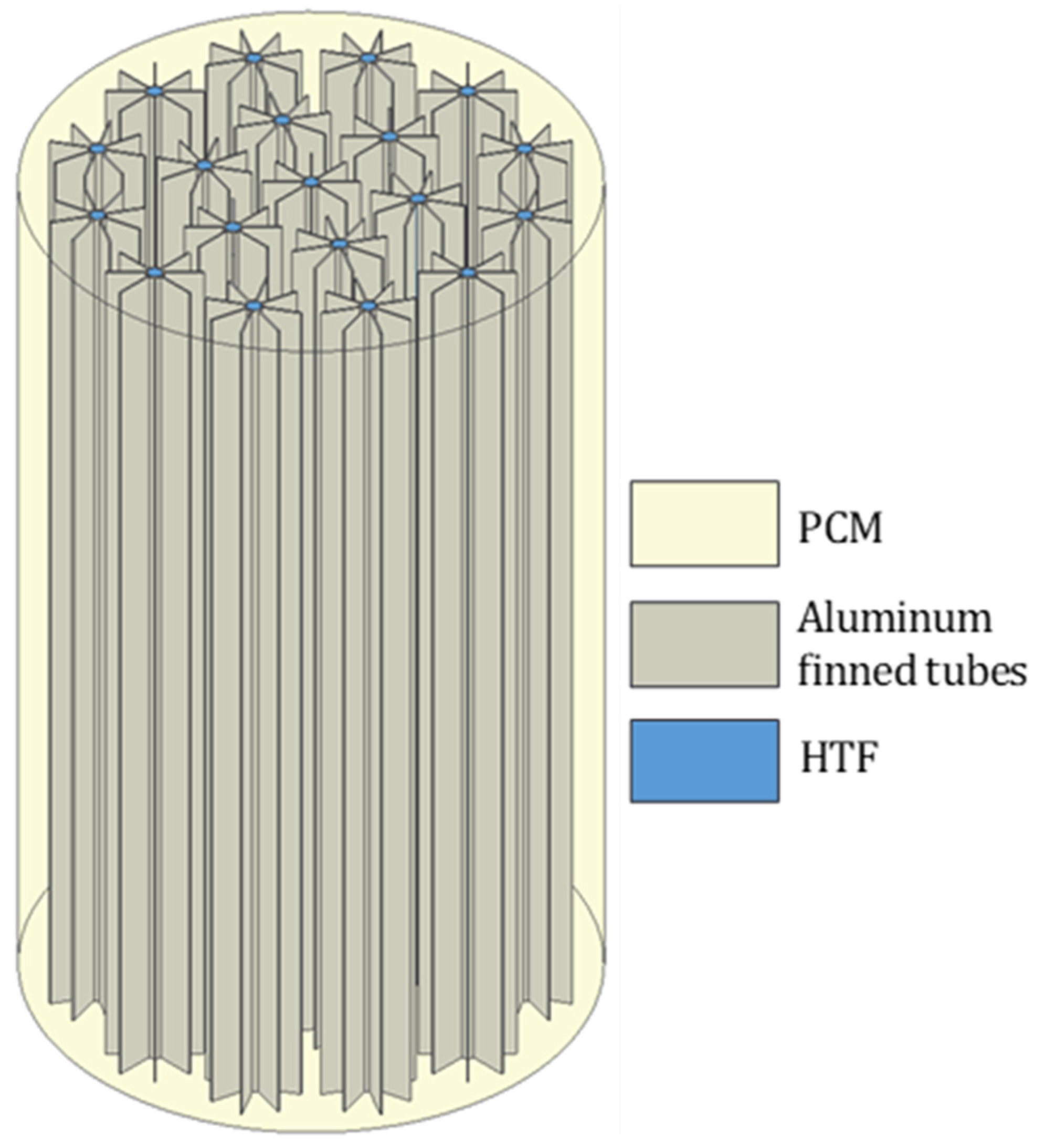
Figure 2.
Top view of the section of analyzed LTES tank.
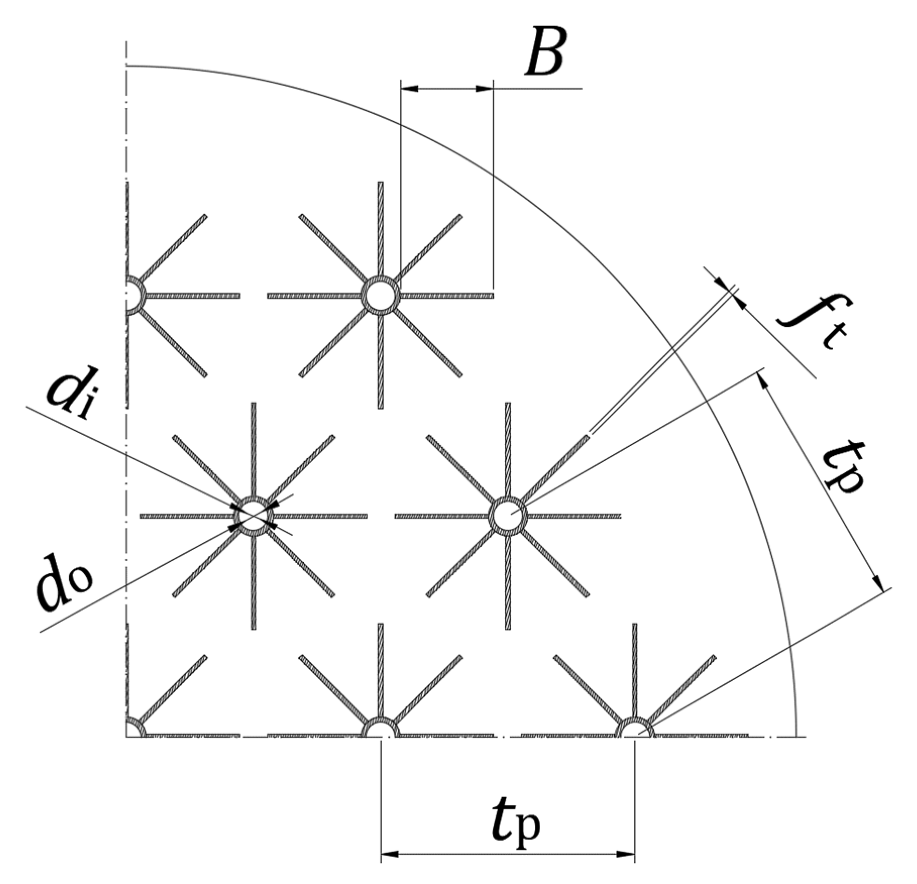
Figure 3.
Schematic representation of a one-dimensional computational model of shell and finned tube LTES and the ith segment.
Figure 3.
Schematic representation of a one-dimensional computational model of shell and finned tube LTES and the ith segment.
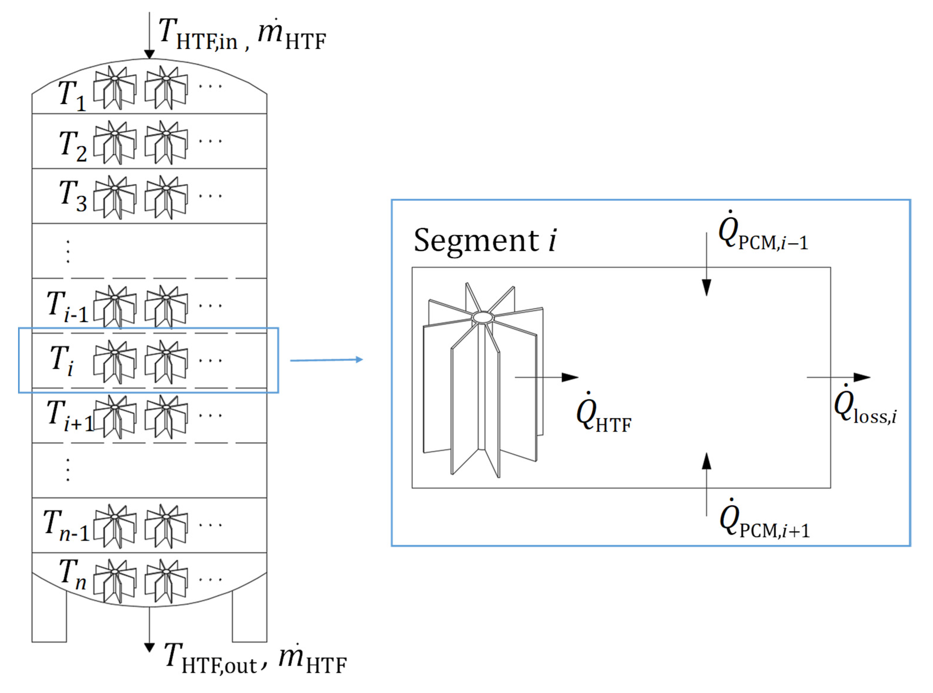
Figure 4.
Schematic representation of a PCM annulus and the detail showing schematic representation of thermal resistances between HTF and PCM.
Figure 4.
Schematic representation of a PCM annulus and the detail showing schematic representation of thermal resistances between HTF and PCM.
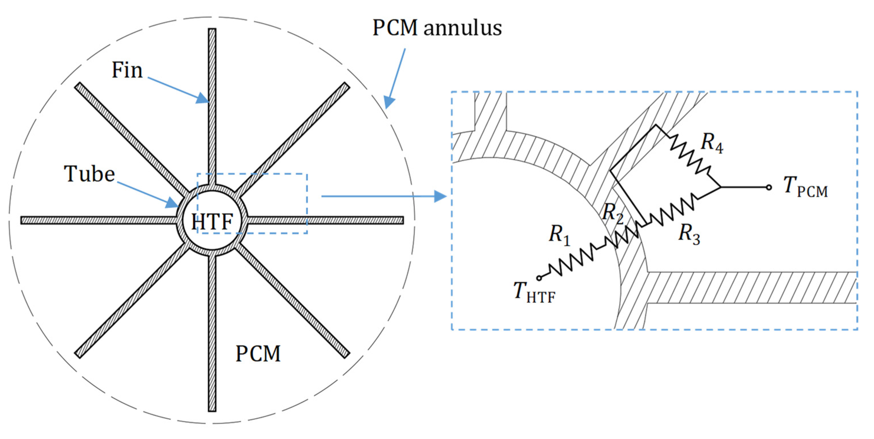
Figure 5.
Transient PCM temperature variations at the middle axial position of LTES during melting for HTF flow rate 620 l/h and HTF inlet temperature 37 °C, obtained by computational model with different number of LTES tank isothermal segments.
Figure 5.
Transient PCM temperature variations at the middle axial position of LTES during melting for HTF flow rate 620 l/h and HTF inlet temperature 37 °C, obtained by computational model with different number of LTES tank isothermal segments.
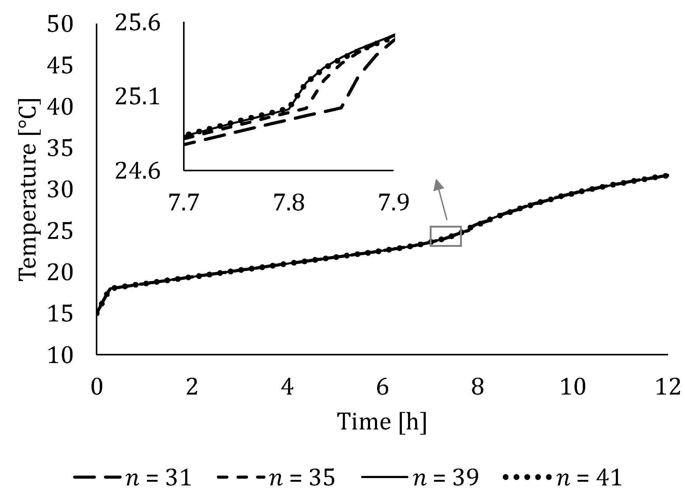
Figure 6.
Transient PCM temperature variations at the middle axial position of LTES during melting for HTF flow rate 620 l/h and HTF inlet temperature 37 °C, obtained by a computational model with different time step sizes.
Figure 6.
Transient PCM temperature variations at the middle axial position of LTES during melting for HTF flow rate 620 l/h and HTF inlet temperature 37 °C, obtained by a computational model with different time step sizes.
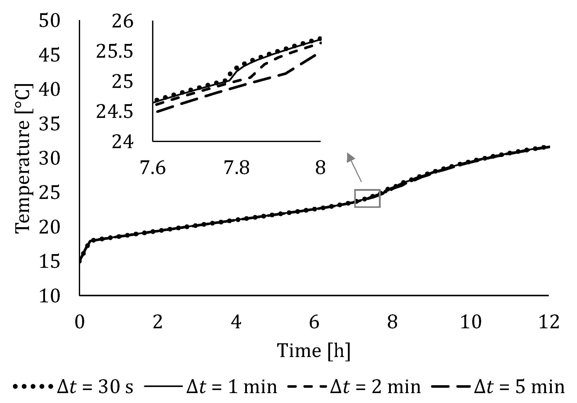
Figure 7.
Schematic representation of an experimental test system segment with LTES tank, HTF flow rate and inlet temperature regulation, cold HTF inlet, cold HTF outlet, hot HTF inlet, and hot HTF outlet.
Figure 7.
Schematic representation of an experimental test system segment with LTES tank, HTF flow rate and inlet temperature regulation, cold HTF inlet, cold HTF outlet, hot HTF inlet, and hot HTF outlet.
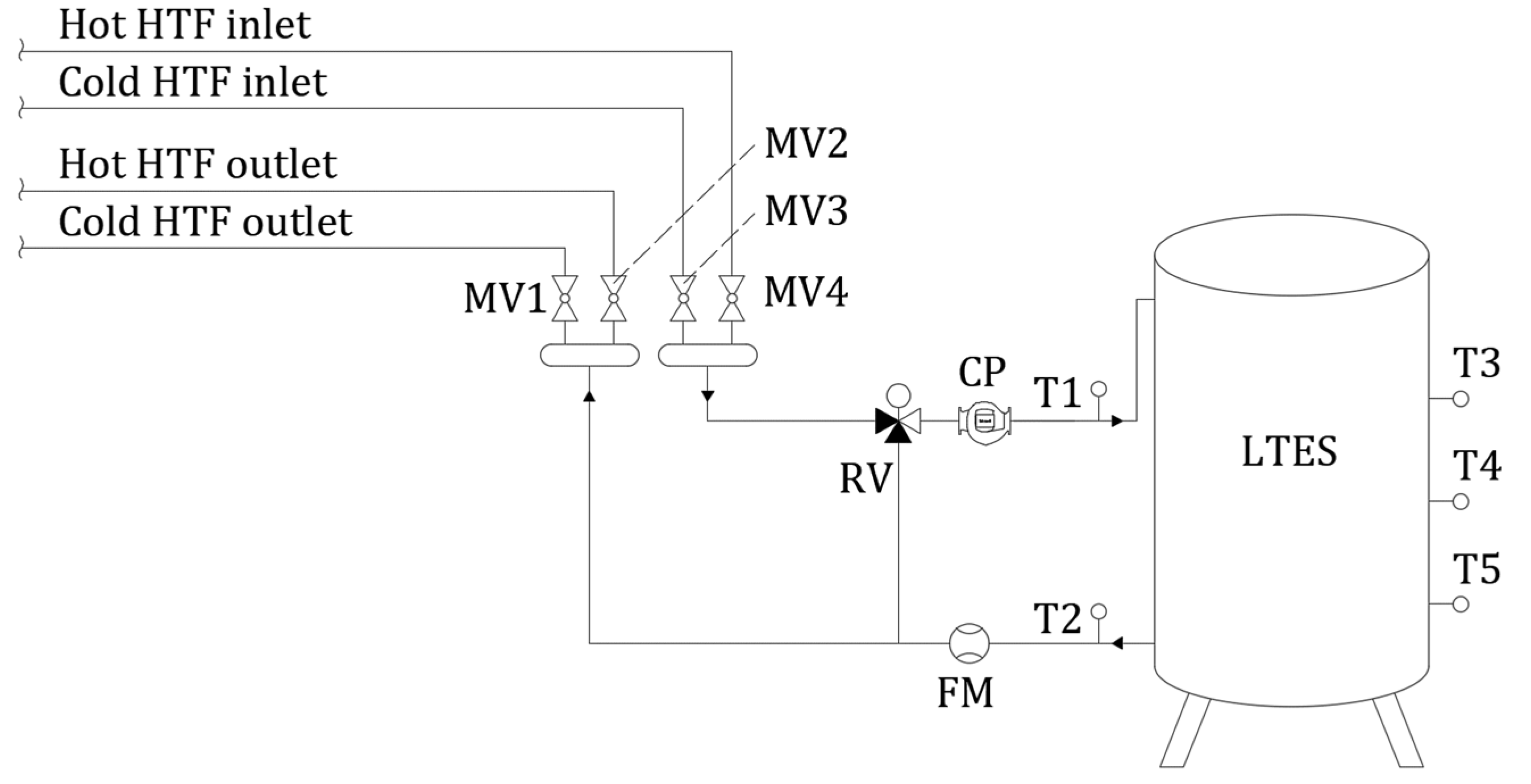
Figure 8.
Experimental LTES tank.
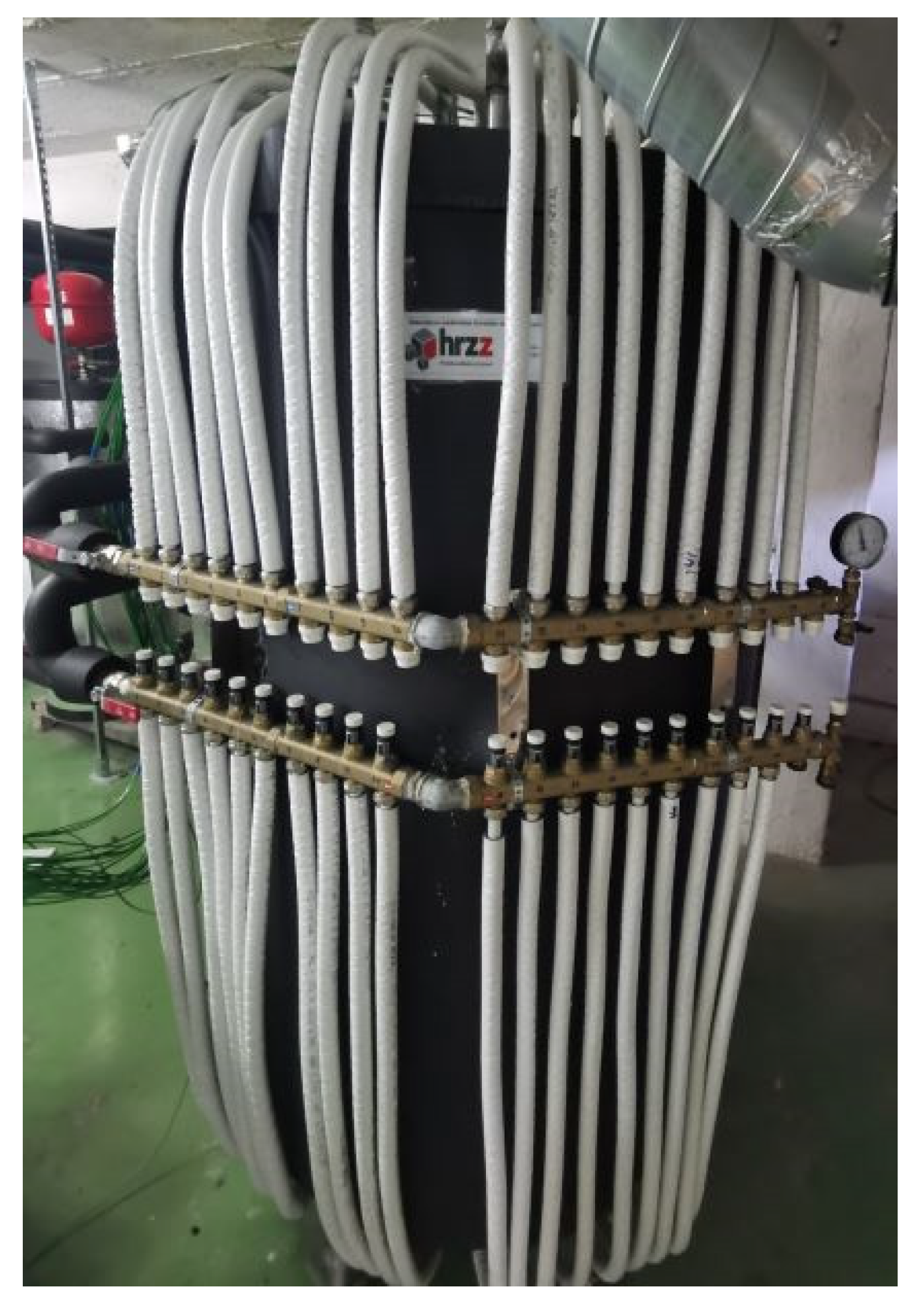
Figure 9.
Comparison of transient temperature variations of the HTF and PCM during melting obtained numerically and experimentally at positions T2, T3, T4 and T5 for HTF flow rate 620 l/h and HTF inlet temperature 42 °C.
Figure 9.
Comparison of transient temperature variations of the HTF and PCM during melting obtained numerically and experimentally at positions T2, T3, T4 and T5 for HTF flow rate 620 l/h and HTF inlet temperature 42 °C.
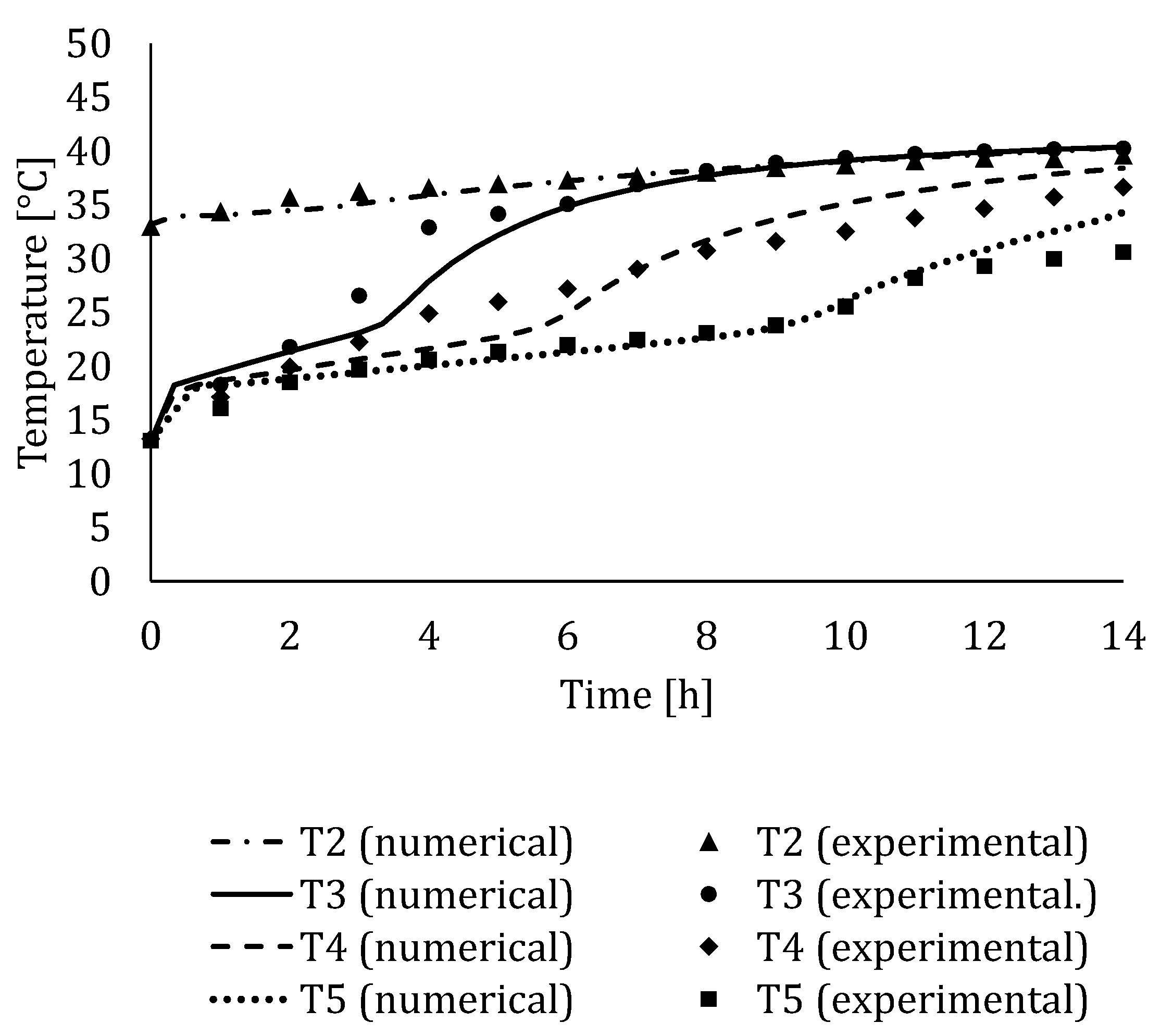
Figure 10.
Comparison of accumulated energy during melting obtained numerically and experimentally for HTF flow rate 620 l/h and HTF inlet temperature 42 °C.
Figure 10.
Comparison of accumulated energy during melting obtained numerically and experimentally for HTF flow rate 620 l/h and HTF inlet temperature 42 °C.
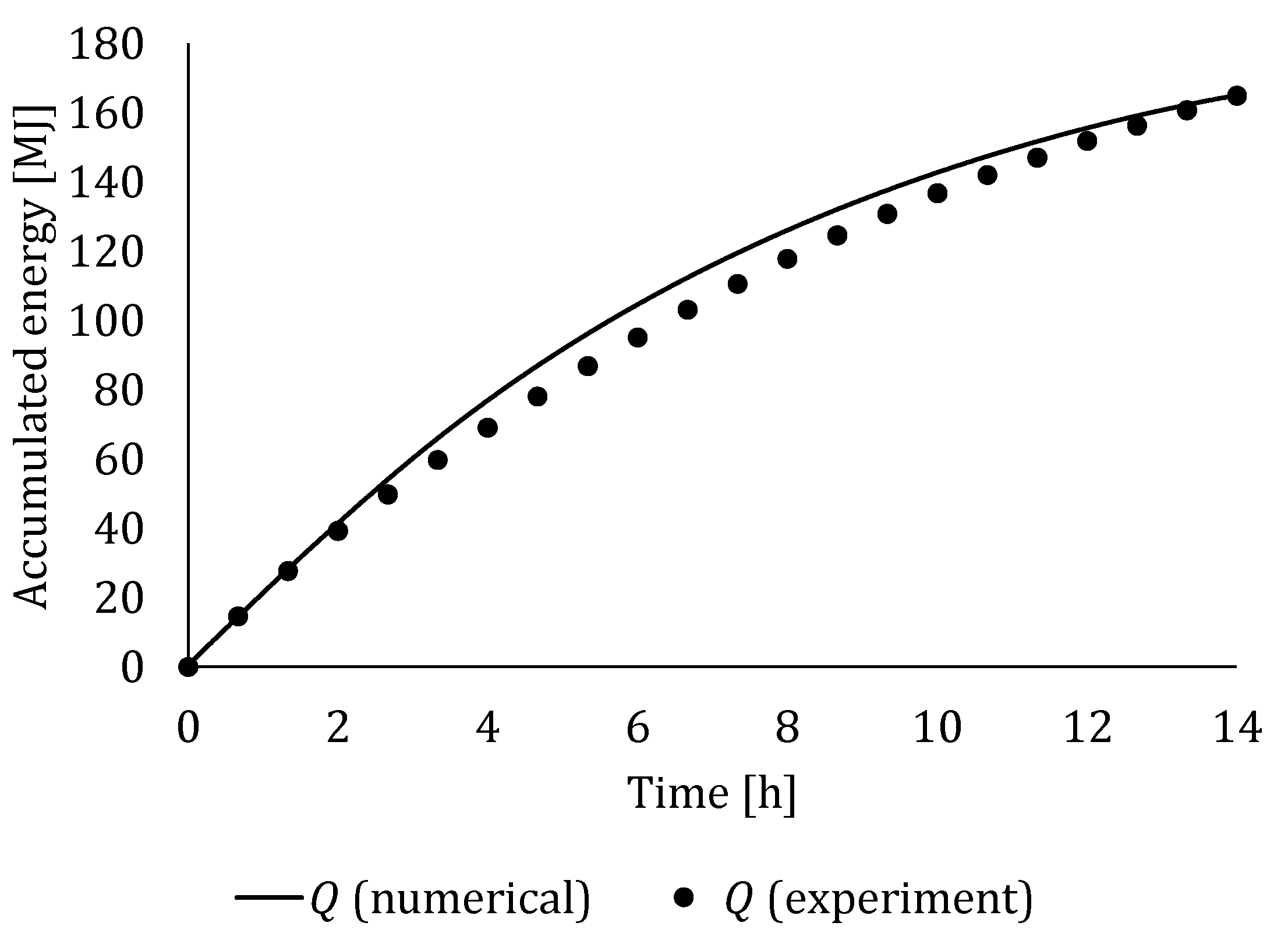
Figure 11.
Comparison of transient temperature variations of the HTF and PCM during solidification obtained numerically and experimentally for HTF flow rate 620 l/h and HTF inlet temperature 7 °C.
Figure 11.
Comparison of transient temperature variations of the HTF and PCM during solidification obtained numerically and experimentally for HTF flow rate 620 l/h and HTF inlet temperature 7 °C.

Figure 12.
Comparison of accumulated energy during solidification obtained numerically and experimentally for HTF flow rate 620 l/h and HTF inlet temperature 7 °C.
Figure 12.
Comparison of accumulated energy during solidification obtained numerically and experimentally for HTF flow rate 620 l/h and HTF inlet temperature 7 °C.

Figure 13.
Comparison of transient variations of PCM temperatures during melting obtained numerically for different HTF inlet temperatures, HTF inlet flow rate 800 l/h and initial PCM temperature 15 °C.
Figure 13.
Comparison of transient variations of PCM temperatures during melting obtained numerically for different HTF inlet temperatures, HTF inlet flow rate 800 l/h and initial PCM temperature 15 °C.
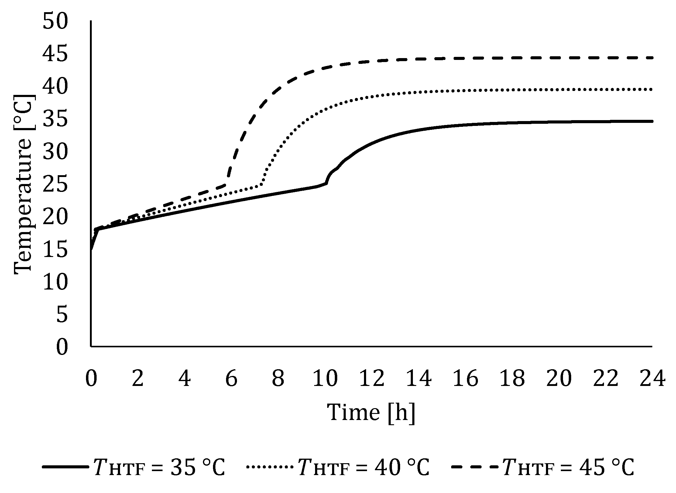
Figure 14.
Comparison of accumulated energy during melting obtained numerically for different HTF inlet temperatures, HTF inlet flow rate 800 l/h and initial PCM temperature 15 °C.
Figure 14.
Comparison of accumulated energy during melting obtained numerically for different HTF inlet temperatures, HTF inlet flow rate 800 l/h and initial PCM temperature 15 °C.

Figure 15.
Comparison of mean heat transfer rates during melting obtained numerically for different HTF temperatures, HTF inlet flow rate 800 l/h and initial PCM temperature 15 °C.
Figure 15.
Comparison of mean heat transfer rates during melting obtained numerically for different HTF temperatures, HTF inlet flow rate 800 l/h and initial PCM temperature 15 °C.

Figure 16.
Comparison of transient variations of PCM temperatures during solidification obtained numerically for different HTF inlet temperatures, HTF inlet flow rate 800 l/h and initial PCM temperature 35 °C.
Figure 16.
Comparison of transient variations of PCM temperatures during solidification obtained numerically for different HTF inlet temperatures, HTF inlet flow rate 800 l/h and initial PCM temperature 35 °C.
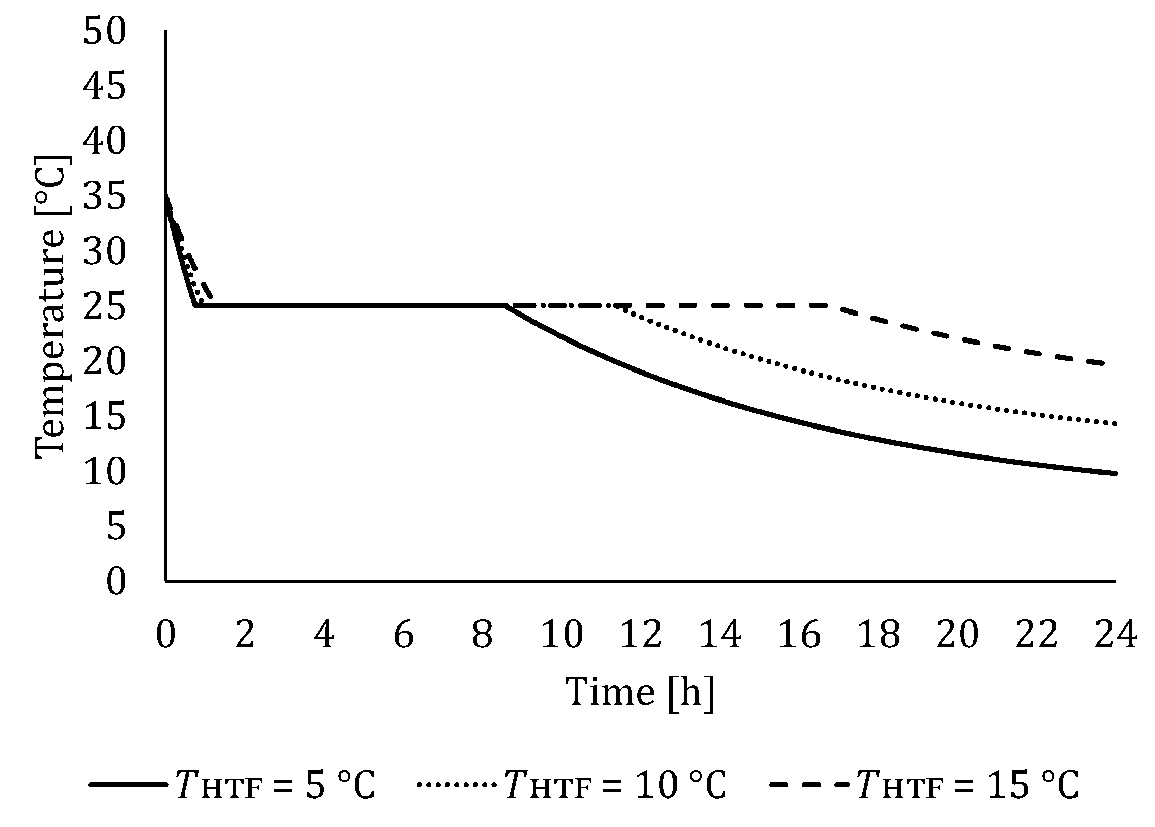
Figure 17.
Comparison of released energy during solidification obtained numerically for different HTF inlet temperatures, HTF inlet flow rate 800 l/h and initial PCM temperature 35 °C.
Figure 17.
Comparison of released energy during solidification obtained numerically for different HTF inlet temperatures, HTF inlet flow rate 800 l/h and initial PCM temperature 35 °C.
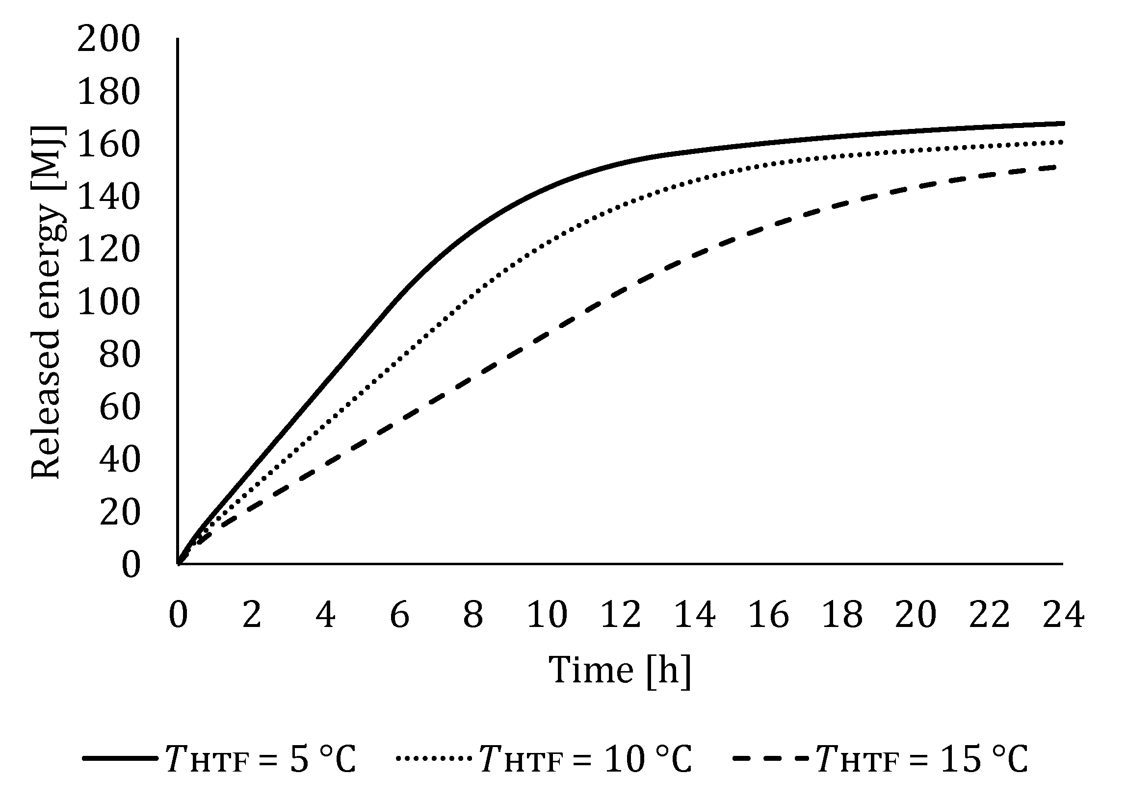
Figure 18.
Comparison of mean heat transfer rates during solidification obtained numerically for different HTF temperatures, HTF inlet flow rate 800 l/h and initial PCM temperature 35 °C.
Figure 18.
Comparison of mean heat transfer rates during solidification obtained numerically for different HTF temperatures, HTF inlet flow rate 800 l/h and initial PCM temperature 35 °C.
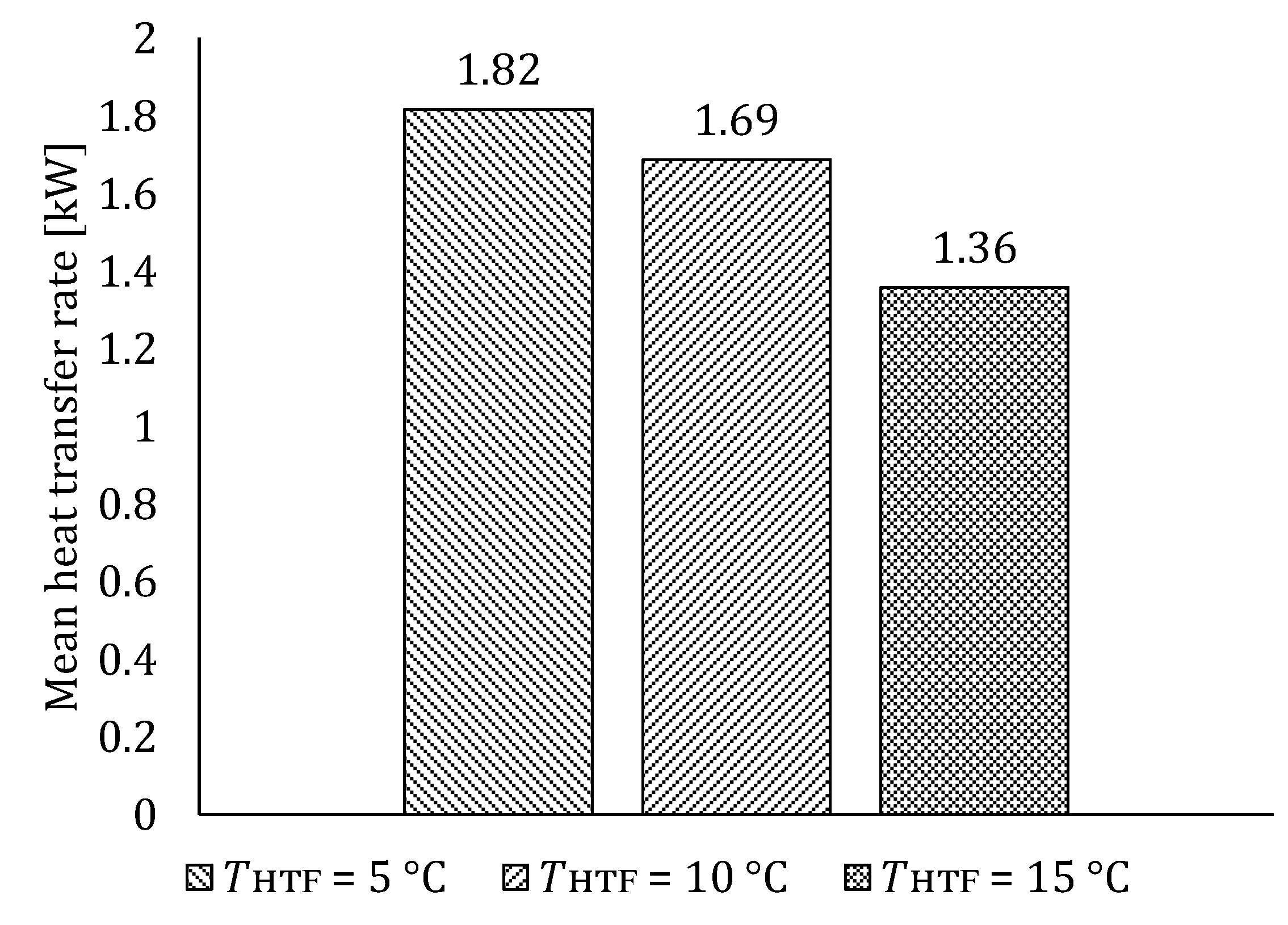
Figure 19.
Comparison of transient variations of PCM temperatures during melting obtained numerically for different HTF flow rates, HTF inlet temperature 40 °C and initial PCM temperature 15 °C.
Figure 19.
Comparison of transient variations of PCM temperatures during melting obtained numerically for different HTF flow rates, HTF inlet temperature 40 °C and initial PCM temperature 15 °C.

Figure 20.
Comparison of accumulated energy during melting obtained numerically for different HTF flow rates, HTF inlet temperature 40 °C and initial PCM temperature 15 °C.
Figure 20.
Comparison of accumulated energy during melting obtained numerically for different HTF flow rates, HTF inlet temperature 40 °C and initial PCM temperature 15 °C.

Figure 21.
Comparison of mean heat transfer rate during melting obtained numerically for different HTF flow rates, HTF inlet temperature 40 °C and initial PCM temperature 15 °C.
Figure 21.
Comparison of mean heat transfer rate during melting obtained numerically for different HTF flow rates, HTF inlet temperature 40 °C and initial PCM temperature 15 °C.
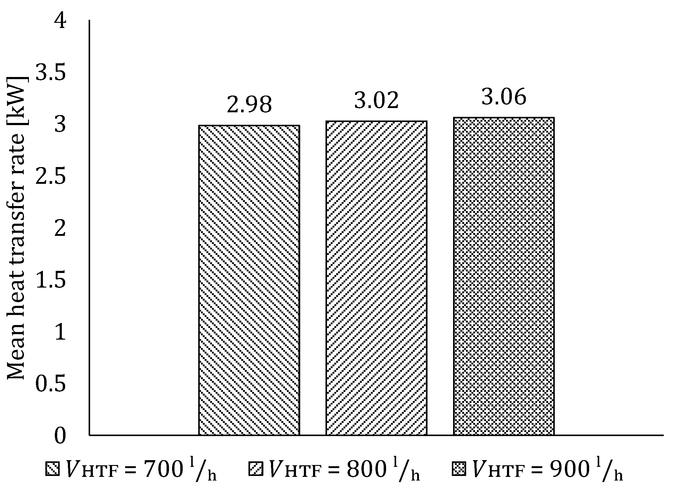
Figure 22.
Comparison of transient variations of PCM temperatures during solidification obtained numerically for different HTF flow rates, HTF inlet temperature 10 °C and initial PCM temperature 35 °C.
Figure 22.
Comparison of transient variations of PCM temperatures during solidification obtained numerically for different HTF flow rates, HTF inlet temperature 10 °C and initial PCM temperature 35 °C.
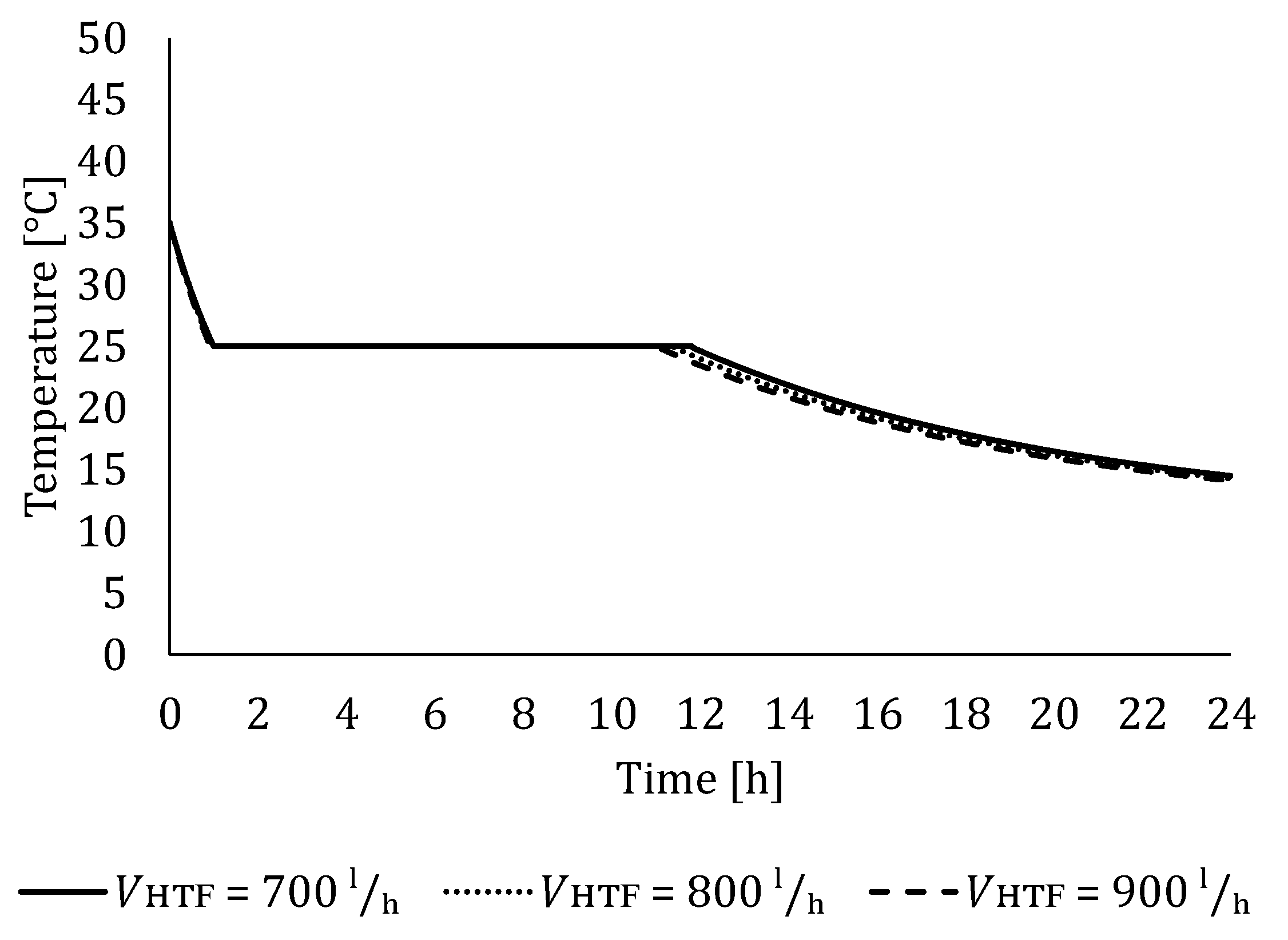
Figure 23.
Comparison of released energy during solidification obtained numerically for different HTF flow rates, HTF inlet temperature 10 °C and initial PCM temperature 35 °C.
Figure 23.
Comparison of released energy during solidification obtained numerically for different HTF flow rates, HTF inlet temperature 10 °C and initial PCM temperature 35 °C.
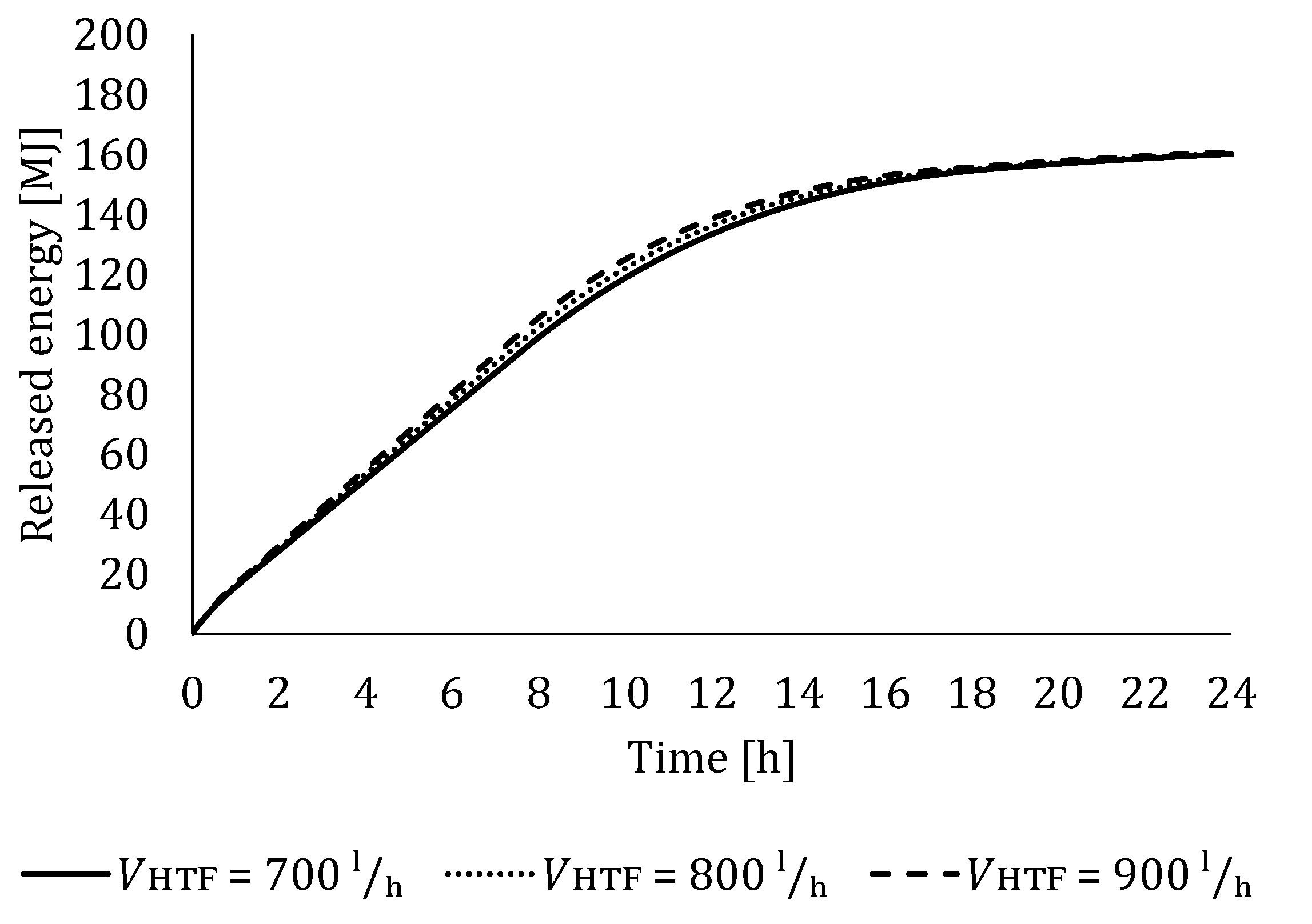
Figure 24.
Comparison of mean heat transfer rate during solidification obtained numerically for different HTF flow rates, HTF inlet temperature 10 °C and initial PCM temperature 35 °C.
Figure 24.
Comparison of mean heat transfer rate during solidification obtained numerically for different HTF flow rates, HTF inlet temperature 10 °C and initial PCM temperature 35 °C.

Table 1.
Geometry parameters of the analyzed LTES.
| LTES tank height, L [mm] | 1550 |
| LTES tank diameter, D [mm] | 950 |
| Tubes diameters, do/di [mm] | 30/25 |
| Number of tubes, nt [-] | 19 |
| Number of fins per tube, nf [-] | 8 |
| Fin thickness, ft [mm] | 1 |
| Fin width, B [mm] | 66 |
| Tube pitch, tp [mm] | 180 |
Table 2.
Thermo-physical properties of PCM paraffin RT25, water and aluminum used in numerical simulations.
Table 2.
Thermo-physical properties of PCM paraffin RT25, water and aluminum used in numerical simulations.
| Properties | PCM | Water | Aluminum | |
|---|---|---|---|---|
| Liquid | Solid | |||
| Density [kg/m3] | 760 | 880 | 998.2 | 2719 |
| Thermal conductivity [W/mK] | 0.2 | 0.6 | 202.4 | |
| Specific heat capacity [J/kgK] | 2000 | 4182 | 871 | |
| Kinematic viscosity of PCM [mm2/s] | 4.7 | 1.005 | - | |
| Latent heat [J/kg] | 170,000 | - | - | |
| Melting | Solidification | - | - | |
| Liquidus temperature [°C] | 25 | 25 | - | - |
| Solidus temperature [°C] | 18 | 25 | - | - |
| Thermal expansion coefficient [1/K] | 0.001 | - | - | |
Publisher’s Note: MDPI stays neutral with regard to jurisdictional claims in published maps and institutional affiliations. |
© 2022 by the authors. Licensee MDPI, Basel, Switzerland. This article is an open access article distributed under the terms and conditions of the Creative Commons Attribution (CC BY) license (https://creativecommons.org/licenses/by/4.0/).
Share and Cite
MDPI and ACS Style
Torbarina, F.; Lenic, K.; Trp, A. Computational Model of Shell and Finned Tube Latent Thermal Energy Storage Developed as a New TRNSYS Type. Energies 2022, 15, 2434. https://doi.org/10.3390/en15072434
AMA Style
Torbarina F, Lenic K, Trp A. Computational Model of Shell and Finned Tube Latent Thermal Energy Storage Developed as a New TRNSYS Type. Energies. 2022; 15(7):2434. https://doi.org/10.3390/en15072434
Chicago/Turabian StyleTorbarina, Fran, Kristian Lenic, and Anica Trp. 2022. "Computational Model of Shell and Finned Tube Latent Thermal Energy Storage Developed as a New TRNSYS Type" Energies 15, no. 7: 2434. https://doi.org/10.3390/en15072434
Note that from the first issue of 2016, this journal uses article numbers instead of page numbers. See further details here.