
Detecting Wind Turbine Blade Icing with a Multiscale Long Short-Term Memory Network

School of Electrical Engineering, Yanshan University, Qinhuangdao 066004, China
*
Authors to whom correspondence should be addressed.
Energies 2022, 15(8), 2864; https://doi.org/10.3390/en15082864
Submission received: 2 March 2022
/
Revised: 28 March 2022
/
Accepted: 12 April 2022
/
Published: 14 April 2022
(This article belongs to the Collection Wind Turbines)
Abstract
:Blade icing is one of the main problems of wind turbines installed in cold climate regions, resulting in increasing power generation loss and maintenance costs. Traditional blade icing detection methods greatly rely on dedicated sensors, such as vibration and acoustic emission sensors, which require additional installation costs and even reduce reliability due to the degradation and failures of these sensors. To deal with this challenge, this paper aims to develop a cost-effective detection system based on the existing operation data collected from the supervisory control and data acquisition (SCADA) systems which are already equipped in large-scale wind turbines. Considering that SCADA data is essentially a multivariate time series with inherent non-stationary and multiscale temporal characteristics, a new wavelet-based multiscale long short-term memory network (WaveletLSTM) approach is proposed for wind turbine blade icing detection. The proposed method incorporates wavelet-based multiscale learning into the traditional LSTM architecture and can simultaneously learn global and local temporal features of multivariate SCADA signals, which improves fault detection ability. A real case study has shown that our proposed WaveletLSTM method achieved better detection performance than the existing methods.
1. Introduction
Wind energy, as a type of clean and renewable energy, has developed rapidly in recent years, and accordingly, the installed capacity of wind turbines has constantly been increasing. Practically, to obtain maximum wind speed, onshore wind farms are usually located in elevated areas such as north China, where blades are often exposed to freezing environments (e.g., low temperatures, high humidity, and air density) and prone to blade icing. As a result, the icing on wind turbine blades will increase high stress on the overall structure and may cause aerodynamic and mass imbalance [1], which results in lowering wind power production and reducing the lifetime [2,3]. If the ice on the blades is not removed in time, it may induce damages to other components coupled with the blades (such as the main bearing) and even secondary major safety accidents. Therefore, it is of great significance for timely detection and elimination of blade icing. Once the blade icing is accurately detected, the de-icing systems can be triggered, thus helping avoid more severe accidents. This paper aims to develop a reliable and accurate blade icing detection system to achieve this goal.
Currently, blade icing detection methods mainly include contact detection methods, hand-held or fixed telescope detection, unmanned aerial vehicle inspection, vibration mode analysis, and infrared scanning. To effectively detect common blade faults, including holes, cracks, and delamination, various methods based on vibration, acoustic emission, and wave propagation are often employed to monitor and assess the health status of wind turbine blades [4,5]. However, these methods are not applicable during the operation of wind turbines and even require additional costs to install cameras or ultrasonic sensors. Moreover, the degradation and failure of sensors may affect the signal accuracy, and reduce the reliability of the ice detection system. Therefore, to address the above drawbacks, it is of great value to develop effective wind turbine blade icing detection systems with timely ice detection, high reliability, and low cost.
Over the last decade, supervisory control and data acquisition (SCADA) based methods have been considered a cost-effective way and have been widely studied [6]. For large-scale wind turbines, the SCADA system has become a standard configuration. It is dedicated to collecting operational data and status data, which contain abundant environmental, electrical, and mechanical parameters related to the health status of wind turbines. Currently, SCADA data have been widely to monitor conditions of major components in wind turbines, including blades [7,8], generators [9,10] and gearboxes [11,12]. For example, Skrimpas et al. [7] utilized the nacelle vibration and power curve data as input to decide for blade icing detection. Dong et al. [13] established a blade icing identification model based on the progressive analysis of different performance parameters change characteristics, including output power, mechanical, aerodynamic performance parameters from SCADA data. Rezamand et al. [14] developed a hybrid wind turbine blade fault detection system based on recursive principal component analysis (PCA) and wavelet-based probability density function (PDF) and successfully detected incipient blade failures. However, monitoring blade with SCADA data is a great challenging task due to the following reasons:
- SCADA data usually do not contain measurements related to a wind turbine blade health status, such as blade vibrations and mechanical loads;
- Available SCADA variables cannot directly reflect the health condition of wind turbine blades;
- Most existing methods greatly rely on manual feature extraction and shallow machine learning methods and cannot achieve satisfactory performance due to their limited modeling ability with the shallow network architecture.
To address the above challenges, this paper aims to develop a cost-effective wind turbine blade icing detection system with SCADA data and investigate deep learning models to perform effective SCADA data modeling and analysis. Deep learning has been considered a powerful feature learning and modeling tool. It has achieved excellent performance in various challenging tasks, especially in computer vision and natural language processing. Its core idea is to learn important and representative representations from input data adaptively through a deep neural network with multilayer nonlinear transformations. Inspired by the superior performance of deep learning, deep neural networks (DNNs) have been considerably applied for wind turbine health monitoring and fault diagnosis [15,16,17,18]. Wang et al. [19] designed a deep autoencoder model and derived the reconstruction error-based health index to identify the possibility of wind turbine blade breakage. Later, in [20], a conditional convolutional autoencoder-based method was proposed to detect wind turbine blade breakages and achieved better performance than classical autoencoder-based methods.
However, SCADA data naturally are multivariate time series, which are characterized by strong temporal dependence for each sensory variable, which is often changing over time and will be impacted by the change of the external environments [21]. On the other hand, since wind turbines are driven stochastically by the external wind, SCADA data usually present non-stationary characteristics and are subject to various disturbances and noises. Considering the multivariable, multiscale, dynamic time-varying, known-stationary characteristics of SCADA data, those existing methods cannot deal with these issues well. Most methods only consider the global characteristics of each sensor variable in SCADA, while local characteristics of different variables are often ignored. In a pioneer study, Yuan et al. [22] proposed a wavelet-based fully convolutional neural network (WaveletFCNN) model to detect blade icing faults. However, the WaveletFCNN does not consider the inherent but important temporal dependence of SCADA data. Inspired by the above pioneer work and aiming to overcome the limitation of the existing WaveletFCNN model, this paper proposes a new wavelet-based multiscale long short-term memory network named WaveletLSTM to learn the global and local features of multivariate SCADA data simultaneously and then accurately detect blade icing conditions of wind turbines.
The specific contributions of this paper are two-fold. Firstly, a new WaveletLSTM model is proposed based on the traditional LSTM but incorporates the ability of multiscale learning by introducing wavelet transform. It can learn complementary diagnostic information from global and local scales in parallel and obtain enhanced multiscale feature representations with more discriminability. The proposed WaveletLSTM can enhance feature extraction ability against the traditional LSTM that handles only a single timescale. Secondly, we develop a novel WaveletLSTM-based blade icing detection system for wind turbines, which can automatically learn informative features from raw multivariate SCADA data and its wavelet-based decomposed local signals and then identify blade icing conditions. Our proposed model is evaluated using real SCADA data from a wind farm, and the results show that our WaveletLSTM model achieved better fault detection performance compared with several deep learning-based methods and three shallow machine learning methods in terms of five classification metrics. Additionally, this design requires no expert knowledge and has the potential to provide a general-purpose fault detection solution for industrial applications.
The rest of this paper is organized as follows. Section 2 briefly reviews LSTM and its applications for fault detection and diagnosis. Section 3 details the proposed WaveletLSTM model for wind turbine blade icing fault detection. Section 4 presents a case study to evaluate the performance of our proposed method. Lastly, conclusions are drawn in Section 5.
2. A Brief Overview of LSTM and Its Application in Fault Detection and Diagnosis
Our proposed WaveletLSTM model is developed based on a standard LSTM network. In this section, we first give a brief overview of the basic principle of LSTM and then review the related works about LSTM for fault detection and diagnosis.
2.1. Overview of Long-Short Term Memory Network
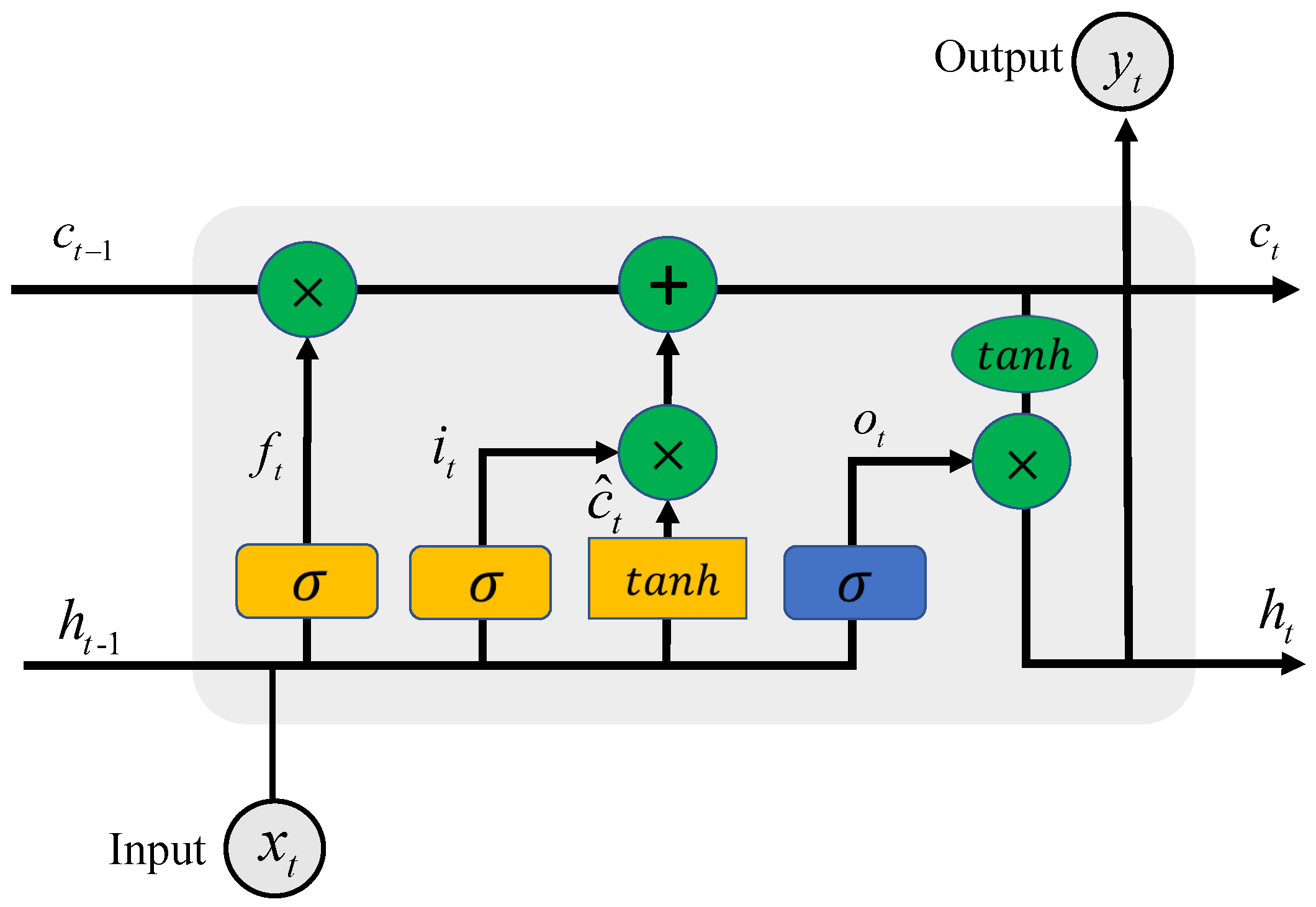
The LSTM network is a variant of the traditional recurrent neural network (RNN), which was first proposed in 1997 by Hochreiter and Schmidhuber [23]. LSTM was developed to deal with the exploding and vanishing gradient problems encountered when training traditional RNNs. LSTM is explicitly designed to learn the long-term dependencies for modeling sequential data (e.g., time series). A typical feature of LSTMs is the introduction of the gate mechanism. Specifically, an LSTM cell introduces three gates: input gate , forget gate and output gate . The input gate can select key information stored in the internal state. The forget gate will discard some redundant information. Finally, the output information can be identified by the output gate. These gates are used to control the pass of new knowledge, which are updated as follows:
where is the sigmoid activation function, all W and b are model parameters to learn, and the operator ⊙ presents the element-wise multiplication. Figure 1 shows a brief schematic diagram at time step t of an LSTM unit structure.
2.2. LSTM for Fault Detection and Diagnosis
Recent studies have shown that LSTM has an excellent performance in sequence learning and modeling with various applications, such as image caption, speech recognition, natural language processing and time series forecasting [24,25,26]. Motivated by the successful achievements of LSTMs in time-dependent prediction and classification tasks, LSTM has been recently applied to the field of fault detection and diagnosis to deal with different temporal sensor signals from various monitored machines, such as aero-engines, gas turbines and wind turbines. For example, Yang et al. [27] proposed an LSTM-based fault detection and isolation approach for electro-mechanical actuators in the aircraft system, in which an improved LSTM was developed to learn correlations between sensors and obtain better detection performance. In [28], Bruin et al. used LSTM recurrent neural network to process the signals from multiple track circuits in a geographic area and learn the spatial and temporal dependencies directly from data. The results demonstrated that the LSTM network achieved a fault diagnosis accuracy of 99.7% with no false-positive fault detections.
In terms of wind turbine fault detection applications, several related works have been recently reported. Xue et al. [29] developed an LSTM-based fault detection method to detect different fault types of an open-circuit switch of the back-to-back converter in wind turbine systems. Lei et al. [30] developed an end-to-end LSTM model to learn features from multivariate time-series data and realized the multi-class fault diagnosis of wind turbine bearings. In [31], Li et al. proposed an LSTM-based data-driven fault diagnosis and isolation method, where an LSTM-based residual generator was first constructed. Then the random forest algorithm was applied for decision making. The above works have shown the feasibility and effectiveness of LSTM for wind turbine fault detection and diagnosis. Inspired by these achievements, we focus on investigating multiscale characteristics of SCADA data, which the traditional LSTM ignores.
3. WaveletLSTM for Wind Turbine Blade Icing Detection
3.1. Overall Framework
We formulate blade icing detection as a binary classification issue in this study. Figure 2 shows the overall architecture of the proposed WaveletLSTM model. The model input is raw multivariate time-series data from multiple sensors installed in wind turbines. The model output is a binary classification result, normal or blade icing. The WaveletLSTM is an end-to-end learning architecture that consists of three sequential parts: multiscale decomposition, temporal feature learning, and classification.
- The multiscale decomposition stage applies discrete wavelet decomposition on each input SCADA variable to obtain different local signals;
- In the temporal feature learning stage, we use several staked LSTM layers to extract features for each decomposed level at a local scale and raw data on a global scale. In this stage, the temporal feature learning at different scales is independently from each other;
- In the classification stage, the extracted features from all scales are concatenated and go through a fully connected layer and a softmax layer for final binary classification.
The proposed WaveletLSTM architecture effectively combines the temporal feature learning from the global scale and multiple local scales. It, therefore, enhances the classification performance, as will be shown in the experimental results in Section 4.
3.2. WaveletLSTM Architecture
The input of the WaveletLSTM is the multivariate SCADA time series with size , where N is the length of each sensory time series and D is the number of sensor variables.
3.2.1. Wavelet-Based Multiscale Decomposition
To capture the multiscale characteristics of the SCADA time series, discrete wavelet decomposition is adopted. Each sensor variable time series can be decomposed into a set of wavelet coefficients. The decomposed wavelet coefficients represent the variance of the sequence across different frequency resolutions [32]. As shown in Figure 2, the original time series signal is first decomposed into a detailed coefficient and an approximate coefficient at Level 1. Then the obtained approximate coefficient will be further decomposed at Level 2. Such a decomposition process will be repeated until the target decomposition level of the wavelet is reached. As a result, the original multivariate SCADA time series will be finally decomposed into several wavelet coefficients at different levels, and the size of the wavelet coefficient at ith decomposed level is , where .
Note that the original signal and all decomposed detailed coefficients at different levels are input to the individual deep LSTM model for temporal feature learning in the next stage. Our proposed WaveletLSTM does not consider the obtained approximation coefficient as input since it represents some smooth average of the input signal, which can be easily learned when processing the original signal. Additionally, this will reduce the redundancy of the input and the difficulty of model training.
3.2.2. LSTM-Based Temporal Feature Learning
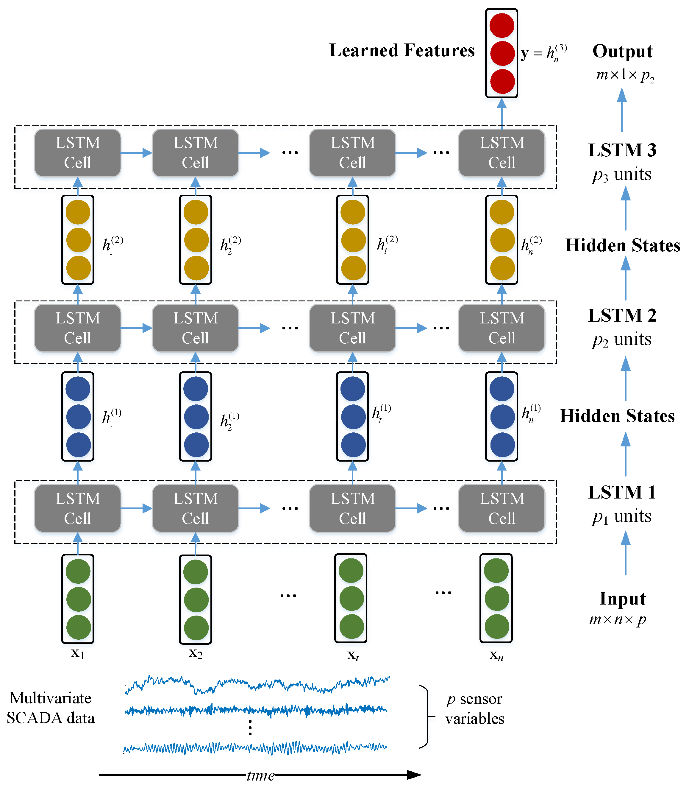
Herein, a deep LSTM model with multiple LSTM layers is designed to learn temporal features hidden in multivariate times series. Figure 3 shows an illustration of a three-layer deep LSTM architecture for temporal feature learning. The model input is a multivariate time series with a size of , where and p represent the number of time series samples, the temporal length of each sample and the number of sensor variables, respectively.
For the original signal and all decomposed wavelet coefficients, temporal feature learning is performed separately, as shown in Figure 2. It should be noted that global and local temporal features can be learned from the original signal and all decomposed wavelet coefficients, respectively, and thus can provide much more information for the subsequent classification task. Specifically, with a given sequential input at time t, its feature representations can be obtained with a deep LSTM model as follows:
where represents the learned model parameters of the DeepLSTM model.
We consider the final hidden state the learned feature representations, which encode the most information from input signals.
3.2.3. Feature Fusion and Classification
In this stage, the learned temporal features from the global view and local view are fused by a simple concatenation way, as shown in Figure 2, which is formulated as a long feature vector. Then, the concatenated feature vector is directly input to a softmax layer to identify whether it is normal or blade icing.
Similar to the traditional LSTM, we train the WaveletLSTM using stochastic gradient descent (SGD) through the back propagation (BP) algorithm. A dropout layer follows each LSTM layer in the temporal feature learning stage to reduce the overfitting risk.
3.3. Online Fault Detection
Once the WaveletLSTM model is well trained, it can be used for online fault detection. For unseen test data, it should be noted that if they are directly input to the trained WaveletLSTM model to output classification results, there will be a large probability of misclassification risks. Therefore, to generate a more accurate and robust detection result, we adopt a recently proposed anomaly detection algorithm based on a sliding window and majority voting [22]. Since the final decision result is based on the majority vote principle, this model will effectively reduce misclassifications and produce more reliable detection results.
Figure 4 shows the online detection illustration based on the sliding window and the majority vote. For the multivariate time series collected from the SCADA system, it will be first divided into several segments by using a sliding window with the size of and sliding step size . Assuming that the time series is segmented into blocks of length , the sliding window of length will move along the input time series by a step size of . The trained classifier will then predict the time series within the sliding window. Each time the sliding window moves, a prediction will be produced. For example, the WaveletLSTM classifier produces a predicted value when the sliding window slides once and a second predicted value when it slides a second time. Similarly, when sliding the i-th time, the time series module will generate the predicted value . Thus, as the sliding window moves along the signal, each block will accumulate predicted values. To make the final prediction result, the majority voting is adopted to determine whether the current block is abnormal or not, depending on a proper threshold . If the proportion of positive prediction is greater than or equal to the threshold , it will generate an overall positive prediction, which means an anomaly is detected and then will trigger a warning; otherwise, a negative prediction will be generated, which means the system is normal.
4. Case Study
4.1. SCADA Data Description
The available SCADA data used in this study are provided by GoldWind Inc, collected from three wind turbines in a wind farm located in north China. The data sampling interval is 7 s, and the time range is from 1 November 2015 to 1 January 2016. During this time period, the weather is fairly cold (e.g., the environmental temperature will be below 0). Accordingly, wind turbine blades are easy to freeze in a large area. Originally, the wind turbine SCADA data contained hundreds of dimensions, with a large amount of redundant and unrelated information with blade icing. Therefore, 26 continuous variables related to blade icing are screened by wind turbine manufacturers according to domain-specific knowledge, and a detailed description is given in Table 1. These 26 variables could be grouped into the following four classes:
- Wind parameters, such as wind speed and wind direction measured, which are direct drivers of wind turbines closely affecting the operating conditions, and related to other parameters (e.g., power and pitch angle) [33];
- Temperature parameters including the temperatures measured at turbine components (e.g., pitch motor, pitch battery cabinets), nacelle temperature and external environmental temperature. Blade icing will cause aerodynamic and mass imbalance and induce the temperature changes of pitch motors and pitch battery cabinets [8,13];
- Vibration parameters involving nacelle acceleration in both X and Y directions. Related works have shown that blade ice accretion will result in excessive nacelle oscillation [7].
Previous studies have shown that different variables in SCADA data are highly correlated [34]. The occurrence of a fault or malfunction in a certain component or subsystem may cause changes in multiple variables. Here, correlations between the above variables are investigated. Figure 5 shows the pair plot of several representative variables listed in Table 1, including wind speed, power, pitch angle, acceleration, etc. Note that all data are not original data and have been normalized with the arbitrary unit, which is performed by the data provider (GoldWind Inc., Beijing, China) due to the data confidentiality. It can be seen from the power curve shown in the first subplot that the blade icing causes the reduction of the output power and the change in the aerodynamic performance of wind turbines. Pitch angle vs. wind speed curve shows that most blade icing happened in the rated wind speeds. Acceleration and temperature curves also demonstrate certain differences between icing and normal conditions. In fact, blade icing may lead to the changes of such complex correlations hidden in multivariate data, which has also been studied in [8,22]. Therefore, we aim to extract informative features beneficial for detection from multivariate temporal correlated data.
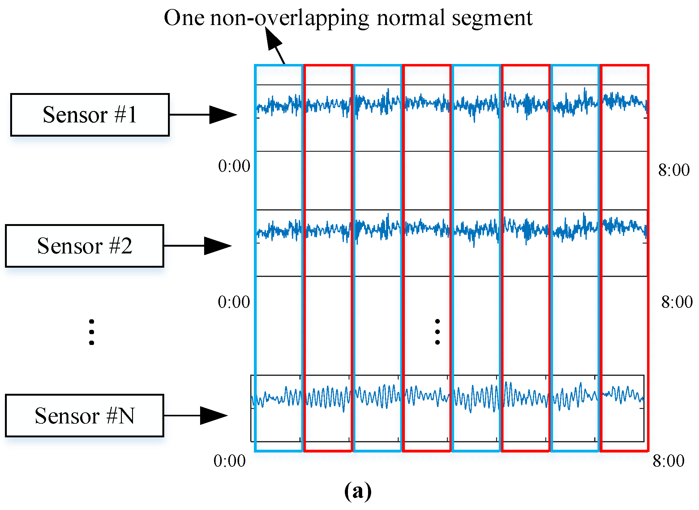
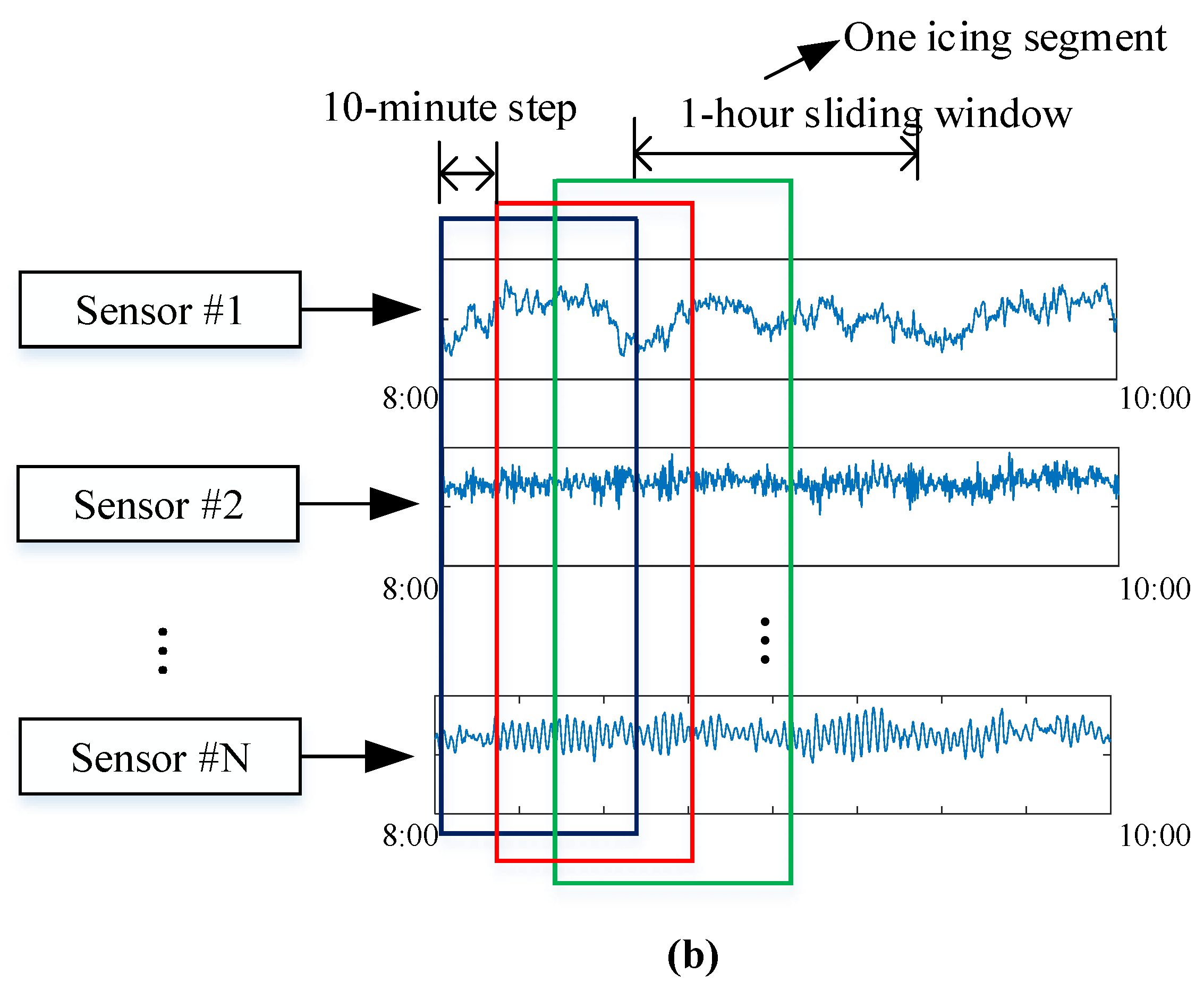
For data labeling, the engineers from wind turbine manufacturing have provided initial normal and icing labels for data samples based on the fault or maintenance log. For simplicity, we denote the icing samples as Label 1, and normal samples as Label 0, respectively. Regarding the data processing, we used the same procedures in [22] to generate the dataset for model training and evaluation. Figure 6 shows the variations of data labels of one turbine in the time domain from 1 November 2015 to 1 January 2016. We can observe that the blade icing accretion happens intermittently. The data portions of normal and blade icing states are quite different. In other words, there exist obvious data imbalance problems between normal and icing conditions, which will produce biased performance if directly using such an imbalanced dataset for detection model training and evaluation. To address this issue and to effectively train our proposed WaveletLSTM model, we introduce a data augmentation strategy with a sliding window technique, which has been used in [22], to generate a balanced dataset for model training and evaluation. Specifically, for normal sample generation, we cut the original normal ranges into several normal segments without overlap, while for icing conditions, the number of icing samples is augmented by generating overlapping icing segments with a fixed-length sliding window with overlap. To be concrete, we give an illustrative diagram of the data sample generation procedure for normal samples and icing samples, as shown in Figure 7. In Figure 7a, we assume that a wind turbine is working at 0:00–8:00, then the normal range without overlap is cut into 8 normal segments, each corresponding to the state within one hour. In Figure 7b, when the blade icing fault occurs in the wind turbine at 8:00–10:00, we can use a 10-min step and a 1-h sliding window to move along the blade icing range, and 7 icing segments (e.g., 8:00–9:00, 8:10–9:10, etc.) are generated. The step size used in our study is 16 (representing a step size of 112 s) to create a balanced dataset. The original signal is divided into a group of fixed-length segments (the length of the fixed-length segment used in this paper is 512), and each segment has a binary label (that is, 0 or 1,1 represents icing, and 0 represents normal) to indicate whether the blade freezes during this period. According to the above principle, an augmented dataset will be finally generated. We further split the augmented dataset into the training set, the validation set and the test set, as summarized in Table 2. The performance of our proposed WaveletLSTM model is further evaluated on such three generated datasets. The training set is used for model training, the validation set is used for model hyperparameter optimization, and the test set is used for model performance evaluation.
4.2. Parameter Setup
For all model training, we used Adam for network optimization for its efficient computation and little memory. Model hyperparameters are experimentally determined based on the validation dataset. To improve the training speed, the training set is split into small batches to update the network weights, and the mini-batch size is set as 12. The learning rates and the number of epochs in the training process are set to 0.01 and 100, respectively. To uniformly convert data of different magnitudes into the same magnitude, the Z-score standardization is used to standardize the data. The settings for LSTM layers are as follows: three hidden layers, each with hidden neuron sizes of 128, 64, and 32, respectively. To prevent the over-fitting of the model in the training process, the dropout layer is added after each LSTM layer to achieve the regularization effect to a certain extent. In this study, the dropout rate is set to 0.3. We use cross-entropy as the loss function which has been widely used in literature [22,26]. The wavelet decomposition level is set to 4, and the mother wavelet function uses haar. Two important parameters, wavelet decomposition scale and model depth, will be discussed in detail in Section 4.5.
In the online detection phase, the sliding window is set to be the same length as the segment in the training set. In this study, The sliding step size is set to , where L is the wavelet decomposition level used in the first step of WaveletLSTM model.
4.3. Evaluation Metric
The blade detection problem studied in this paper can be regarded as a binary classification. To comprehensively evaluate the model performance, the Receiver Operating Characteristic (ROC) curve and the resulting Area Under Curve (AUC) [9,35], the detection accuracy, precision, recall, and F1-score are used as evaluation metrics, which are generally calculated based on the classification results of positive (icing) and negative (normal) samples, which can be represented as a confusion matrix including four parts, i.e., true positive (TP), false positive (FP), true negative (TN) and false-negative (FN). The corresponding calculation formulas are denoted as follows:
4.4. Performance Evaluation and Comparison
To demonstrate the detection performance of our proposed WaveletLSTM model, the traditional LSTM is first compared, which actually can only learn global features from the original multivariate SCADA time series. We also considered another model named WaveletLSTM_ng that only considers the learning ability of local temporal features from the decomposed wavelet coefficients. Differently from LSTM and WaveletLSTM_ng, WaveletLSTM can simultaneously learn global and local features from multiple scales. The compared results of three models are shown in Figure 8, where the numbers represent the AUC values of each model. For WaletLSTM_ng and WaveletLSTM, the number of wavelet decomposition levels is set to 4, and other parameters are consistent. As can be seen from Figure 8, our proposed WaveletLSTM model is expected to achieve the best performance with the AUC value of 0.96. This proves the importance of concurrent learning of global and local features in the fault detection task. Additionally, we notice that the WaveletLSTM_ng model performs worse than LSTM, which means that the global feature learning is more effective than local feature learning. A possible reason for this is that the original data may contain more useful information beneficial for fault detection. At the same time, decomposed detailed wavelet coefficients lose some important information, resulting in poor performance.
Furthermore, we compared our proposed WaveletLSTM model with the existing two models, namely fully convoluted neural networks (FCNN) and wavelet fully convolutional neural networks (WaveletFCNN, both of which are used for wind turbine blade icing detection in [22]. To make a fair comparison, for WaveletFCNN and WaveletLSTM, the wavelet decomposition level was set to the same value of 4. For FCNN and WaveltFCNN, the convolution layer was set to 3, the number of convolution kernels in each layer was 128, 256, 128, and the size of convolution kernels was 8, 5, and 3, respectively. The step size was set to 1, and the activation function of each convolution layer was Relu. The remaining parameters are the same as the settings in [22], and a more detailed description of WaveletFCNN can be found in [22].
As can be seen from Figure 8 our proposed WaveletLSTM classifier performs better than the WaveletFCNN and FCNN in terms of AUC metric. Additionally, WaveletLSTM achieves an FDR of over 0.9 at a lower FAR of 0.1, and the performance is the best among all considered methods. This further shows that it is very important to deeply mine the temporal information of SCADA data to improve fault detection capability. In short, the results prove that our proposed WaveletLSTM model can effectively detect blade icing conditions.
To check more details of classification results, we calculated the confusion matrices of different methods, and the results are shown in Figure 9. Additionally, the derived classification performance metrics are calculated as listed in Table 3 where the best values are highlighted in bold. From Figure 9, it can be seen that our WaveletLSTM successfully predicted 106 of a total of 107 icing cases meaning a higher fault detection rate (FDR) and correctly predicted 1799 of a total of 1795 normal cases. A total of 176 normal cases were wrongly classified as icing ones, which led to false alarms. In terms of FDR, WaveletLSTM and FCNN perform significantly better than WaveletFCNN and LSTM. In terms of FAR, WaveletLSTM achieved the lowest FAR among the four considered models, which produced more reliable fault detection results in practical applications. Classification metrics listed in Table 3 also prove that our proposed WaveletLSTM model exhibited the best performance.
4.5. Parameter Analysis
The proposed WaveletLSTM model involves two important parameters: scales (i.e., wavelet decomposition level) and depths (i.e., the number of hidden layers). Their effects on the model classification performance are investigated as follows.
4.5.1. Effects of Scale
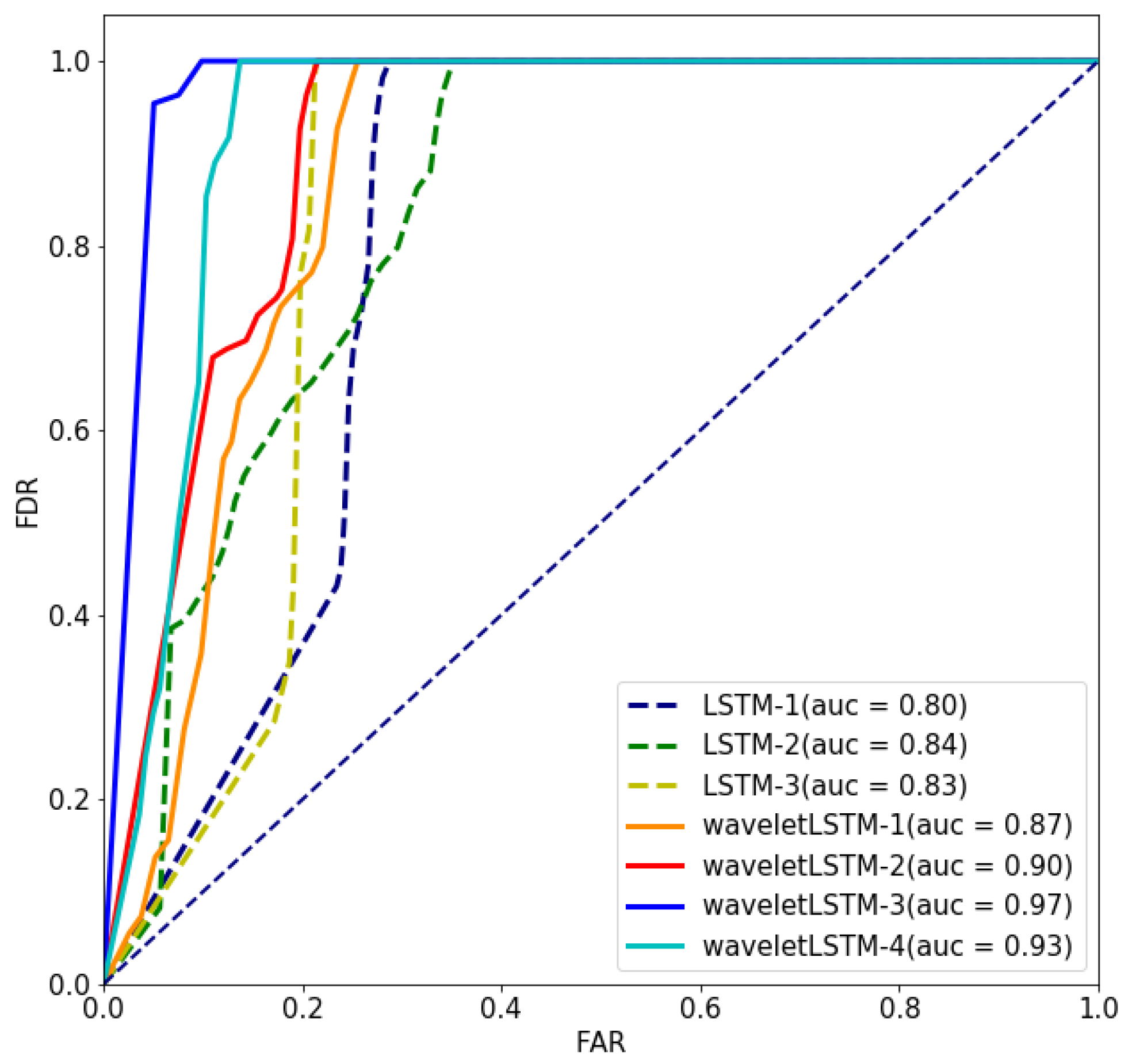
Since SCADA data usually show large variations at different observation scales, it is necessary to consider multi-scale information. In this study, to explore the effects of the scale of WaveletLSTM model on the detection performance, different scales are considered. Traditional LSTM, corresponding to WaveletLSTM with one scale, is also compared. Figure 10 shows the detection performance of WaveletLSTM with different scales in terms of the ROC curves and the corresponding AUC values. The WaveletLSTM models with 2 to 4 scales are always superior to the traditional LSTM. We notice a significant increase in above 10 % from LSTM to WaveletLSTM with two scales, which attributes to the local and global temporal feature learning ability of WaveletLSTM. In more detail, the WaveletLSM model with different scales achieved similar detection performance in terms of AUC value. It should be noted that more scales will increase the complexity of the WaveletLSTM and also require much more computation time for model training. Therefore, in practical implementation, a smaller scale is suggested when the detection performance meets the system requirement.
4.5.2. Effects of Depth
The depth of the WaveletLSTM model can determine the abstraction level of the extracted features. To test the depth of the effect on classification performance, we considered the depth of one to three LSTM layers and the wavelet decomposition level was set as 2. The result is shown in Figure 11, where WaveletLSTM is compared with LSTM with different depths. It can be seen that WaveletLSTM achieved better classification performance with the increase in depth. The LSTM models with two and three layers also perform better than the model with only one layer. This is because abstract and useful features can be learned through a deeper network, which is helpful for classification. WaveletLSTM models with two and three layers achieved AUC value of above 90%), which is significantly better than WaveletLSTM model with one layer (a gain of by 3% and 10%, respectively).
We considered different wavelet decomposition levels from 1 to 7 and model depths from one LSTM layer to seven layers in our proposed waveletLSTM model, and the results are shown in Figure 12 and Figure 13. From Figure 12, it can be observed that our proposed WaveletLSTM achieved the highest AUC value of 0.94 with two scales corresponding to two wavelet decomposition levels. Figure 13, we can see that our proposed WaveletLSTM with three layers obtained the best performance of 0.97 in terms of AUC. However, with the increase in depth and scale from both figures, the model’s performance decreased. A possible reason is that the over-fitting may occur for a deeper network since more parameters need to be trained. Additionally, more scales mean that more parallel network branches need to be built and trained, thus will increase the complexity of the model. Moreover, the larger the model depth or scale is, the higher the computational costs are required. Therefore, the model depth and scale should be carefully chosen to make a trade-off between the detection accuracy and model complexity. In our case, the model depth of three layers is enough. In real-world applications, to handle more challenging and complex diagnostic tasks, deeper models may be designed, especially when a large number of data are available.
4.6. Compared with Shallow Machine Learning Methods
To further demonstrate the superiority of our proposed WaveletLSTM model, we compared it with three commonly used shallow machine learning methods, including support vector machine (SVM), decision tree (DT), and K-nearest neighbor (KNN). These three models adopt the multivariate SCADA signals as input to train a binary classifier. Model hyper-parameters are optimized with a grid-search method. Table 4 gives the parameter range for several important parameters of three compared algorithms. The compared results are summarized in Table 5, where the the best performance metrics are highlighted in bold. It can be observed that our proposed WaveletLSTM model significantly outperformed three compared models in terms of five classification metrics. Unfortunately, the three shallow machine learning models achieved lower AUC values below 0.65. This result demonstrated that shallow learning methods cannot deal with complex multivariate SCADA data with high information redundancy and noise.
5. Conclusions and Future Work
- This paper proposed a new WaveletLSTM model for wind turbine blade icing detection. The main contribution of the proposed architecture is to incorporate the multi-scale temporal feature learning of the original signal by introducing the wavelet transform into the traditional LSTM. The proposed model can use the time-frequency local characteristics of the wavelet transform to realize global and local feature learning; Thus, it can automatically learn complementary and informative fault features of different scales from original SCADA multivariate time series signals in a parallel way, which greatly improves the feature learning ability and fault diagnosis performance.
- A WaveletLSTM-based end-to-end fault detection system was developed. Our proposed WaveletLSTM model achieves better fault detection performance than several existing methods through a case study;
- For practical application in real wind farms, our proposed WaveletLSTM model could be trained and adjusted in the cloud server. Then, the well-trained model can be further deployed to the wind turbine unit to decide with the online real-time SCADA data stream. Once the icing condition is accurately detected, it can immediately trigger an alarm and start the de-icing system to remove the ice on the blades to prevent the possible blade fracture and even more severe accidents.
Our study mainly focuses on classification-based fault detection, which requires normal and faulty data samples to train an accurate and reliable classifier for binary fault detection. Our proposed WaveletLSTM model can accurately detect the occurred blade icing conditions. It should be noted that our model cannot predict the blade icing conditions in advance. Prediction of icing or faults has more value in practical applications to provide early fault detection and warning. Effective measures can be taken in a timely manner to avoid more severe failures and even accidents, which will be the focus of our future work. Additionally, for the data imbalance issue, we used the sliding window technique with overlap to augment icing data samples to create a balanced dataset. In our future work, advanced imbalanced learning methods will be investigated to develop more effective fault detection models to address the data imbalance issue.
Author Contributions
X.W., Z.Z. and G.J. carried out most of the work presented here; Q.H. and P.X. supervised the proposed research, revised the contents and reviewed the manuscript. All authors have approved the submitted manuscript.
Funding
This research was supported by the Natural Science Foundation of China (Grant No. 61803329), the Natural Science Foundation of Hebei Province of China (Grants No. F2018203413 and F2021203009), China, the China Postdoctoral Science Foundation (Grant No. 2018M640247), and the Key Research and Development Program of Hebei Province (Grants No. 19214306D and 216Z2101G).
Institutional Review Board Statement
Not applicable.
Informed Consent Statement
Not applicable.
Data Availability Statement
The data used in this study is available from the Github respository: https://github.com/BinhangYuan/WaveletFCNN.
Acknowledgments
We thank GoldWind, Inc. for sharing the wind turbine SCADA data.
Conflicts of Interest
The authors declare no conflict of interest.
References
- Fakorede, O.; Feger, Z.; Ibrahim, H.; Ilinca, A.; Perron, J.; Masson, C. Ice protection systems for wind turbines in cold climate: Characteristics, comparisons and analysis. Renew. Sustain. Energy Rev. 2016, 65, 662–675. [Google Scholar] [CrossRef]
- Kreutz, M.; Ait-Alla, A.; Varasteh, K.; Oelker, S.; Greulich, A.; Freitag, M.; Thoben, K.D. Machine learning-based icing prediction on wind turbines. Procedia CIRP 2019, 81, 423–428. [Google Scholar] [CrossRef]
- Contreras Montoya, L.T.; Lain, S.; Ilinca, A. A Review on the Estimation of Power Loss Due to Icing in Wind Turbines. Energies 2022, 15, 1083. [Google Scholar] [CrossRef]
- Du, Y.; Zhou, S.; Jing, X.; Peng, Y.; Wu, H.; Kwok, N. Damage detection techniques for wind turbine blades: A review. Mech. Syst. Signal Process. 2020, 141, 106445. [Google Scholar] [CrossRef]
- Clocker, K.; Hu, C.; Roadman, J.; Albertani, R.; Johnston, M.L. Autonomous Sensor System for Wind Turbine Blade Collision Detection. IEEE Sens. J. 2021. [Google Scholar] [CrossRef]
- Tautz-Weinert, J.; Watson, S.J. Using SCADA data for wind turbine condition monitoring—A review. IET Renew. Power Gener. 2017, 11, 382–394. [Google Scholar] [CrossRef] [Green Version]
- Skrimpas, G.A.; Kleani, K.; Mijatovic, N.; Sweeney, C.W.; Jensen, B.B.; Holboell, J. Detection of icing on wind turbine blades by means of vibration and power curve analysis: Icing detection in wind turbines. Wind. Energy 2016, 19, 1819–1832. [Google Scholar] [CrossRef]
- Chen, L.; Xu, G.; Zhang, Q.; Zhang, X. Learning deep representation of imbalanced SCADA data for fault detection of wind turbines. Measurement 2019, 139, 370–379. [Google Scholar] [CrossRef]
- Jiang, G.; Xie, P.; He, H.; Yan, J. Wind Turbine Fault Detection Using a Denoising Autoencoder With Temporal Information. IEEE/ASME Trans. Mechatron. 2018, 23, 89–100. [Google Scholar] [CrossRef]
- Jin, X.; Xu, Z.; Qiao, W. Condition Monitoring of Wind Turbine Generators Using SCADA Data Analysis. IEEE Trans. Sustain. Energy 2021, 12, 202–210. [Google Scholar] [CrossRef]
- Wu, X.; Wang, H.; Jiang, G.; Xie, P.; Li, X. Monitoring Wind Turbine Gearbox with Echo State Network Modeling and Dynamic Threshold Using SCADA Vibration Data. Energies 2019, 12, 982. [Google Scholar] [CrossRef] [Green Version]
- McKinnon, C.; Carroll, J.; McDonald, A.; Koukoura, S.; Infield, D.; Soraghan, C. Comparison of New Anomaly Detection Technique for Wind Turbine Condition Monitoring Using Gearbox SCADA Data. Energies 2020, 13, 5152. [Google Scholar] [CrossRef]
- Dong, X.; Gao, D.; Li, J.; Jincao, Z.; Zheng, K. Blades icing identification model of wind turbines based on SCADA data. Renew. Energy 2020, 162, 575–586. [Google Scholar] [CrossRef]
- Rezamand, M.; Kordestani, M.; Carriveau, R.; Ting, D.S.K.; Saif, M. A New Hybrid Fault Detection Method for Wind Turbine Blades Using Recursive PCA and Wavelet-Based PDF. IEEE Sens. J. 2020, 20, 2023–2033. [Google Scholar] [CrossRef]
- Jiang, G.; He, H.; Xie, P.; Tang, Y. Stacked Multilevel-Denoising Autoencoders: A New Representation Learning Approach for Wind Turbine Gearbox Fault Diagnosis. IEEE Trans. Instrum. Meas. 2017, 66, 2391–2402. [Google Scholar] [CrossRef]
- Jiang, G.; He, H.; Yan, J.; Xie, P. Multiscale Convolutional Neural Networks for Fault Diagnosis of Wind Turbine Gearbox. IEEE Trans. Ind. Electron. 2019, 66, 3196–3207. [Google Scholar] [CrossRef]
- Zhao, M.; Zhong, S.; Fu, X.; Tang, B.; Pecht, M. Deep Residual Shrinkage Networks for Fault Diagnosis. IEEE Trans. Ind. Inform. 2020, 16, 4681–4690. [Google Scholar] [CrossRef]
- Tian, W.; Cheng, X.; Li, G.; Shi, F.; Chen, S.; Zhang, H. A Multilevel Convolutional Recurrent Neural Network for Blade Icing Detection of Wind Turbine. IEEE Sens. J. 2021, 21, 20311–20323. [Google Scholar] [CrossRef]
- Wang, L.; Zhang, Z.; Xu, J.; Liu, R. Wind Turbine Blade Breakage Monitoring With Deep Autoencoders. IEEE Trans. Smart Grid 2018, 9, 2824–2833. [Google Scholar] [CrossRef]
- Yang, L.; Zhang, Z. A Conditional Convolutional Autoencoder Based Method for Monitoring Wind Turbine Blade Breakages. IEEE Trans. Ind. Inform. 2021, 17, 6390–6398. [Google Scholar] [CrossRef]
- He, Q.; Pang, Y.; Jiang, G.; Xie, P. A spatio-temporal multiscale neural network approach for wind turbine fault diagnosis with imbalanced SCADA data. IEEE Trans. Ind. Inform. 2021, 17, 6875–6884. [Google Scholar] [CrossRef]
- Yuan, B.; Wang, C.; Jiang, F.; Long, M.; Yu, P.S.; Liu, Y. WaveletFCNN: A Deep Time Series Classification Model for Wind Turbine Blade Icing Detection. arXiv 2019, arXiv:1902.05625. [Google Scholar]
- Hochreiter, S.; Schmidhuber, J. Long short-term memory. Neural Comput. 1997, 9, 1735–1780. [Google Scholar] [CrossRef] [PubMed]
- Peddinti, V.; Wang, Y.; Povey, D.; Khudanpur, S. Low Latency Acoustic Modeling Using Temporal Convolution and LSTMs. IEEE Signal Process. Lett. 2018, 25, 373–377. [Google Scholar] [CrossRef]
- Qin, Y.; Li, K.; Liang, Z.; Lee, B.; Zhang, F.; Gu, Y.; Zhang, L.; Wu, F.; Rodriguez, D. Hybrid forecasting model based on long short term memory network and deep learning neural network for wind signal. Appl. Energy 2019, 236, 262–272. [Google Scholar] [CrossRef]
- Pang, Y.; He, Q.; Jiang, G.; Xie, P. Spatio-temporal fusion neural network for multi-class fault diagnosis of wind turbines based on SCADA data. Renew. Energy 2020, 161, 510–524. [Google Scholar] [CrossRef]
- Yang, J.; Guo, Y.; Zhao, W. Long short-term memory neural network based fault detection and isolation for electro-mechanical actuators. Neurocomputing 2019, 360, 85–96. [Google Scholar] [CrossRef]
- De Bruin, T.; Verbert, K.; Babuška, R. Railway track circuit fault diagnosis using recurrent neural networks. IEEE Trans. Neural Networks Learn. Syst. 2016, 28, 523–533. [Google Scholar] [CrossRef]
- Xue, Z.Y.; Xiahou, K.S.; Li, M.S.; Ji, T.Y.; Wu, Q.H. Diagnosis of Multiple Open-Circuit Switch Faults Based on Long Short-Term Memory Network for DFIG-Based Wind Turbine Systems. IEEE J. Emerg. Sel. Top. Power Electron. 2020, 8, 2600–2610. [Google Scholar] [CrossRef]
- Lei, J.; Liu, C.; Jiang, D. Fault diagnosis of wind turbine based on Long Short-term memory networks. Renew. Energy 2019, 133, 422–432. [Google Scholar] [CrossRef]
- Li, M.; Yu, D.; Chen, Z.; Xiahou, K.; Ji, T.; Wu, Q. A data-driven residual-based method for fault diagnosis and isolation in wind turbines. IEEE Trans. Sustain. Energy 2019, 10, 895–904. [Google Scholar] [CrossRef]
- Yan, R.; Gao, R.X.; Chen, X. Wavelets for fault diagnosis of rotary machines: A review with applications. Signal Process. 2014, 96, 1–15. [Google Scholar] [CrossRef]
- Chen, W.; Qiu, Y.; Feng, Y.; Li, Y.; Kusiak, A. Diagnosis of wind turbine faults with transfer learning algorithms. Renew. Energy 2021, 163, 2053–2067. [Google Scholar] [CrossRef]
- Wu, X.; Jiang, G.; Wang, X.; Xie, P.; Li, X. A Multi-Level-Denoising Autoencoder Approach for Wind Turbine Fault Detection. IEEE Access 2019, 7, 59376–59387. [Google Scholar] [CrossRef]
- He, H.; Garcia, E.A. Learning from Imbalanced Data. IEEE Trans. Knowl. Data Eng. 2009, 21, 1263–1284. [Google Scholar] [CrossRef]
Figure 1.
Schematic diagram of an LSTM cell at time step t [23]. Note that the output equals to the hidden state output .
Figure 1.
Schematic diagram of an LSTM cell at time step t [23]. Note that the output equals to the hidden state output .

Figure 2.
Illustration of the proposed WaveletLSTM for wind turbine blade icing detection. The blade icing picture used in this figure is from [22].
Figure 2.
Illustration of the proposed WaveletLSTM for wind turbine blade icing detection. The blade icing picture used in this figure is from [22].

Figure 3.
A three-layer deep LSTM architecture for temporal feature learning with multivariate time series. Here, denote the number of units for three LSTM layers.
Figure 3.
A three-layer deep LSTM architecture for temporal feature learning with multivariate time series. Here, denote the number of units for three LSTM layers.

Figure 4.
Online detection based on the sliding window and the majority vote.

Figure 5.
Pair plot for several representative variables under normal and icing conditions, where all sensor variables are normalized.
Figure 5.
Pair plot for several representative variables under normal and icing conditions, where all sensor variables are normalized.

Figure 6.
Labeled information for one turbine. Label 0: normal; Label 1: blade icing.

Figure 7.
An illustration diagram of data sample generation procedure for (a) normal samples and (b) icing samples.
Figure 7.
An illustration diagram of data sample generation procedure for (a) normal samples and (b) icing samples.


Figure 8.
Performance comparison of different models.

Figure 9.
Confusion matrix of different models.

Figure 10.
Effect of scale on detection performance of the proposed WaveletLSTM with different scales from 2 to 4.
Figure 10.
Effect of scale on detection performance of the proposed WaveletLSTM with different scales from 2 to 4.

Figure 11.
Effects of depth on detection performance with our WaveletLSTM and the compared LSTM model.
Figure 11.
Effects of depth on detection performance with our WaveletLSTM and the compared LSTM model.

Figure 12.
Detection performance of WaveletLSTM at different depths.

Figure 13.
Detection performance of WaveletLSTM with different scales.


Table 1.
Sensor variable information of the SCADA data.
| No. | Variable Name | Description |
|---|---|---|
| 1 | wind_speed | Wind speed |
| 2 | power | Active Power |
| 3 | wind_direction | Wind direction |
| 4 | wind_direction_mean | Average wind direction angle |
| 5 | generator_speed | Generator speed |
| 6 | yaw_speed | Yaw speed |
| 7 | yaw_position | Yaw position |
| 8 | pitch1_angle | Pitch angle of blade 2 |
| 9 | pitch2_angle | Pitch angle of blade 1 |
| 10 | pitch3_angle | Pitch angle of blade 3 |
| 11 | pitch1_speed | Pitch speed of blade 1 |
| 12 | pitch2_angle | Pitch speed of blade 2 |
| 13 | pitch3_angle | Pitch speed of blade 3 |
| 14 | pitch1_ng5_DC | Direct current of pitch motor 1 |
| 15 | pitch2_ng5_DC | Direct current of pitch motor 2 |
| 16 | pitch3_ng5_DC | Direct current of pitch motor 3 |
| 17 | environment_temp | Environment temperature |
| 18 | int_temp | Nacelle temperature |
| 19 | pitch1_moto_temp | Temperature of pitch motor 1 |
| 20 | pitch1_moto_temp | Temperature of pitch motor 2 |
| 21 | pitch1_moto_temp | Temperature of pitch motor 3 |
| 22 | pitch1_ng5_temp | Temperature of battery cabinet 1 |
| 23 | pitch1_ng5_temp | Temperature of battery cabinet 2 |
| 24 | pitch1_ng5_temp | Temperature of battery cabinet 3 |
| 25 | acc_x | Nacelle acceleration in X direction |
| 26 | acc_y | Nacelle acceleration in Y direction |
Table 2.
Detailed datasets information.
| Dataset | Normal Samples | Icing Samples | Total Samples |
|---|---|---|---|
| Training set | 671 | 550 | 1221 |
| Validation set | 169 | 139 | 308 |
| Test set | 1975 | 107 | 2082 |
Table 3.
Comparison results of different models in terms of classification metrics.
| Metric | FCNN | WaveletFCNN | LSTM | WaveletLSTM |
|---|---|---|---|---|
| Accuracy | 0.545 | 0.880 | 0.881 | 0.915 |
| Precision | 0.101 | 0.284 | 0.198 | 0.376 |
| Recall | 1 | 0.879 | 0.878 | 0.991 |
| F1 score | 0.184 | 0.429 | 0.324 | 0.545 |
| AUC | 0.85 | 0.91 | 0.83 | 0.96 |
Table 4.
Parameter settings for several machine learning methods.
| Method | Parameter | Parameter Space |
|---|---|---|
| DT | max_features | (‘auto’,‘sqrt’,‘log2’) |
| max_depth | (1,2,3,4,5,6,7,8,9,10,11,12,13,14,15) | |
| min_samples_split | (2,3,4,5,6,7,8,9,10,11,12,13,14,15) | |
| min_samples_leaf | (1,2,3,4,5,6,7,8,9,10,11) | |
| SVM | kernel function | rbf |
| C | (1,5,10,50) | |
| (0.001,0.0005,0.001,0.005,0.1,0.5) | ||
| KNN | n_neighbours | (3,4,5,6,7,8,9,10) |
Table 5.
Comparison of results with shallow machine learning methods in terms of classification metrics.
Table 5.
Comparison of results with shallow machine learning methods in terms of classification metrics.
| Metric | DT | KNN | SVM | WaveletLSTM |
|---|---|---|---|---|
| Accuracy | 0.883 | 0.846 | 0.579 | 0.915 |
| Precision | 0.143 | 0.005 | 0.079 | 0.376 |
| Recall | 0.248 | 0.009 | 0.661 | 0.991 |
| F1 score | 0.181 | 0.006 | 0.141 | 0.545 |
| AUC | 0.58 | 0.62 | 0.62 | 0.96 |
Publisher’s Note: MDPI stays neutral with regard to jurisdictional claims in published maps and institutional affiliations. |
© 2022 by the authors. Licensee MDPI, Basel, Switzerland. This article is an open access article distributed under the terms and conditions of the Creative Commons Attribution (CC BY) license (https://creativecommons.org/licenses/by/4.0/).
Share and Cite
MDPI and ACS Style
Wang, X.; Zheng, Z.; Jiang, G.; He, Q.; Xie, P. Detecting Wind Turbine Blade Icing with a Multiscale Long Short-Term Memory Network. Energies 2022, 15, 2864. https://doi.org/10.3390/en15082864
AMA Style
Wang X, Zheng Z, Jiang G, He Q, Xie P. Detecting Wind Turbine Blade Icing with a Multiscale Long Short-Term Memory Network. Energies. 2022; 15(8):2864. https://doi.org/10.3390/en15082864
Chicago/Turabian StyleWang, Xiao, Zheng Zheng, Guoqian Jiang, Qun He, and Ping Xie. 2022. "Detecting Wind Turbine Blade Icing with a Multiscale Long Short-Term Memory Network" Energies 15, no. 8: 2864. https://doi.org/10.3390/en15082864
Note that from the first issue of 2016, this journal uses article numbers instead of page numbers. See further details here.