Assessing the Uncertainties of Simulation Approaches for Solar Thermal Systems Coupled to Industrial Processes

Abstract

Industrial energy accounts for a large percentage of global consumption and, thus, it is a target for decarbonization by renewable and in particular solar energy adoption. Low uncertainty simulation tools can reduce the financial risk of solar projects, fostering the transition to a sustainable energy system. Several simulation tools are readily available to developers; differences exist in the format of input data and complexity of physical and numerical models. These tools can provide a variety of results from technical to financial and sensitivity analysis, often producing significant differences in yield assessment and uncertainty levels. IEA SHC Task 64/SolarPACES Task IV—Subtask C aims to address the lack of standard simulation tools for Solar Heating of Industrial Processes (SHIP) plants. This article describes the collaborative work developed by the researchers participating in the task. The identification and classification of several currently available simulation tools are performed on the basis of their capabilities and simulation approaches. A case study of solar heat supply to a copper mining operation is defined, allowing a comparison of the results produced by equivalent simulation tools. The proposed methodology identifies the main sources of differences among the simulation tools, the assessment of the deviation considering a series of statistical metrics for different time scales, and identifies their limitations and bias. The effects of physical characteristics of SHIP plants and different simulation approaches are discussed and quantified. The obtained results allow us to develop a basic guideline for a standardized yield assessment procedure with known uncertainties. Creating this common framework could partially reduce the risk perceived by the finance industry regarding SHIP systems.

1. Introduction

Industrial activities represent approximately 44% of global energy consumption [1]. Such a high consumption is particularly important in developing countries, where most of the energy is used to deliver low to medium temperature heat to manufacturing processes [2]. Heat supply systems in manufacturing industries are commonly driven by fossil fuels, which entail significant greenhouse gas emissions [3]. In that context, the definition of transition pathways to adopt clean technologies is crucial for achieving the challenges that represent a sustainable development [4].

Renewable energy technologies have been proposed as a promising alternative to reduce greenhouse gases emissions in industrial systems [5,6]. In particular, solar thermal technologies have been recognized by several authors as a reliable option for providing process heat to industrial processes [2,7]. Furthermore, the potential for integrating solar heat in industrial processes (SHIP) has been assessed for certain regions. For example, Kurup et al. [8] analyzed the potential of using solar concentrating collectors to deliver process steam in California, demonstrating that the competitiveness of large parabolic trough collectors to supply process heat is relatively narrow. Moreover, the same research group extended the analysis to other solar thermal technologies, allowing us to identify the potential applications in the United States [9]. Furthermore, Guillaume et al. [10] analyzed the potential for SHIP in Switzerland. The authors identified the industrial sectors that offer the largest opportunities and reported a theoretical potential to supply 13% of the Swiss thermal energy consumption by the industry. Similar analyzes have been carried out to assess the potential of SHIP in Australia [11], India [7], China [12], and Malaysia and Egypt [13].

All of these studies report significant opportunities for the deployment of solar thermal systems. Despite their remarkable potential, the number of solar plants coupled with industrial processes is still low. There are less than 1000 SHIP plants worldwide, totaling 1 million ${\mathrm{m}}^2$ of installed collector area [14]. The main entry barriers that hinder a faster deployment of SHIP systems are: the high investment costs and lack of finance options; the fossil fuel pricing and subsidies; the low public awareness of the technology; certain scaling issues to become competitive for small and medium companies; and the lack of suitable guidelines and design tools to aid the training process, as well as to deliver reliable information for the financing sector [3]. In this context, the Solar Heating and Cooling Program (SHC), a collaboration initiative of the International Energy Agency (IEA), has devoted significant efforts to increase the public awareness by implementing two projects (Tasks). The main objectives of the tasks are to study the potential benefits of SHIP systems, to disseminate integration strategies, and to study solar technologies especially developed for industrial applications. Task 33 and Task 49 endeavored, by joining international efforts, to develop a general methodology for the integration of solar thermal energy into industrial processes. A significant result was the demonstration that Pinch Analysis is the best approach for the integration of solar thermal systems into industrial processes, allowing the optimization of the heat exchanger network for the production system [15]. Additionally, the knowledge gathered by the scientists in the context of the task proved that adopting heat management strategies (operating heat storage) promotes a more efficient integration of solar thermal plants. Indeed, Task 49—Subtask B further developed simulation methodologies and software tools to raise information on the performance of the heat storage management strategies. These tools consider the time dependency on the production profiles, the integration of heat storage, and the design, optimization, and management of heat flows within the production system [16].

Despite efforts and progress made to build new knowledge and reduce the entry barriers facing solar thermal technologies in the market of heat for industrial processes, the number of SHIP plants has not increased substantially [14]. Therefore, between 2020 and 2023 Task 64/IV is in operation, a joint task held by the SHC and SolarPACES programs. It comprises a collaborative effort to address some of the entry barriers that hinder the further development of the solar thermal market. The research questions addressed in the context of the task are the standardization of integration schemes at the process and supply levels, as well as the combination with other efficient heat supply technologies such as combined heat and power plants, or power-to-heat solutions. Task 64/IV is organized in five subtasks: A, B, C, D, and E. In particular, Subtask C aims to address the lack of a standard simulation tool for SHIP installations. Currently, there are several simulation tools available, and the results delivered by each of them frequently present high variations. Consequently, the main objective of Subtask C is to develop a thorough analysis of the simulation and design tools available to assess the potential benefits of integrating solar heat into industrial processes. Hence, allowing us to determine the uncertainty associated with the simulation assumptions and/or to software limitations.

Several authors have analyzed the potential of solar thermal technologies integrated with industrial processes by employing different currently available simulation tools (commercial, open source, or in-house developed). Guisado et al. [17] analyzed the feasibility of using parabolic trough collectors to supply medium-temperature heat. The analysis was carried out using a one-dimensional model approach, based on the Modelica language. The developed model was then validated in [18] and employed to assess the potential to supply process heat to a pasta factory [19]. Moreover, Frasquet [20] developed an online and open source simulation tool for solar thermal systems coupled to an industrial process, with a special focus on Linear Fresnel Reflectors. Subsequently, it evolved into a web-based simulation tool called RESSSPI [21], which considers certain integration schemes based on those defined in [22]. In addition, TRNSYS software [23] has been widely utilized to assess solar thermal systems coupled with different industrial applications. Lugo et al. [24] performed a numerical simulation study of a SHIP system composed of evacuated tube collectors, which was experimentally validated when coupled with a gas boiler. The numerical model was developed employing the TRNSYS’s standard library; however, a self-developed model for taking into account the thermal losses of the connecting pipes between the storage tank and the solar field was included. Similarly, Quinoñes et al. [25] studied the potential of solar thermal collectors for supplying heat to the Chilean copper mining industry. The potential assessment was performed utilizing a model developed in TRNSYS. The model was validated with the public available performance data; nevertheless, certain differences were observed depending on the technology analyzed. Also employing TRNSYS, Crespo et al. [26] analyzed the potential enhancement of an existing parabolic trough collector (PTC) for the production process of a concentrated grape juice factory depending on the integration scheme. The simulation allowed us to assess different integration scenarios that can lead to a significant improvement on solar energy utilization.

The System Advisor Model (SAM) software [27] has also been used to assess the solar yield of concentrating collectors. For instance, SAM is able to model concentrating collectors using liquid heat transfer fluids (HTF) and linear Fresnel collectors for direct steam generation (DSG) [28]. The model was validated by comparing the daily energy output of the simulation with experimental data. The validation demonstrated good agreement for one integration scheme, but certain errors larger than 10% were also observed for liquid systems. Furthermore, the same model was applied to assess the potential of integrating concentrating solar collectors in a Californian brewery [29], also used to assess the potential of SHIP systems in selected Indian industries [30]. Recently, Eddouibi et al. [31] developed an analysis that extends the capabilities of SAM by integrating Python libraries to calculate the thermophysical properties of heat transfer fluids, significantly improving the precision of simulations.

Considering the vast number of simulation tools available, and the significant differences that these tools exhibit in terms of yield assessment, the present study develops a methodology framework for assessing the uncertainties introduced into the simulation by taking into account the assumptions and simplifications that most of the tools include. To achieve this objective, a series of activities are carried out. Firstly, comprising the identification of the simulation tools currently available. Subsequently, the classification of such tools is performed according to their capabilities, simulation approaches, and software restrictions. Furthermore, four case studies are defined to conduct equivalent simulations in different simulation tools and to compare their results. Therefore, it is possible to identify the differences in the results and their impact on the main performance indicators. The methodology implemented allows us to identify the sources of uncertainty and establishing recommendations for performing yield assessments with known uncertainty levels.

The present article describes the novel methodology framework developed (Section 2), a description of the case study considered for the evaluation (Section 3), the methodology used for the comparison between the simulation results (Section 5), and the assessment of the impact of the most frequent assumptions used for the yield assessment of the SHIP systems.

2. Assessment of Simulation Tools for SHIP Systems

The energy yield of a solar process heating system is commonly simulated during the feasibility study and has a decisive influence on the profitability of the investment. In fact, the software tools compared in this study are typically used during feasibility studies and in the project development phase. To assess the influence of different solar technologies, Task 64/IV Subtask C considered four case studies, which are based on actual SHIP plants currently in operation. For low-temperature processes, a large plant comprised of flat-plate collectors with a fixed mount is considered. The second case study considers the solar field of flat-plate collectors mounted on a 1-axis tracking system, which represents a new trend in the SHIP industry. Furthermore, to evaluate medium-temperature applications, linear Fresnel collectors are also studied, operating under a DSG scheme, and PTC using a mixture of water and glycol as heat transfer fluid (HTF) [32].

The study considers the interaction between different analysts and a core team responsible for preparing and distributing the case studies’ parameters and of running the comparison routines. Figure 1 displays the flowchart of the process employed for the assessment of the simulation tools. First, a case study is defined by specifying the main features of the solar thermal installation and describing the detailed information available regarding the design (public or private) to model the system. The information includes: the model of the collector employed (efficiency curve), the size, orientation, and slope of the solar field; the size, geometry, and insulation characteristics of the thermal storage (if available); details of heat exchangers; the load profile, specifically the mass flow and temperature; and finally, the control philosophy (including pumps’ features).

The technical information is compiled into a single database and distributed to the simulation specialist who develops their simulation models in their own simulation tool. Consequently, the results of the different analysts are received by the core team and compared according to the metrics described in Section 5.1. As a result of the comparison, the main sources of deviations between the results of each simulation tool and the results of the reference tool are identified and quantified. Such analysis enables the identification and classification of the source of differences despite the lack of information from the system design, the intrinsic limitations of the modeling approach, and the resolution strategy of the specific software employed.

The final assessment comprises the last three stages of the flowchart displayed in Figure 1. The sources of differences are categorized according to the impact they have on the final energy yield. Since different software and different analysts might increase the bias and uncertainties in the analysis, a parametric analysis is performed varying the parameters associated with the sources of differences previously identified. This parametric analysis is carried out employing one reference tool by one analyst, with the aim of isolating (or reducing) the impact of the human factor. Finally, the final impact assessment of the sources of difference is established and reported herein.

3. Case Study

The analysis presented herein considers a case study based on an actual plant coupled to a copper mining process. This section summarizes the main plant parameters and the operation scheme of the system. Nonetheless, more information is available and is supplied to the analysts to build the simulation models, particularly regarding hourly load profile, the efficiency of the solar field, the geometry and insulation of the storage, the efficiency of the heat exchangers, the pump efficiency and mass flow rate, and control philosophy, among others.

The system supplies heat to the electrowinning process of a copper processing plant. The plant is located in the Atacama Desert, Chile (lat. 23.45° S, long. 68.81° W), with an annual global horizontal irradiation (GHI) for the location of $2631$ $\mathrm{kWh}$/${\mathrm{m}}^2$. The solar plant consists of a 39,300 ${\mathrm{m}}^2$ fixed flat-plate collector solar field, with a thermal storage volume of 4300 ${\mathrm{m}}^3$. The collectors model is Arcon-Sumark HT Heat Boost 35-10. The respective incident angle modifier (IAM) coefficients are presented in Figure 2. The coupling scheme is at the process level through an external heat exchanger, between the storage tank and the process medium. A simplified plant layout is shown in Figure 3. The HTF considered in the solar field is a water-glycol mixture (33% glycol), while the thermal storage system uses demineralized water in a $17.62$ $\mathrm{m}$ heigh vertical tank, considering thermal losses of $0.923$ $\mathrm{W}$/(${\mathrm{m}}^2$/$\mathrm{K}$). Furthermore, the working fluid for the process is water at a process temperature of 70 ${}^{\circ }\mathrm{C}$ and a return temperature of 40 ${}^{\circ }\mathrm{C}$. The heat demand presents an annual constant profile, that is, 24 h a day, 7 days a week, with an annual load of 94,171 MWh [25].

The operation of the solar field circuit is modeled using a differential temperature controller, which activates the circulation pump when the solar field outlet temperature is higher than the temperature at the bottom of the storage tank plus a dead band of 10 ${}^{\circ }\mathrm{C}$. In addition, a lower dead band of 2 ${}^{\circ }\mathrm{C}$ is considered to turn off the pump. The temperature at the top of the tank is monitored for safety purposes to avoid boiling, therefore, the pump is deactivated when the top of the tanks reaches 100 ${}^{\circ }\mathrm{C}$. To avoid heating the water to the process over $82.6$ ${}^{\circ }\mathrm{C}$, there is a bypass for the heat exchanger to load (HX2), since the pump of the thermal storage-heat exchanger circuit has a fixed mass flow.

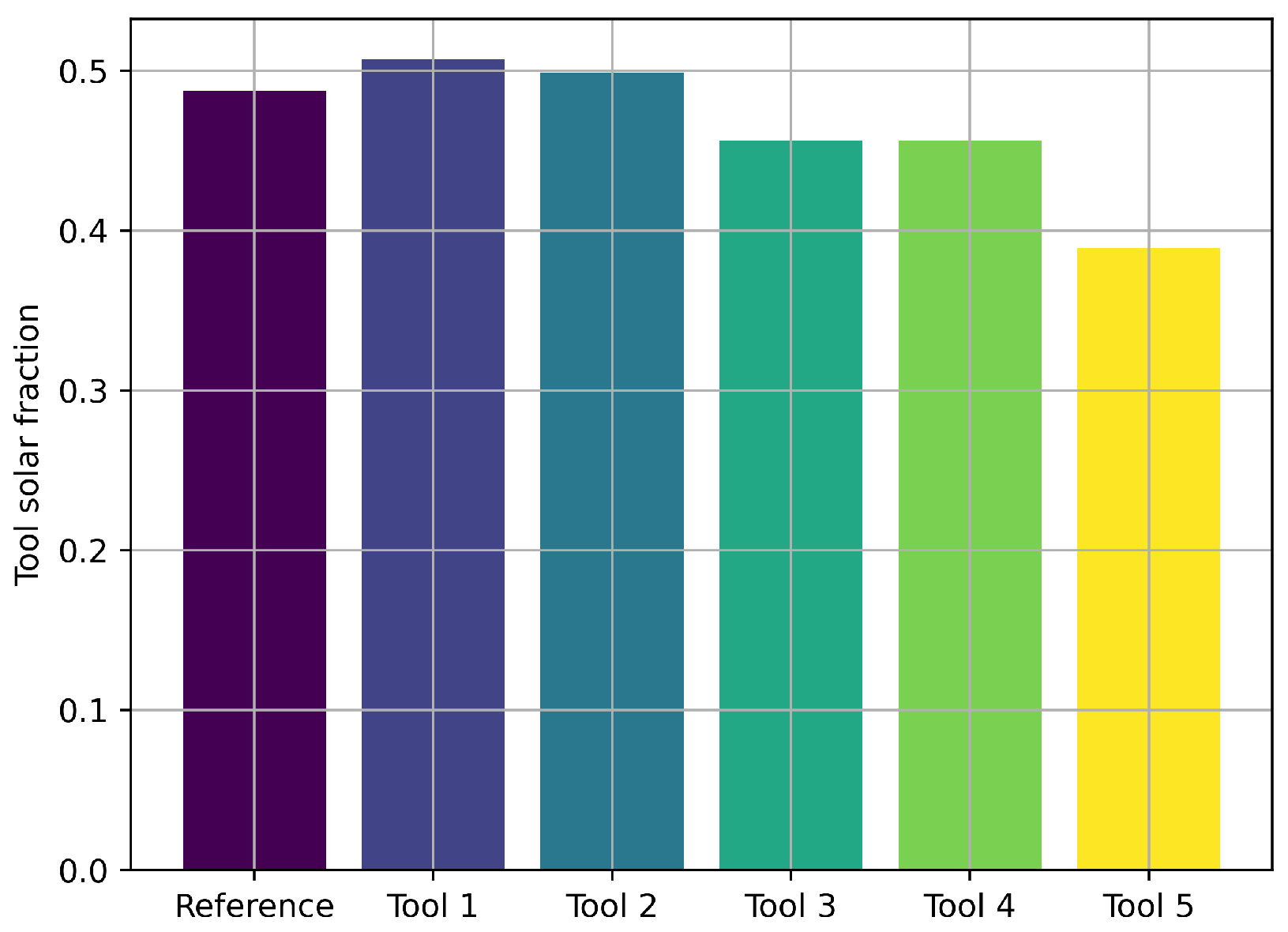
Comparison of Simulation Tools

Different simulation approaches and tools were employed to model the case study system and obtain energy yield results using the same input data. The results were compared to a tool considered as a reference. The reference tool is the one employed in [25], which passed through a validation process considering the public available data of the actual plant. The different simulation tools used for this preliminary assessment were Greenius, Polysun, SAM, the SHIP2FAIR tool, TRNSYS with its basic library and TRNSYS with the TESS library (sorted alphabetically, not necessarily as shown in Figure 4). The results of the solar fraction delivered by the different tools are summarized in Figure 4. In this exercise, the tools are not explicitly assigned to the results, with the aim of avoiding any conflict of interest.

It is observed in Figure 4 that the difference between the yield estimations from different tools can be higher than 10% of the annual solar fraction. Furthermore, when analyzing solar fractions on a monthly and daily basis, the differences can reach about 15% and 20%, as shown in Figure 5a,b, respectively.

As observed, despite the fact that the simulation tools used for the assessment are frequently employed by system developers and researchers, the differences are significantly high, beyond the threshold accepted by the financing industry and/or investors.

4. Scenarios of Induced Errors/Simplifications

The deviations between the simulation results evidenced important differences regarding the simulation approaches, the simplifications that the specialists implemented, and the inherent software’s limitations. By analyzing in detail the results and the documentation of the different software, and validating such information with the analysts, it was possible to identify the main sources of differences, described as follows:

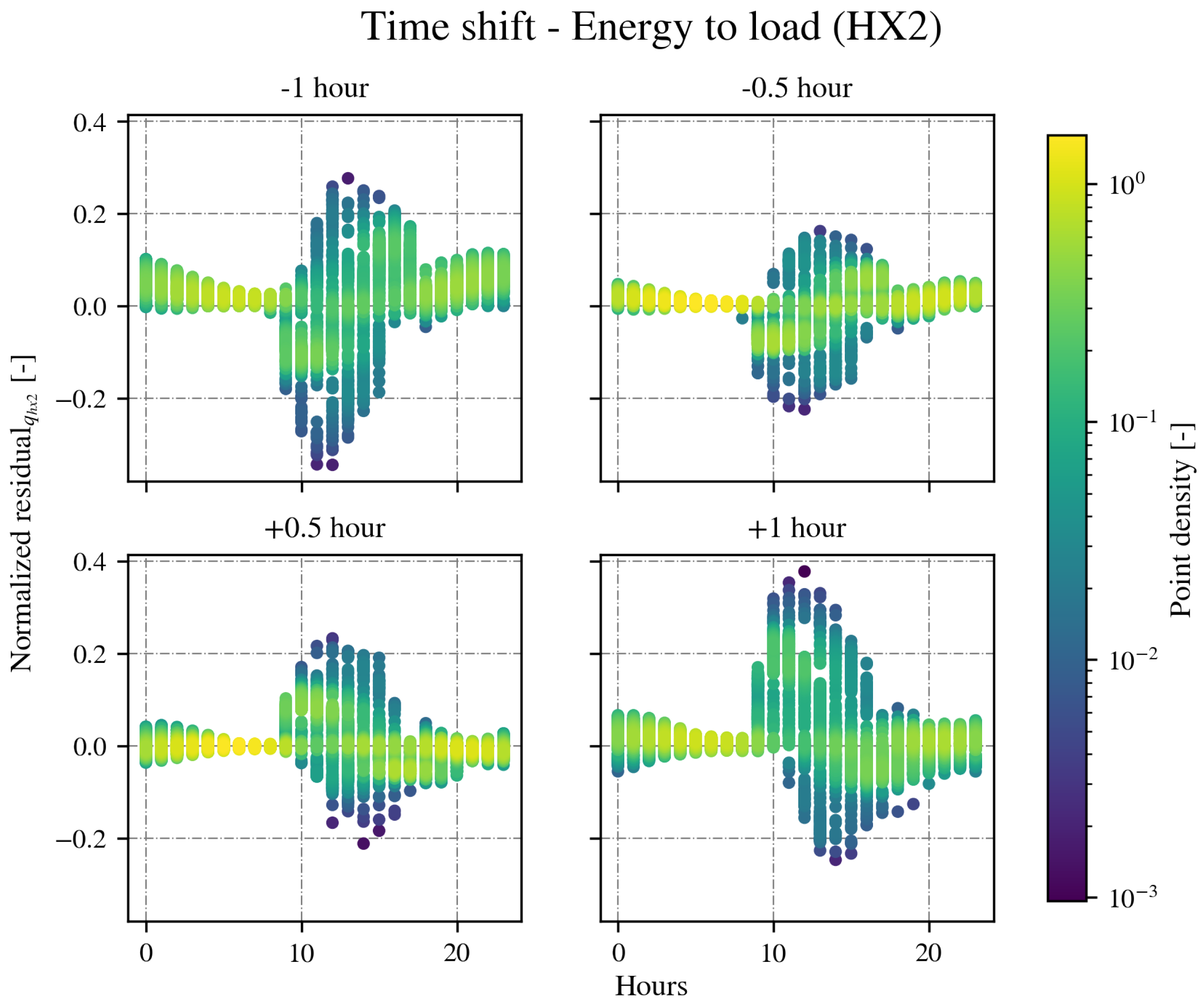
• Time shifting: Most of the simulation tools for solar thermal systems consider hourly radiation data as input, commonly in a TMY format (typical meteorological year format). In that context, the solar radiation is considered constant during the time step reported in the file. In addition, to compute the incident solar radiation on the collector’s plane, it is crucial to have a definition for the solar position during the time step. In this regard, important differences have been observed within the tools analyzed. Certain tools consider the solar position at the beginning of the time step, others at the middle, and others at the end; consequently, they may not agree with the timestamp of the TMY file.
• Thermal capacitance: The thermal capacitance of the solar field is commonly ignored when simulating the performance of SHIP systems. The effect of this simplification is low for small systems; however, it is particularly high in large-scale plants, leading to important deviations in the results of the yield assessment.
• Piping losses: Similarly, piping losses are commonly overlooked when simulating small-scale systems. Nonetheless, in large-scale plants, the length of distribution pipes may increase significantly, thus, the thermal losses also increase, leading to an overestimation of the plant’s energy yield.
• Heat Exchanger modeling: The modeling approach commonly employed for heat exchangers is the consideration of a constant effectiveness. However, determining this parameter depends on information that is not always available. Furthermore, the effectiveness of the heat exchanger may also vary according to the variation of the fluid stream inlets, especially between the heat exchanger coupling the solar field and the TES system. Hence, depending on the proper determination of the effectiveness value and the magnitude of the heat exchanger inlets’ temperature variation, significant deviations can be observed.
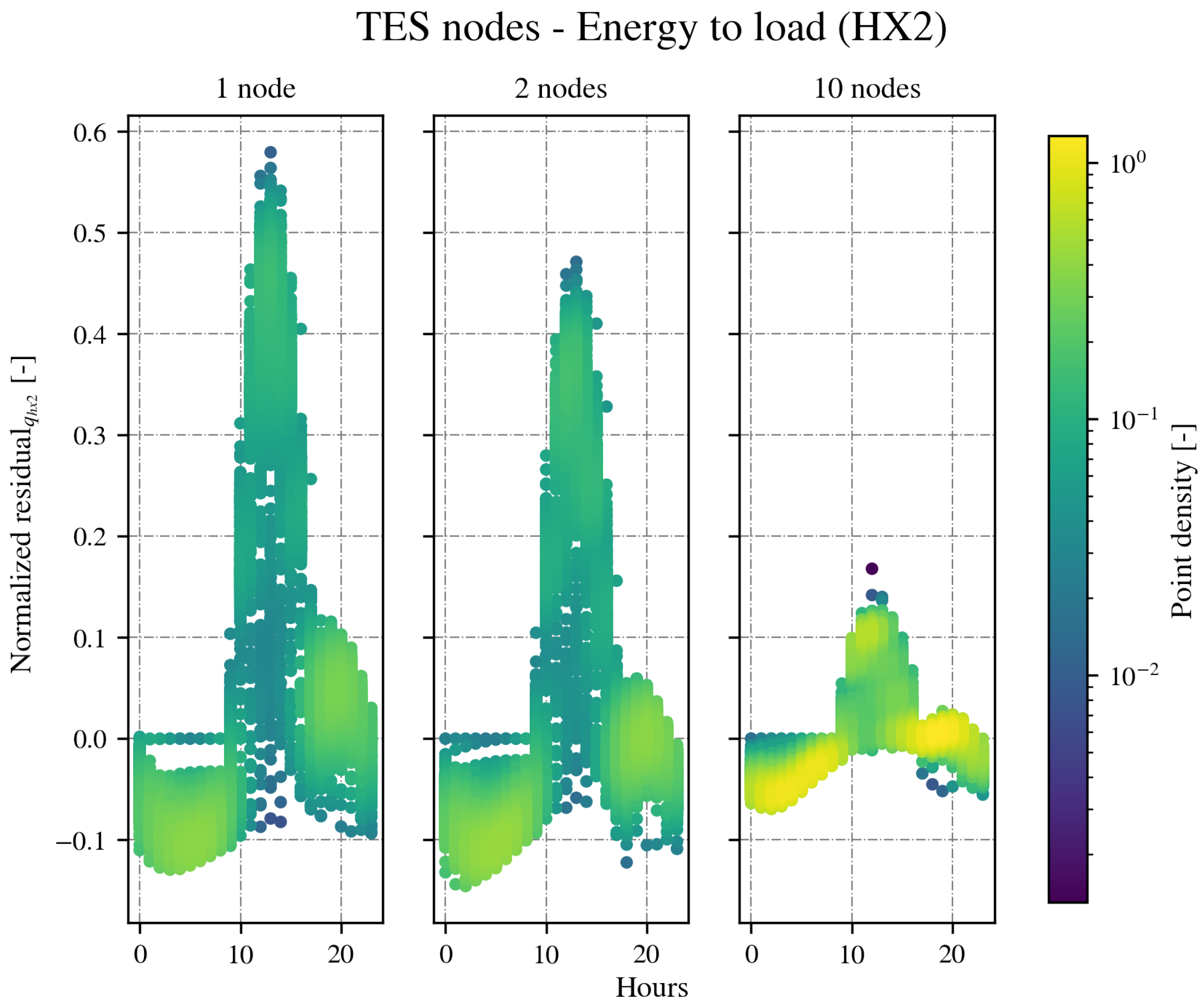
• TES modeling approach: The thermal energy storage (TES) system modeling approach has a large impact on the simulation results. The modeling approach may vary depending on the storage technology; however, in SHIP systems, it is common that the TES corresponds to a stratified liquid tank. To represent the temperature distribution associated with the stratification process, it is common to consider a plug flow modeling strategy, discretizing the storage tank in small volumes. Thus, depending on the number of nodes (volumes) considered, the simulation results may present important deviations. The approaches observed within the simulation tools analyzed range from simple approximations (e.g., 2 nodes) to highly detailed models, considering more than 20 nodes or even solving the differential equations that characterize the natural convection process inside the storage tank.
• Load profile: The definition of the load profile represents an important challenge in the task of constructing the yield assessment of SHIP systems. Usually, there is not enough detailed information to build a detailed load profile, and, thus, it is common to make rough approximations in this regard. To analyze the impact of the load profile on yield estimation, two alternative scenarios are considered based on the standardized load profiles defined in [33].

To address the impact of the different modeling approaches, 20 different simulation scenarios were defined. Subsequently, the results for these scenarios were obtained by employing the reference model and then compared for the analysis. The summary of the scenarios analyzed is depicted in

Table 1. Scenarios of induced errors in simulations.

Source of Deviation	Scenario ID	Time Shifting [h]	Thermal Capacitance [%]	Thermal Insulation (cm)	HX Efectiveness [%]	TES Nodes [-]	Load
Reference	Scenario 0	0	5	5	70	20	Std
Time shifting	Scenario 1	1	5	5	70	20	Std
	Scenario 2	0.5	5	5	70	20	Std
	Scenario 3	−1	5	5	70	20	Std
	Scenario 4	−0.5	5	5	70	20	Std
Thermal capacitance	Scenario 5	0	0.0001	5	70	20	Std
	Scenario 6	0	150	5	70	20	Std
	Scenario 7	0	200	5	70	20	Std
	Scenario 8	0	250	5	70	20	Std
	Scenario 9	0	300	5	70	20	Std
Thermal insulation	Scenario 10	0	5	Underground	70	20	Std
	Scenario 11	0	5	10	70	20	Std
	Scenario 12	0	5	5000	70	20	Std
HX effectiveness	Scenario 13	0	5	5	60	20	Std
	Scenario 14	0	5	5	80	20	Std
	Scenario 15	0	5	5	100	20	Std
TES system	Scenario 16	0	5	5	70	10	Std
	Scenario 17	0	5	5	70	2	Std
	Scenario 18	0	5	5	70	1	Std
Load	Scenario 19	0	5	5	70	20	0–0
	Scenario 20	0	5	5	70	20	2–2

. The simulation of all scenarios was carried out in the TRNSYS software, with the aim of avoiding any bias associated with the software and human factors.

Certain values in Table 1 may seem odd, such as considering 5000 $\mathrm{c}$$\mathrm{m}$ of thermal insulation. The logic behind this is to evaluate the effect of disregarding thermal losses in the model, i.e., perfectly insulated, without modifying the modeling strategy.

5. Methodology for Comparing Time Series from Simulation Tools

The simulation of the scenarios in Table 1 delivers numerical results that are compared using the methodology described in the following sections.

5.1. Statistical Comparison

To configure a flexible methodology for comparing the results of the simulations and to consider the common errors/limitations described in Section 4, a unified open source script for data collection was prepared. It takes into account the hourly, daily, monthly, and annual profiles of the energy delivered and the temperature levels, among other yield parameters. The procedure was programmed in Python using different open-source packages, such as Matplotlib, Pandas, Numpy, SciPy and skillmetrics packages [34,35,36,37]. These packages are useful for data visualization and for reading, processing, postprocessing, and calculating statistical comparison parameters. In addition to that, the Glob and Os packages were used to manipulate file paths.

The differences observed in the comparison between the results profiles of each scenario and the reference are quantified in terms of statistical comparison metrics, such as bias (B), root-mean-square error (RMSE), normalized mean bias error (nMBE), relative difference, pattern root-mean-square difference (RMSD), Pearson correlation coefficient (R), and standard deviation ($\sigma$), which are well-known metrics in statistical analysis and described in depth in [38]. However, only at the hourly level, the RMSD, R and $\sigma$ were correlated within a Taylor diagram to visualize their deviation from the reference case [39]. Therefore, these statistical metrics are defined as follows.

$$B=\overline{y_{est}}-\overline{y_{ref}}$$

(1)

where $y_{est}$ and $y_{ref}$ refer to estimates and reference data sets. Therefore, B represents the bias between these. $\sigma$ is a well known statistical metric defined as follows.

$$\sigma =\sqrt{\frac{{\sum }_{i=1}^N(y_i-\overline{y})}{N-1}}$$

(2)

where $\overline{y}$ and $y_i$ represent the mean and the ith value of the time series analyzed. N is the number of points (length) of the time series analyzed. The correlation coefficient is also a widespread statistical metric, which for the present analysis is defined as

$$R=\frac{COV(y_{est},y_{ref})}{{\sigma }_{y_{est}}·{\sigma }_{y_{ref}}}$$

(3)

$COV(y_{est},y_{ref})$ is the covariance function applied to each scenario and the reference data set.

The normalized Mean Bias Error (nMBE) is defined as follows.

$$\mathrm{nMBE}=\frac{\frac{1}{N}{\sum }_{i=1}^N(y_{est,i}-y_{ref,i})}{Max\left(y_{ref}\right)}$$

(4)

The root mean square error (RMSE), on the other hand, is defined as

$$\mathrm{RMSE}=\sqrt{\frac{1}{N}\sum _{i=1}^N{(y_{est,i}-y_{ref,i})}^2}$$

(5)

The root mean square difference (RMSD) is computed from the $\sigma$ values obtained from the estimated and reference data sets [40].

$$\mathrm{RMSD}=\sqrt{B+{\sigma }_{est}^2+{\sigma }_{ref}^2-2·{\sigma }_{est}^2·{\sigma }_{ref}^2·R}$$

(6)

where ${\sigma }_{est}$ and ${\sigma }_{ref}$ are the standard deviation of the scenario analyzed and the reference, respectively. According to Jolliff et al. [40], if there is no bias between the estimate and the reference data, the RMSD is equivalent to the RMSE.

As shown, for the normalization of MBE the maximum value of the reference data set was used (see Equation (4)); therefore, it represents the increase or decrease of the mean bias associated with this normalization factor. Furthermore, to visualize the effect of variability and outliers on a daily scale, the cumulative distribution functions (CDF) were computed as follows.

$$F_X\left(x\right)=P[X\le x]={\int }_{-\infty }^x{f}_x\left(u\right)du$$

(7)

where for a given value of x, the function $F_X\left(x\right)$ corresponds to the probability that the observed value of X is lower than or equal to x. In addition, the following properties should be considered for the calculation of the CDF:

$$\underset{x\to -\infty }{lim}F\left(x\right)=0and\underset{x\to \infty }{lim}F\left(x\right)=1$$

(8)

if the function $f_x$ is a continuous on x, $P[X\le x]$ corresponds of the derivative of CDF, that is:

$$f_X\left(x\right)=\frac{d{F}_X\left(x\right)}{dx}$$

(9)

According to Arora [41] and Ibe [42], the CDF is used to determine the cumulative probability distribution of a random value or observation x, obtained from the discrete or continuous series to be analyzed, is less than or equal to a certain value. Consequently, one of the main advantages of using a series of data ordered based on its probability of occurrence, is that it offers an ordered visualization platform, which allows us to better differentiate the fit between a reference curve and another curve representing the estimated data. However, the CDF does not allow us to quantify the uncertainty, variability, or precision of the model; therefore, it must be used in conjunction with other statistical metrics. According to Meyer et al. [43] and Espinar et al. [44] the use of three criteria is recommended to quantify the precision of the model in terms of general biases, dispersion, and the ability to reproduce statistical distributions. For such purposes, the recommended metrics are the MBE, RMSE, and the Kolmogorov-Smirnov test (KS) or Kolmogorov-Smirnov integral (KSI) test, respectively [45]. Some authors prefer to replace the use of RMSE with the mean absolute error (MAE); as it is less affected by distant outliers and less subject to interpretation when expressed in comparative terms. Nonetheless, the joint use of the MBE and RMSE provides information on the expected range of errors, offering a better perspective for comparison between simulation tools and a reference.

Although some authors prefer to report the KSI, in the present work, the two-sample KS test was reported at the hourly and daily levels for each control volume. The aim is to identify whether the different scenarios allow us to reproduce the statistical distributions obtained by the reference, with a high degree of confidence [44]. The two-sample KS test assesses the similarity of two data sets through the maximum distance between the CDFs. Although there are several statistical tests to evaluate the goodness of a model, the KS test has the advantage of being a nonparametric and distributionless test. Therefore, this test does not make assumptions about the distribution of data. For this reason, the KS test evaluates the normality and similarity between data sets around the null hypothesis ($H_0$). In fact, the two-sample KS statistic index D is defined as the maximum value of the absolute difference between the two CDFs. Therefore, the KS index can be computed as follows.

$$D=max|CD{F}_{est}\left(X_i\right)-CD{F}_{ref}\left(X_i\right)|$$

(10)

where $CD{F}_{est}\left(X_i\right)$ and $CD{F}_{ref}\left(X_i\right)$ are the CDF data set of the tool to be evaluated and the reference, respectively. The evaluation and analysis of D depend on the level of confidence and the critical value or threshold $V_{c,\alpha }$ below the level of confidence under which the data are evaluated. In general, several authors performed the two-sample KS-test for levels of confidence between 90% and 99.9%. However, to evaluate the goodness of a model or simulation tool, it is recommended to use confidence levels above 95%. Thus, the term $V_{c,\alpha }$ for two samples can be calculated as [46]

$$V_{c,\alpha }=C\left(\alpha \right)\sqrt{\frac{N_1+N_2}{N_1\ast N_2}}$$

(11)

where $N_1$ and $N_2$ are the size of the data set of the tool evaluated and the reference, respectively. The coefficient $C\left(\alpha \right)$ depends on the significance value ($\alpha$), and is generally tabulated for the most used values (

Table 2. $C\left(\alpha \right)$ coefficient concerning the most used significance values for the computed $V_{c,\alpha }$ [46].

Parameter	Values
$\alpha$	0.1	0.05	0.025	0.01	0.005	0.001
$C\left(\alpha \right)$	1.22	1.36	1.48	1.63	1.73	1.95

).

In this way, the null hypothesis $H_0$ can be formulated as follows:

• $H_0$: If D < $V_{c,\alpha }$ the two data sets have a highly similar distribution and could be statistically equivalent. Therefore, the distribution of events and nonevents follows the same sampling distribution.
• Otherwise, $H_0$ must be rejected, and it is considered that the distribution of events and nonevents does not follow the same sampling distribution.

5.2. Hourly Comparison

Determining the differences between time series is an important challenge for comparing simulations of solar thermal systems, since the impacts of the analyst’s assumptions can be recognized. Computing the point-to-point Euclidean distance in this regard, it does not consider the possible shape similarity between two time series as they are not aligned [47]. Typically solar thermal systems are composed of elements with thermal inertia, control schemes, and tracking systems, and their simulation may involve simplifications or assumptions required for the analysis and the simulation tool. Therefore, those characteristics induce a dynamic behavior of the time series, which must be characterized by the proposed methodology for comparison. In that context, two metrics are proposed: the Dynamic Time Warping (DTW) and the dynamics of residuals, which are described in the following sections.

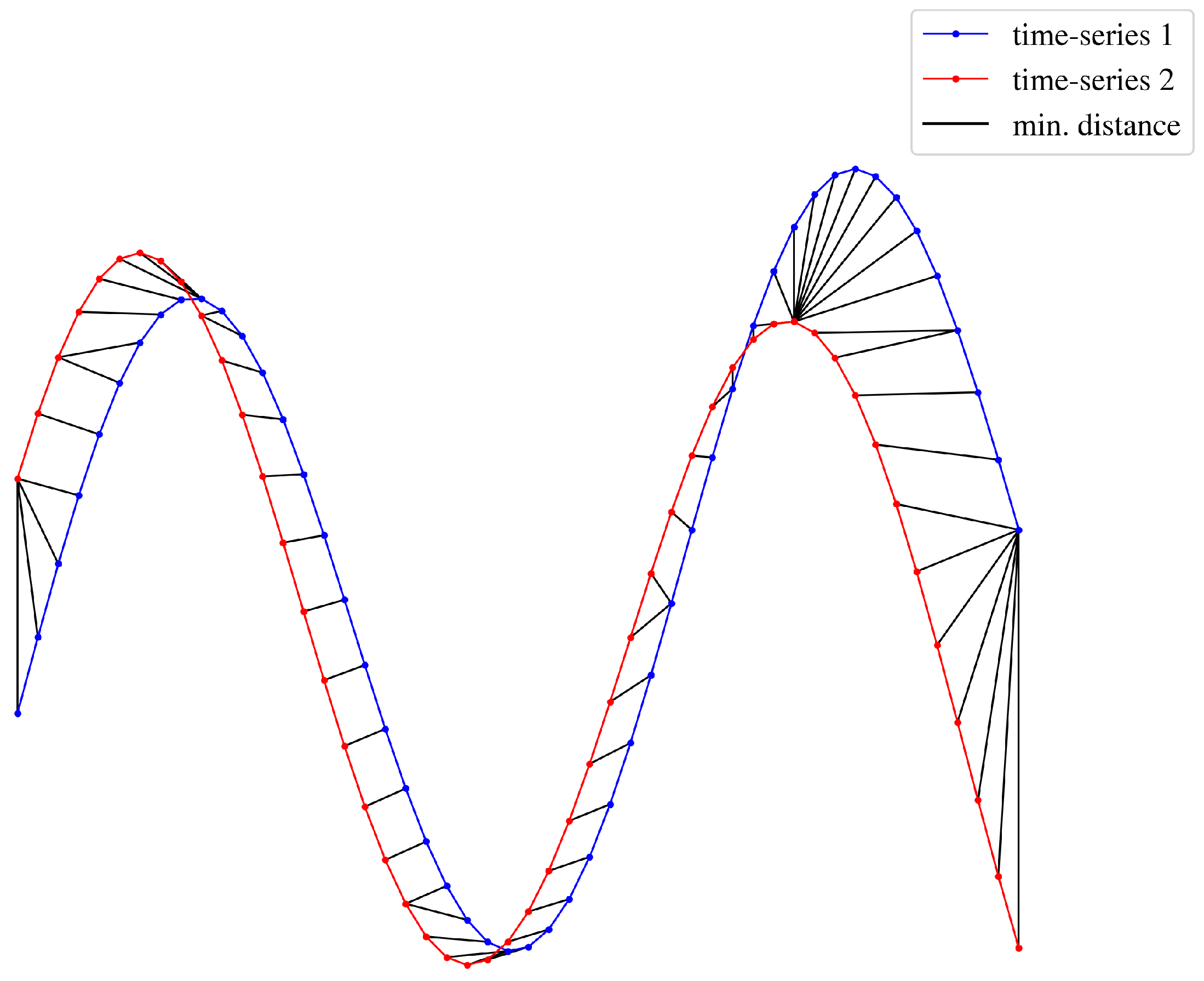
5.2.1. Dynamic Time Warping

The DTW is a technique used for time series analysis, which gives a measure of their similarity by finding the best alignment between them with an associated cost (see Figure 6). Hence, the DTW gives a numerical value that indicates how close one time series in shape and behavior is to another [47,48].

Taking into account two time series X and Y, the cost function c between them is defined as $c:\mathcal{S}\times \mathcal{S}\to \mathbb{R}$. The DTW algorithm aims to minimize c by computing an accumulated distance matrix $\mathcal{D}$. The methodology is summarized in

Table 3. DTW algorithm and construction of accumulated distance matrix.

Given: Time-series $\mathit{\varphi }$ and $\widehat{\mathit{\varphi }}$ of sizes N and M, respectively. Calculate the cost matrix $\mathit{c}=\mathbf{EuclDist}(\mathit{\varphi },\widehat{\mathit{\varphi }})$ with shape $\mathit{N}\times \mathit{M}$.
Given: Cost matrix c. Calculate the accumulated distance matrix $\mathcal{D}$ with the following terms:
Initial value:${\mathcal{D}}_{1,1}={\mathit{c}}_{1,1}$
Boundaries:${\mathcal{D}}_{n,2}={\displaystyle \sum _{i=2}^n}{c}_{i,2}$ for $n=2,\dots ,N$. ${\mathcal{D}}_{2,m}={\displaystyle \sum _{j=2}^m}{c}_{2,j}$ for $m=2,\dots ,M$.
Inner values:${\mathcal{D}}_{n,m}=c_{n,m}+min\left({\mathcal{D}}_{n,m-1},{\mathcal{D}}_{n-1,m},{\mathcal{D}}_{n-1,m-1}\right)$ for $n=2,\dots ,N$ and $m=2,\dots ,M$.
End: The Dynamic Time Warping is the last value of $\mathcal{D}$. $\mathrm{DTW}={\mathcal{D}}_{N,M}$

. In that context, a small value of DTW indicates that X and Y are similar, and a large value if they are different.

The DTW is employed in this study to compare time series on an hourly scale, having a reference simulation $\varphi$ and other simulation of the same system $\widehat{\varphi }$. To visualize the total daily differences, the DTW is calculated for each day of the year with the hourly data of the respective day. In addition to that, the DTW is combined with the Mean Bias Error (MBE) of the day to assess whether the simulation tool underestimates the reference. Considering that there are 8760 values on the hourly scale, the methodology for determining the DTW and MBE values for the two time series is expressed as follows:

• Extract the time series of length 8760 from the reference simulation ($\varphi$) and from the i-th modified simulation (${\widehat{\varphi }}_i$).
• Convert those arrays into matrices of shape $24\times 365$.
• For each day, $d=1,\dots ,365$ determine the value $DT{W}_d(\varphi ,{\widehat{\varphi }}_i)$ and $MB{E}_d=\frac{1}{N_H}{\displaystyle \sum _{i=1}^{N_H}}\left({\varphi }_i-{\widehat{\varphi }}_i\right)$; therefore, the comparison is carried out between the hourly profiles.
• The resulting values are normalized: The DTW is normalized considering the daily demand of the process since it is a cumulative of the dynamic distances between the hourly profiles during the day. The MBE, on the other hand, is normalized by the hourly demand of the process, since it represents an average metric for the hourly values.

The latter step is applied to each simulation tool and compared with the same reference simulation.

5.2.2. Dynamics of Residuals

Although the DTW is useful to determine the impacts that each assumption may cause in the alignment of two time series, it is crucial to determine in the hourly scale whether the simulation is above or below the reference value, i.e., underestimating or overestimating the yield of the SHIP system. Thus, the residual values are calculated by means of the instantaneous difference between the reference and the induced error scenario.

Taking into account instantaneous differences, it is possible to identify the tendency that the modification performs during the day. For instance, if the simulation tends to deliver higher energy values than the reference during the morning and then to underestimate it in the evening. Thus, computing the density of the dataset in an hourly mesh allows us to characterize the distribution of the residuals during the day. Hence, the methodology for computing the proposed analysis is summarized as follows.

• The residual is calculated instantaneously between the reference simulation and the simulation results from the induced error scenario: $\mathrm{res}=\varphi -\widehat{\varphi }$ (1D array of length 8760).
• The objective is to determine the density distribution of the residuals during the day; therefore, the arrays from the previous point must be classified on an hourly scale from hour 0 to 23. Considering that, the Kernel Density Estimation method (KDE) is employed to determine the density distribution of the dataset [49].

According to Chen [49], the KDE can learn the shape of the density from the data, which enables it to be used with complex distributions [49]. This method is already available in the free Python library SciPy [36] as the class gaussian_kde within the module Statistical functions.

Table 4. Summary of the statistical metrics considered.

Metric	Information Provided	Limitations
MBE	Used to capture the average bias in the prediction. Typically used to identify the model’s bias. Furthermore, it indicates the direction of the bias (under- or overestimation).	It is related to the statistical concept of variance, for this reason is prone to outliers as it uses the concept of mean value to calculate each error.
RMSE	Used to measure the error between two data sets. It represents the root of the sum between the variance and the squared bias of an estimated series. It is widely used to study the variability effect on the predictions of a model.	Few large errors in the estimation can produce a significant increase in RMSE. Furthermore, this statistical test does not differentiate between under- or overestimation.
RMSD	Used to obtain the root of the square geometric difference between the dispersion of two data sets, and its correlation with respect to the R value between both series. It is generally used to compare the variability or dispersion between these.	This statistical test does not differentiate between under- or overestimation, and it does not enable us to establish the bias magnitude.
KS	Usually used to compare and study if a model can reproduce the statistical distribution of the reference, evaluating the normality and similarity around the null hypothesis.	This statistical test does not explain the reason of the differences between two data sets. Furthermore, it is focused on evaluating the goodness of the model according the maximum difference in absolute values between the CDFs curves.
DTW	It is employed to measure the similarity between two time series by finding the best alignment among them. The value of the DTW indicates how close in shape is a time series with a reference one.	As it is an improved version of the Euclidean distance, the DTW does not provide information if the series intersect each other.
Dynamic of residuals	Based on the MBE. Thus, this quantity indicates if a simulation instantaneously under- or overestimates the values of a reference simulation.	It does not specify how accurate is the model. Moreover, other sources of errors are not excluded in its formulation.

summarizes the metrics considered for the analysis, indicating the main information provided and the limitations of its application.

6. Results

Figure 7 shows the Taylor diagrams built considering the information from the hourly data for each scenario of induced errors shown in Table 1, and evaluated for the different control volumes of the process: These control volumes are defined as; (a) incident radiation on the SF, (b) solar energy absorbed by the SF, (c) energy delivered to the TES (HX1), and (d) energy delivered to the load (HX2). In Figure 7a it is evidenced that the incident radiation on SF modeled in each scenario presents a good correlation with respect to the reference with values of R above 0.9. Besides that, all tools present standard deviation values similar to the reference time series. Nevertheless, RMSD values show that, despite the good correlation between the time series, there exists a difference in the modeling of this parameter, especially for time-shifting induced errors. The figure shows that for scenarios 1, 2, 3, and 4, there is a loss of adjustment that reaches 6% and an increase in variability with respect to the reference time series between 2500 $\mathrm{kWh}$ and 5000 $\mathrm{kWh}$. Because of that, the deviations induced by time-shifting errors are propagated to the SF’s incident energy computed by the simulation tool. However, despite this, all scenarios present an acceptable correlation.

For the other control volumes of the process, the differences between the simulation results become more evident. The solar energy absorbed by the SF is depicted in Figure 7b). It is observed that the induced errors applied in each scenario propagate errors to the simulation results. Indeed, the induced errors associated with the thermal capacitance, thermal insulation, HX effectiveness, and TES system present the best correlation with the reference in terms of RMSD < 2000 $\mathrm{kWh}$, $\sigma$ less than 9000 $\mathrm{kWh}$, and R-values above 0.96. However, despite that the time-shifting of +1 $\mathrm{h}$ and −1 $\mathrm{h}$ reach $\sigma$ values close to the reference (8000 $\mathrm{kWh}$), there is a loss of adjustment of about 7%. This result implies that the time series modeling within these induced error scenarios presents higher variability with RMSD values of about 3000 $\mathrm{kWh}$, even showing an R-value close to 0.93. Regarding the analysis of the energy delivered to the TES system (HX1) (Figure 7c), it is observed that the induced error scenarios present a similar trend and values in order and magnitude similar to the results shown for the control volume in Figure 7b. The aforementioned is explained by the fact that the energy delivered to the TES system (HX1) is the equivalent of the solar energy absorbed by SF influenced by the piping losses and the efficiency of the HX system assumed in each scenario.

Finally, despite the fact that the TES system reduces the inherent variability of the solar resource, Figure 7d shows that the errors induced by the modeling approach in terms of the nodes considered have a significant impact on the energy dispatched on demand. Within this control volume, the lowest performance in terms of modeling goodness is obtained for a TES system considering 1 (full-mixed) and 2 nodes, which presents a high deviation with respect to the reference. In that context, RMSD values > 1500 $\mathrm{kWh}$ are observed, and an increase of $\sigma$ > 1400 $\mathrm{kWh}$, with an adjustment loss of more than 10%, due to the increase in variability of the reference time series. This is reflected in an R value between 0.79 and 0.85. Therefore, despite the fact that some induced errors show high modeling goodness, the errors introduced at the initial stage of the simulation, such as the errors induced by time-shifting, propagate the deviations over all control volumes in the process.

Figure 8 shows the daily energy profile for the different control volumes of the process. This figure shows the fit with respect to the reference of the different tools and the variability of the simulation results on a daily scale. However, the daily progression does not allow us to properly visualize the effect of outliers, quantify variability, or correctly visualize when a scenario under- or overestimates, or the similarity between the time series. For such purposes, another metric or geometry must be used to make a more reliable comparison.

According to the above-mentioned,

Table A1. Summary of the results obtained trough the CDF analysis.

Control Volume	Scenario	Hourly			Daily
		D	Rejection of ${\mathit{H}}_0$	$(\mathit{D}-{\mathit{V}}_{\mathit{c}})/{\mathit{V}}_{\mathit{c}}$ [%]	D	Rejection of ${\mathit{H}}_0$	$(\mathit{D}-{\mathit{V}}_{\mathit{c}})/{\mathit{V}}_{\mathit{c}}$ [%]
Time Shifting
Incident Radiation on SF	Scenario 1	0.01393	No	−32%	0.09041	No	−10.2%
	Scenario 2	0.01130	No	−45%	0.03014	No	−70.1%
	Scenario 3	0.00925	No	−55%	0.08767	No	−12.9%
	Scenario 4	0.01073	No	−48%	0.03288	No	−67.3%
Absorbed solar energy	Scenario 1	0.00183	No	−91%	0.05753	No	−42.8%
	Scenario 2	0.02968	Yes	44%	0.02740	No	−72.8%
	Scenario 3	0.02477	Yes	21%	0.01918	No	−80.9%
	Scenario 4	0.02511	Yes	22%	0.02740	No	−72.8%
Energy to TES (HX1)	Scenario 1	0.00582	No	−72%	0.05479	No	−45.6%
	Scenario 2	0.02957	Yes	44%	0.02740	No	−72.8%
	Scenario 3	0.01575	No	−23%	0.01370	No	−86.4%
	Scenario 4	0.02215	Yes	8%	0.02740	No	−72.8%
Energy to load (HX2)	Scenario 1	0.00228	No	−89%	0.07123	No	−29.2%
	Scenario 2	0.00011	No	−99%	0.01096	No	−89.1%
	Scenario 3	0.00194	No	−91%	0.04384	No	−56.5%
	Scenario 4	0.00034	No	−98%	0.00822	No	−91.8%
Thermal Capacitance
Incident Radiation on SF	Scenario 5	0	No	−100%	0	No	−100.0%
	Scenario 6	0	No	−100%	0	No	−100.0%
	Scenario 7	0	No	−100%	0	No	−100.0%
	Scenario 8	0	No	−100%	0	No	−100.0%
	Scenario 9	0	No	−100%	0	No	−100.0%
Absorbed solar energy	Scenario 5	0.01256	No	−39%	0.01096	No	−89.1%
	Scenario 6	0.00685	No	−67%	0.01096	No	−89.1%
	Scenario 7	0.01416	No	−31%	0.03836	No	−61.9%
	Scenario 8	0.02192	Yes	7%	0.04658	No	−53.7%
	Scenario 9	0.03037	Yes	48%	0.04384	No	−56.5%
Energy to TES (HX1)	Scenario 5	0.01279	No	−38%	0.01370	No	−86.4%
	Scenario 6	0.00674	No	−67%	0.02740	No	−72.8%
	Scenario 7	0.01438	No	−30%	0.03836	No	−61.9%
	Scenario 8	0.02283	Yes	11%	0.04658	No	−53.7%
	Scenario 9	0.03208	Yes	56%	0.04658	No	−53.7%
Energy to load (HX2)	Scenario 5	0.00080	No	−96%	0.01644	No	−83.7%
	Scenario 6	0.00148	No	−93%	0.01096	No	−89.1%
	Scenario 7	0.00228	No	−89%	0.01918	No	−80.9%
	Scenario 8	0.01336	No	−35%	0.02740	No	−72.8%
	Scenario 9	0.01119	No	−46%	0.02740	No	−72.8%
Thermal Insulation
Incident Radiation on SF	Scenario 10	0	No	−100%	0	No	−100.0%
	Scenario 11	0	No	−100%	0	No	−100.0%
	Scenario 12	0	No	−100%	0	No	−100.0%
Absorbed solar energy	Scenario 10	0	No	−100%	0	No	−100.0%
	Scenario 11	0.00023	No	−99%	0.00274	No	−97.3%
	Scenario 12	0.00046	No	−98%	0.00822	No	−91.8%
Energy to TES (HX1)	Scenario 10	0	No	−100%	0	No	−100.0%
	Scenario 11	0.00046	No	−98%	0.00274	No	−97.3%
	Scenario 12	0.00103	No	−95%	0.00548	No	−94.6%
Energy to load (HX2)	Scenario 10	0	No	−100%	0	No	−100.0%
	Scenario 11	0.00011	No	−99%	0.00274	No	−97.3%
	Scenario 12	0.00034	No	−98%	0.00548	No	−94.6%
HX Effectiveness
Incident Radiation on SF	Scenario 13	0	No	−100%	0	No	−100.0%
	Scenario 14	0	No	−100%	0	No	−100.0%
	Scenario 15	0	No	−100%	0	No	−100.0%
Absorbed solar energy	Scenario 13	0.00114	No	−94%	0.00274	No	−97.3%
	Scenario 14	0.00685	No	−67%	0.00548	No	−94.6%
	Scenario 15	0.00320	No	−84%	0.01096	No	−89.1%
Energy to TES (HX1)	Scenario 13	0.02957	Yes	44%	0.00548	No	−94.6%
	Scenario 14	0.01575	No	−23%	0.00274	No	−97.3%
	Scenario 15	0.02215	Yes	8%	0.01644	No	−83.7%
Energy to load (HX2)	Scenario 13	0.00833	No	−59%	0.03836	No	−61.9%
	Scenario 14	0.00993	No	−52%	0.03014	No	−70.1%
	Scenario 15	0.01347	No	−34%	0.05205	No	−48.3%
TES nodes
Incident Radiation on SF	Scenario 16	0	No	−100%	0	No	−100.0%
	Scenario 17	0	No	−100%	0	No	−100.0%
	Scenario 18	0	No	−100%	0	No	−100.0%
Absorbed solar energy	Scenario 16	0.00639	No	−69%	0.00822	No	−91.8%
	Scenario 17	0.00559	No	−73%	0.01644	No	−83.7%
	Scenario 18	0.02112	Yes	3%	0.05205	No	−48.3%
Energy to TES (HX1)	Scenario 16	0.00342	No	−83%	0.00548	No	−94.6%
	Scenario 17	0.00422	No	−79%	0.01644	No	−83.7%
	Scenario 18	0.02546	Yes	24%	0.05205	No	−48.3%
Energy to load (HX2)	Scenario 16	0.01176	No	−43%	0.00548	No	-94.6%
	Scenario 17	0.19795	Yes	863%	0.13151	Yes	30.6%
	Scenario 18	0.30537	Yes	1386%	0.17534	Yes	74.2%
Load
Incident Radiation on SF	Scenario 19	0	No	−100%	0	No	−100.0%
	Scenario 20	0	No	−100%	0	No	−100.0%
Absorbed solar energy	Scenario 19	0.00126	No	−94%	0.00274	No	−97.3%
	Scenario 20	0.21884	Yes	965%	0.02466	No	−75.5%
Energy to TES (HX1)	Scenario 19	0.00217	No	−89%	0.00274	No	−97.3%
	Scenario 20	0.16233	Yes	690%	0.02740	No	−72.8%
Energy to load (HX2)	Scenario 19	0.12352	Yes	501%	0.09863	No	−2.0%
	Scenario 20	0.10103	Yes	392%	0.21096	Yes	109.6%

shows the results obtained after applying Equations (7)–(11) to all scenarios analyzed (Table 1). The source of deviation related to Time Shifting adds uncertainties to the “Incident Radiation on SF” control volume; however, despite the induced error, the data set can reproduce the statistical distribution of the reference. Furthermore, as shown in the control volumes ‘Absorbed Solar Energy’ and ‘Energy to TES (HX1)’, the uncertainty introduced in the first control volume is transferred to these control volumes, consistent with as shown in Figure 7. Most of the uncertainty introduced is neglected in the “Energy to Load (HX2)” control volume, suggesting that the TES system helps to reduce the uncertainty.

As shown, Thermal Capacitance, Thermal Insulation, HX Effectiveness, TES nodes and Load introduce uncertainties in all control volumes excepting “Incident Radiation on SF”. The TES system helps to reduce the uncertainty introduced, except for the scenario with a low number of TES nodes, which significantly affects the energy delivered to the load. Finally, regarding the load, the uncertainty introduced is due to differences in the load profile with respect to the reference, which even affects the “Absorbed solar energy” control volume due to the plant operation control logic.

In Figure 9 and Figure 10, the daily MBE is plotted against the daily DTW obtained from the hourly profiles, with respect to the energy delivered to the load. According to the methodology described in the previous section, the plots are referred to the scenarios considering different TES modeling approaches and load profiles. Additionally, a colormap is included indicating the day classification (DC), as proposed by Castillejo-Cuberos and Escobar [50], which is a score ranging from 1 (completely overcast day) to 20 (completely cloudless clear day). As observed in Figure 9, there is a linear correlation between the DTW and the MBE values. Moreover, the DTW can reach values up to 12% of the daily demand for a fully mixed tank and a MBE of 10% of the hourly demand. Nevertheless, those values decrease (in modulus) as the TES nodes increase. The latter is due to the modeling approach of the stratification phenomena, since the reference simulation considered 20 nodes to fully characterize the storage tank, fewer nodes induce significant differences in the energy and temperature delivered to the load. It is worth mentioning that the MBE shows negative (energy-to-load overestimated) and positive (energy-to-load underestimated) values during the year. The positive values are mainly associated with clear days, ranging from class 16 to 20 [50]. The negative values, on the other hand, are mainly related to overcast days. In those cases, because of a lack of details regarding the stratification phenomena within the tank, the low temperatures in the TES are overestimated. As a consequence, during the discharge process, the energy delivered to the process is higher than the computed in the reference simulation. In contrast to the effect observed for the different TES modeling approaches, the behavior observed when the demand profiles vary is not significantly affected by the DC index (Figure 10). On the contrary, it is highly dependent on meteorological conditions, such as the solar resource available at the location and ambient temperature (the load profiles are temperature dependent according to [33]. The “v-shape” depicted in Figure 10 indicates that during the process, the daily energy delivered underestimates and overestimates the reference values. In Table A1 the values of the KS test are presented for the different scenarios proposed. According to the KS test, the TES models with 1 and 2 nodes are rejected, while the modeling using 10 nodes is accepted. This behavior is consistent with the dispersion of DTW observed in Figure 9, where using 1 and 2 nodes for modeling the TES system results in errors ranging from 2% to 13% of the normalized DTW, and from 0.2% to 3% when considering the 10 node approach. The same can be deduced from the test of the load profile scenarios and the behavior from Figure 10.

The hourly residuals distributions are presented from Figure 11, Figure 12, Figure 13, Figure 14, Figure 15 and Figure 16, where the point density enables a visualization of whether the induced errors tend to underestimate or overestimate the values of the heat delivered to the load compared to the hourly demand.

• An error in terms of time shifting, i.e., solar position, can induce a difference in the instantaneous heat delivered to the load up to 40% as observed in Figure 11. In this sense, evaluation can lead to errors in rating or sizing some operating systems in the plant, such as control schemes or feedback processes. Another behavior that is interesting to remark is that a +0.5 or +1 h of time shifting overestimates the values during the day and underestimates during the evening. On the other hand, a −0.5 or −1 h presents an inversed impact.
• The effect of thermal capacitance depends on whether the input is lower or larger than the reference. In the first case, there is a tendency on the residuals to be below zero ($q_{hx2}$ overestimated), reaching values higher than the reference up to 10% of the hourly demand. For input values above the reference, during the day the heat to the load is less than the reference, and during the evening it rises. This phenomenon is caused by an increase in the thermal capacity, which is a common behavior obtained due to thermal inertia. In these cases, the reference values are underestimated by 12% of the hourly demand (Figure 12).
• The thermal insulation includes three cases: TES with 10 $\mathrm{c}$$\mathrm{m}$ of insulation, highly insulated (5000 $\mathrm{c}$$\mathrm{m}$ of insulation), and a case where the piping is buried underground. As observed, there are differences in the heat to the load with an amplitude of up to 3% (see Figure 13). Assuming an underground piping does not reflect a high impact on the heat delivered, compared to the reference case, due to the low thermal losses through the piping zones.
• Regarding the heat exchanger modeling approach, the residual distribution for different HX effectiveness scenarios show values lower and higher than the reference (Figure 14). For the values lower than the reference, there is a tendency of increasing the energy delivered to the load during the night and decreasing it during the day. However, there is a higher amplitude in the overestimation as a result of the low value of the effectiveness. For input values of effectiveness larger than the reference, the behavior described is dissimilar. More energy is discharged to the load as there is better heat exchange in the component. In fact, the residuals range from [−5% to 11%], [−10% to 5%] and [−25% to 15%] for the effectiveness of the heat exchanger of 60%, 80%, and 100%, respectively.
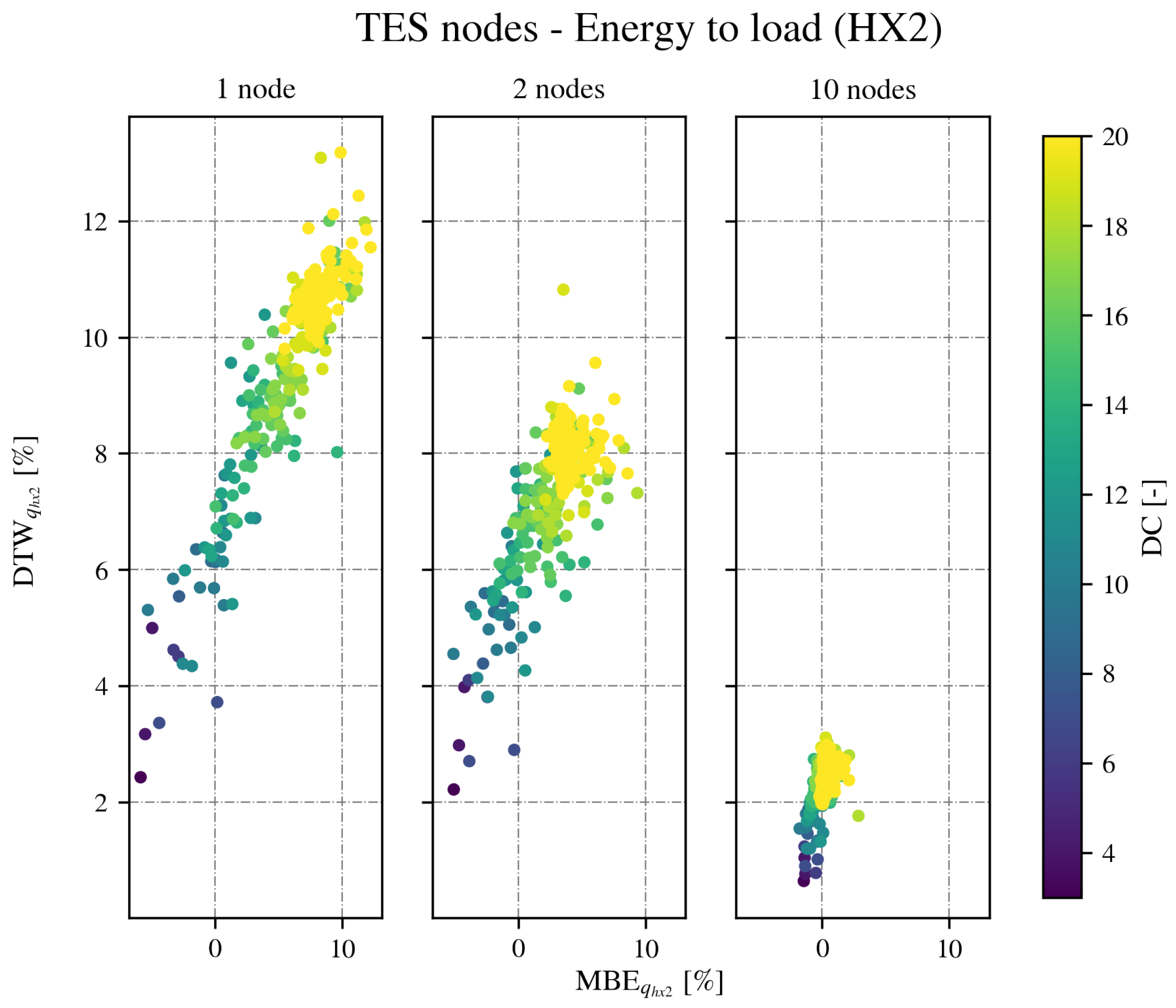
• The distribution of the residuals observed for the TES modeling induced errors are assessed considering scenarios with different numbers of nodes in the numerical model of the TES. The assessment considers ranging the TES nodes between 20 (reference), 10, 2, and 1 (full-mixed), as illustrated in Figure 15. The effect observed corresponds to an increase in the amplitude of the residual values as the TES nodes decrease. During hours with no solar radiation available, the heat delivered to the load is overestimated, because of the lack of stratification in the system. Hence, higher temperatures can be achieved in the discharging process of the TES as there are fewer nodes to interpolate to model the thermocline. Furthermore, a full mixed tank can underestimate the energy delivered to the load during the day by 50% of the hourly demand. Finally, despite having low values of DTW, using 10 nodes for modeling, stratification of TES underestimates the heat delivered to the process by 10% during the day.
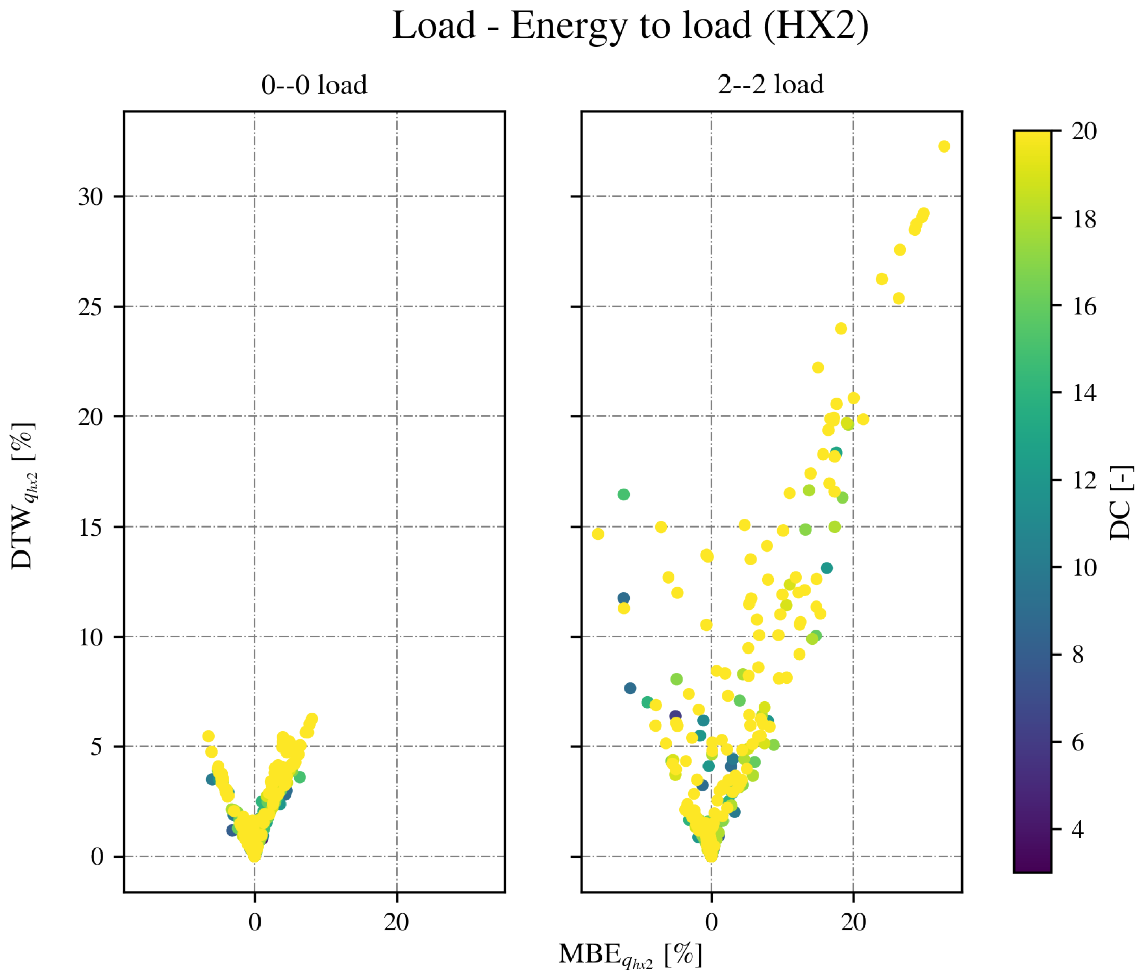
• Considering a variable load profile dependent on the mean daily temperature of the surroundings is assessed though two scenarios: Case 0-0, which corresponds to an approximately constant demand during the week. In the left plot of Figure 16, it is observed that the values are concentrated in zero residuals, but with hourly variations up to 20% of the hourly demand. That behavior is caused by the seasonal variation in the temperature of the surroundings. Hence, the demand will also vary, affecting the heat delivered to the process. The case 2-2 corresponds to an extreme case where a significant difference in demand is observed between the working days and the weekend. The resulting variation of the residuals is of a similar shape to the case 0-0. Nonetheless, a higher amplitude is observed in the differences. In Figure 16 a maximum of 65% of the hourly demand is reached. Overall, the distribution indicates that with a temperature-dependent demand, during the early morning hours, the heat delivered is overestimated and then until 10 pm is underestimated.

In Figure 17 the difference in terms of solar fraction between the reference case and each induced error scenario: $\Delta SF=S{F}_c-S{F}_{ref}$ is shown. Thus, this figure can be used to identify the impact of the analyzed parameters on the annual solar fraction.

Taking into account the effects of each induced error scenario, the thermal insulation thickness employed and the consideration of the piping losses do not represent a significant impact on the solar fraction estimated for the system, since the overall losses are almost negligible, compared to the large energy demand considered for the case study. Furthermore, taking into consideration the dynamic distribution of the residuals (Figure 13) it is demonstrated that the small instantaneous differences do not significantly impact the estimation of the solar fraction. On the other hand, the time shifting, the number of TES nodes, and the load profile induced error causes a underestimation of the solar fraction. The first is due to the miscalculation of the total energy delivered by the solar field. The offset in the sun’s position causes a decrease on the energy provided each day and the solar fraction experiments an reduction of 3%, depending on the size of the time shifting (Figure 17). Regarding the TES modeling (number of nodes), in all cases the solar fraction estimated is lower than the reference due to a linearization of the stratification effect; therefore, using fewer nodes leads to an important underestimation of the temperature achieved within the tank. Implementing a variable load profile leads to a reduction on the solar fraction estimated (Figure 17) because of its dependency on the daily mean temperature of the surroundings and in different scenarios regarding the energy delivered during the weekend. The solar fraction values are expected to be underestimated as the energy required during the morning and afternoon is lower than the reference case (Figure 16).

A thermal capacitance in the solar field lower than the reference value leads to an overestimation of the solar fraction, as part of the heat accumulated in the equipment is disregarded and assumed to be transferred completely to the process. In cases where the thermal capacity is larger than the reference value, there is a higher amount of heat contained in the solar field and less energy provided to the process. This dynamic behavior impacts the solar fraction and can be overestimated by 1% or underestimated by 2% depending on the thermal capacitance, as observed in Figure 17. The assumption of the value considered for the HX effectiveness affects the solar fraction in a contrary way. For lower values, the solar fraction decreases, as the energy transferred is lower. Whereas in cases considering higher HX effectiveness, the solar fraction increases (Figure 17).

7. Discussion

This section presents a discussion of the main outcomes of this study. It is divided in three primary subjects: the observations of the raw results obtained by different simulation tools and analysts, the findings observed from the quantitative comparison, and the scope of this study and its limitations.

The raw results obtained from the different simulation tools for the case study were examined individually to check the coherence of the data and the expected seasonal behavior. Figure 4 and Figure 5a present the annual, monthly, and daily solar fractions estimated by all the tools analyzed. However, the comparison was also performed for the intermediate control volumes and hourly values, where the differences observed led to the development of the induced error scenarios. For instance, when there were differences in the heat supplied to the TES at the start of the day, the time shifting in the radiation data and capacitance of the solar field and other components were identified as causes. In addition, when tools with similar sky model and radiation processors noticeably differed in the energy losses between the solar field and the TES system, the thermal losses in the piping and HX modeling approaches were identified as sources of the differences. In addition, when the TES output temperature and the energy delivered to the load on an hourly basis were observed, the impact of the TES stratification level was detected.

Furthermore, the results comparison employing statistic metrics addressed the quantification of the impact of the uncertainty sources. First, commonly employed statistic metrics such as standard deviation, nRMSD, nMBE, and Pearson’s correlation coefficient were used for annual, monthly, and daily values. However, these metrics are not suitable for directly comparing the hourly values of time series. Therefore, the dynamic time warping (DTW) is employed and the residual distribution is calculated and plotted for hourly values. This approach allows us to identify the tendencies of under- or overestimation of the energy flows and the time of the day when they occur.

Finally, it is necessary to note that this stage of the IEA SHC Task64/SolarPACES task IV—Subtask C, and particularly this study, aims to identify and classify the uncertainty sources from different simulation tools. Therefore, only results from simulation models were compared, and real operation data were not included in the analysis. However, a comparison with actual operational data is expected in the next stages. In the present study, there are certain limitations that can be separated into information exchange constraints and methodology limitations. The first is related to a misunderstanding of certain plant configuration parameters or the format of the output file by the analyst. For example, the method employed to introduce some parameters or coefficients into the simulation tools, since not all tools allow us to receive the input information in the same format. It is relevant to bear in mind that the simulation models were developed by different analysts from different countries, where the information was submitted remotely. Therefore, to avoid errors due to information misunderstanding, bilateral meetings were held between the core team and the different analysts to clarify doubts and receive comments.

Regarding the limitations of the methodology, a key factor for time-dependent simulations is the definition of a suitable simulation time step. Since solar thermal systems have thermal inertia due to the materials and the fluid in the circuits, the system’s response speed might be different than the simulation time step. Therefore, it is worthwhile to estimate the time constant of the real system, commonly defined as $\tau$, and employ a simulation time step of the same order of magnitude to allow the controller to make decisions with reliable variable magnitudes. The time constant describes the speed with which the measured process variable responds to changes in the controller output for a first-order control system. Specifically, the time that the variable takes to reach 63.2% of its final value when a step input is applied [51]. Nevertheless, since the time step cannot be modified in certain simulation software and the most frequent time step employed in the solar thermal sector for annual simulations is 1 h, this time step was employed for the maximum time resolution in the analysis. Furthermore, the inherent limitations of each simulation tool for representing solar thermal systems (such as numerical solver, number of allowable iterations, among others) have not been explicitly considered in the analysis since they are out of the control of the user. However, it was then identified that they might impact the uncertainty of the output, e.g., the energy yield.

8. Conclusions

The present study describes a methodology approach for assessing the impact of common assumptions applied in yield assessment of SHIP systems. In this context, it was defined as a case study based on the general features of an actual plant. The methodology proposed allowed us to identify the main sources of differences among the simulation tools used for yield assessment in SHIP systems. Based on the sources of deviation identified, a statistical assessment of the deviation was implemented, considering a series of statistical metrics selected for such purposes.

The analysis carried out allowed us to quantify the errors in different time scales, identifying the limitations and the BIAS of considering an analysis based on a single time scale. In the next stages of this initiative, the size of the system should be considered, as well as the impact of the time constant of the subsystems and the solver utilized by the simulation tool.

Although the sources of deviation might be considered as predictable, through the methodology presented herein, it is possible to determine the magnitude of the deviations associated with the induced errors. Hence, the results obtained constitute an important contribution to the solar community, allowing us to build a guideline for developing a yield assessment with known uncertainties associated with the simulation approach or software limitations. By creating a common framework for building yield assessment of solar thermal systems, it might be possible to partially reduce the risk perceived by the financing industry regarding SHIP systems. Thus, the methodology developed herein and the information collected through the proposed methodology could contribute significantly to fostering the deployment of SHIP systems.

References

1. IEA. Key World Energy Statistics; Technical Report August; International Energy Agency: Paris, France, 2020. [Google Scholar]
2. Farjana, S.H.; Huda, N.; Mahmud, M.A.P.; Saidur, R. Solar process heat in industrial systems—A global review. Renew. Sustain. Energy Rev. 2018, 82, 2270–2286. [Google Scholar] [CrossRef] [Green Version]
3. IRENA-ETSAP. Solar Heat for Industrial Processes; Technical Report Technology Brief—21; IRENA: Abu Dhabi, United Arab Emirates, 2015. [Google Scholar]
4. Tabassum, S.; Rahman, T.; Islam, A.U.; Rahman, S.; Dipta, D.R.; Roy, S.; Mohammad, N.; Nawar, N.; Hossain, E. Solar Energy in the United States: Development, Challenges and Future Prospects. Energies 2022, 4, 8142. [Google Scholar] [CrossRef]
5. IEA. Tracking Industry 2020. Available online: https://www.iea.org/reports/tracking-industry-2020 (accessed on 25 October 2021).
6. Tasmin, N.; Farjana, S.H.; Hossain, M.R.; Golder, S.; Parvez Mahmud, M.A. Integration of Solar Process Heat in Industries: A Review. Clean Technol. 2022, 4, 97–131. [Google Scholar] [CrossRef]
7. Sharma, A.K.; Sharma, C.; Mullick, S.C.; Kandpal, T.C. Solar industrial process heating: A review. Renew. Sustain. Energy Rev. 2017, 78, 124–137. [Google Scholar] [CrossRef]
8. Kurup, P.; Zhu, G.; Turchi, C.S. Solar process heat potential in California, USA. In Proceedings of the EuroSun 2016; International Solar Energy Society: Freiburg, Germany, 2016. [Google Scholar]
9. Schoeneberger, C.A.; McMillan, C.A.; Kurup, P.; Akar, S.; Margolis, R.; Masanet, E. Solar for industrial process heat: A review of technologies, analysis approaches, and potential applications in the United States. Energy 2020, 206, 118083. [Google Scholar] [CrossRef]
10. Guillaume, M.; Bunea, M.S.; Caflisch, M.; Rittmann-Frank, M.H.; Martin, J. Solar heat in industrial processes in Switzerland: Theoretical potential and promising sectors. In Proceedings of the EuroSun 2018; International Solar Energy Society: Freiburg, Germany, 2018. [Google Scholar]
11. Farjana, S.H.; Huda, N.; Mahmud, M.A.P.; Saidur, R. Solar industrial process heating systems in operation—Current SHIP plants and future prospects in Australia. Renew. Sustain. Energy Rev. 2018, 91, 409–419. [Google Scholar] [CrossRef] [Green Version]
12. Jia, T.; Huang, J.; Li, R.; He, P.; Dai, Y. Status and prospect of solar heat for industrial processes in China. Renew. Sustain. Energy Rev. 2018, 90, 475–489. [Google Scholar] [CrossRef] [Green Version]
13. Fluch, J.; Gruber-Glatzl, W.; Brunner, C.; Shrestha, S.; Sayer, M. Solar heat for industrial processes in Malaysia and Egypt. In Proceedings of the ISES Solar World Congress 2019; International Solar Energy Society: Freiburg, Germany, 2019. [Google Scholar]
14. Weiss, W.; Spörk-Dür, M. Solar-Heat-Worldwide 2020; Technical Report; IEA—Solar Heating and Cooling Programme: Paris, France, 2020. [Google Scholar]
15. Brunner, C.; Giannakopoulou, B.S.K.; Schnitzer, H. Industrial Process Indicators and Heat Integration in Industries; Technical Report Task 33/IV “Solar Heat for Industrial Processes“; IEA SHC/SolarPACES: Paris, France, 2008. [Google Scholar]
16. Pierre Krummenacher, B.M. Methodologies and Software Tools for Integrating Solar Heat into Industrial Processes; Technical Report IEA Task 49/IV—Deliverable B1; IEA SHC/SolarPACES: Paris, France, 2015. [Google Scholar]
17. Guisado, M.V.; Zaversky, F.; Bernardos, A.; Santana, I. Solar heat for industrial processes (ship): Modeling and optimization of a parabolic trough plant with thermocline thermal storage system to supply medium temperature process heat. In Proceedings of the EuroSun 2016; International Solar Energy Society: Freiburg, Germany, 2016. [Google Scholar]
18. Desideri, A.; Dickes, R.; Bonilla, J.; Valenzuela, L.; Quoilin, S.; Lemort, V. Steady-state and dynamic validation of a parabolic trough collector model using the ThermoCycle Modelica library. Sol. Energy 2018, 174, 866–877. [Google Scholar] [CrossRef]
19. Bolognese, M.; Viesi, D.; Bartali, R.; Crema, L. Modeling study for low-carbon industrial processes integrating solar thermal technologies. A case study in the Italian Alps: The Felicetti Pasta Factory. Sol. Energy 2020, 208, 548–558. [Google Scholar] [CrossRef]
20. Frasquet, M. SHIPcal: Solar Heat for Industrial Processes Online Calculator. Energy Procedia 2016, 91, 611–619. [Google Scholar] [CrossRef] [Green Version]
21. Frasquet, M.; Bannenberg, J.; Silva, M.; Nel, Y. RESSSPI: The network of simulated solar systems for industrial processes. In Proceedings of the EuroSun 2018; International Solar Energy Society: Freiburg, Germany, 2018. [Google Scholar]
22. Muster, B.; Ben Hassine, I.; Helmke, A.; Heß, S.; Krummenacher, P.; Schmitt, B.; Schnitzer, H. Integration Guideline; Technical Report Task 49—Deliverable B2; IEA SHC/SolarPACES: Paris, France, 2015. [Google Scholar]
23. Klein, S.A. A Transient Systems Simulation Program; Version 18.00.0019; TRNSYS: Madison, WI, USA, 2018. [Google Scholar]
24. Lugo, S.; García-Valladares, O.; Best, R.; Hernández, J.; Hernández, F. Numerical simulation and experimental validation of an evacuated solar collector heating system with gas boiler backup for industrial process heating in warm climates. Renew. Energy 2019, 139, 1120–1132. [Google Scholar] [CrossRef]
25. Quiñones, G.; Felbol, C.; Valenzuela, C.; Cardemil, J.M.; Escobar, R.A. Analyzing the potential for solar thermal energy utilization in the Chilean copper mining industry. Sol. Energy 2020, 197, 292–310. [Google Scholar] [CrossRef]
26. Crespo, A.; Muñoz, I.; Platzer, W.; Ibarra, M. Integration enhancements of a solar parabolic trough system in a Chilean juice industry: Methodology and case study. Sol. Energy 2021, 224, 593–606. [Google Scholar] [CrossRef]
27. Blair, N.; Dobos, A.P.; Freeman, J.; Neises, T.; Wagner, M. System Advisor Model, SAM 2014.1.14: General Description; Technical Report NREL/TP-6A20-61019; National Renewable Energy Laboratory: Golden, CO, USA, 2014. [Google Scholar]
28. Kurup, P.; Parikh, A.; Möllenkamp, J.; Beikircher, T.; Samoli, A.; Turchi, C. SAM process heat model development and validation: Liquid-HTF trough and direct steam generation linear focus systems. In Proceedings of the SWC2017/SHC2017; International Solar Energy Society: Freiburg, Germany, 2017. [Google Scholar]
29. Kurup, P.; Turchi, C. Case study of a Californian brewery to potentially use concentrating solar power for renewable heat generation. In Proceedings of the ISES Solar World Congress 2019; International Solar Energy Society: Freiburg, Germany, 2019. [Google Scholar]
30. Suresh, N.S.; Rao, B.S. Solar energy for process heating: A case study of select Indian industries. J. Clean. Prod. 2017, 151, 439–451. [Google Scholar] [CrossRef] [Green Version]
31. Eddouibi, J.; Abderafi, S.; Vaudreuil, S.; Bounahmidi, T. Dynamic simulation of solar-powered ORC using open-source tools: A case study combining SAM and coolprop via Python. Energy 2022, 239, 121935. [Google Scholar] [CrossRef]
32. IEA/SHC. IEA-SHC Programme—Task 64: Solar Process Heat. 2021. Available online: https://task64.iea-shc.org/ (accessed on 16 December 2021).
33. Jesper, M.; Pag, F.; Vajen, K.; Jordan, U. Annual Industrial and Commercial Heat Load Profiles: Modeling Based on k-Means Clustering and Regression Analysis. Energy Convers. Manag. X 2021, 10, 100085. [Google Scholar] [CrossRef]
34. Hunter, J.D. Matplotlib: A 2D Graphics Environment. Comput. Sci. Eng. 2007, 9, 90–95. [Google Scholar] [CrossRef]
35. Wes McKinney. Data Structures for Statistical Computing in Python. In Proceedings of the 9th Python in Science Conference, 28 June–3 July 2010; Austin, TX, USA; pp. 56–61. [CrossRef] [Green Version]
36. Virtanen, P.; Gommers, R.; Oliphant, T.E.; Haberland, M.; Reddy, T.; Cournapeau, D.; Burovski, E.; Peterson, P.; Weckesser, W.; Bright, J.; et al. SciPy 1.0: Fundamental Algorithms for Scientific Computing in Python. Nat. Methods 2020, 17, 261–272. [Google Scholar] [CrossRef] [Green Version]
37. Harris, C.R.; Millman, K.J.; van der Walt, S.J.; Gommers, R.; Virtanen, P.; Cournapeau, D.; Wieser, E.; Taylor, J.; Berg, S.; Smith, N.J.; et al. Array programming with NumPy. Nature 2020, 585, 357–362. [Google Scholar] [CrossRef]
38. Pal, R. Chapter 4—Validation methodologies. In Predictive Modeling of Drug Sensitivity; Pal, R., Ed.; Academic Press: Cambridge, MA, USA, 2017; pp. 83–107. [Google Scholar] [CrossRef]
39. Yearsley, J.R.; Sun, N.; Baptiste, M.; Nijssen, B. Assessing the impacts of hydrologic and land use alterations on water temperature in the Farmington River basin in Connecticut. Hydrol. Earth Syst. Sci. 2019, 23, 4491–4508. [Google Scholar] [CrossRef] [Green Version]
40. Jolliff, J.K.; Kindle, J.C.; Shulman, I.; Penta, B.; Friedrichs, M.A.; Helber, R.; Arnone, R.A. Summary diagrams for coupled hydrodynamic-ecosystem model skill assessment. J. Mar. Syst. 2009, 76, 64–82. [Google Scholar] [CrossRef]
41. Arora, J.S. Chapter 20—Additional Topics on Optimum Design. In Introduction to Optimum Design, 3rd ed.; Arora, J.S., Ed.; Academic Press: Boston, MA, USA, 2012; pp. 731–784. [Google Scholar] [CrossRef]
42. Ibe, O.C. Chapter 2—Random Variables. In Fundamentals of Applied Probability and Random Processes, 2nd ed.; Ibe, O.C., Ed.; Academic Press: Boston, MA, USA, 2014; pp. 57–79. [Google Scholar] [CrossRef]
43. Meyer, R.; Schlecht, M.; Chhatbar, K.; Weber, S. Chapter 3—Solar resources for concentrating solar power systems. In Concentrating Solar Power Technology, 2nd ed.; Lovegrove, K., Stein, W., Eds.; Woodhead Publishing Series in Energy; Woodhead Publishing: Cambridge, UK, 2021; pp. 73–98. [Google Scholar] [CrossRef]
44. Espinar, B.; Ramírez, L.; Drews, A.; Beyer, H.G.; Zarzalejo, L.F.; Polo, J.; Martín, L. Analysis of different comparison parameters applied to solar radiation data from satellite and German radiometric stations. Sol. Energy 2009, 83, 118–125. [Google Scholar] [CrossRef]
45. Perez, R.; Cebecauer, T.; Šúri, M. Chapter 2—Semi-Empirical Satellite Models. In Solar Energy Forecasting and Resource Assessment; Kleissl, J., Ed.; Academic Press: Boston, MA, USA, 2013; pp. 21–48. [Google Scholar] [CrossRef]
46. Riffenburgh, R.H. Chapter 20—Tests on the Distribution Shape of Continuous Data. In Statistics in Medicine, 2nd ed.; Riffenburgh, R.H., Ed.; Academic Press: Burlington, MA, USA, 2006; pp. 369–386. [Google Scholar] [CrossRef]
47. Keogh, E.J.; Pazzani, M.J. Derivative Dynamic Time Warping. In Proceedings of the 2001 SIAM International Conference on Data Mining (SDM), Chicago, IL, USA, 5–7 April 2001; Society for Industrial and Applied Mathematics: Philadelphia, PA, USA, 2001; pp. 1–11. [Google Scholar] [CrossRef] [Green Version]
48. Petitjean, F.; Ketterlin, A.; Gançarski, P. A global averaging method for dynamic time warping, with applications to clustering. Pattern Recognit. 2011, 44, 678–693. [Google Scholar] [CrossRef]
49. Chen, Y.C. A tutorial on kernel density estimation and recent advances. Biostat. Epidemiol. 2017, 1, 161–187. [Google Scholar] [CrossRef]
50. Castillejo-Cuberos, A.; Escobar, R. Understanding solar resource variability: An in-depth analysis, using Chile as a case of study. Renew. Sustain. Energy Rev. 2020, 120, 109664. [Google Scholar] [CrossRef]
51. Liptak, B.G. Instrument Engineers’ Handbook, Volume Two: Process Control and Optimization; CRC Press: Boca Raton, FL, USA, 2018. [Google Scholar]
Figure 1. Methodology implemented to identify the sources of differences in the results of energy yield assessments employing different simulation tools (software).
Energies 15 03333 g001
Figure 2. IAM coefficients for the Flat Plate collectors.
Energies 15 03333 g002
Figure 3. System diagram of the case study: flat plate collectors solar field coupled to a copper mining process.
Energies 15 03333 g003
Figure 4. Annual solar fraction calculated by the different tools.
Energies 15 03333 g004
Figure 5. Differences between the different simulation tools in terms of the Solar Fraction.
Energies 15 03333 g005
Figure 6. Scheme of DTW distances between two time-series.
Energies 15 03333 g006
Figure 7. Taylor diagrams of (a) incident radiation on SF, (b) absorbed solar energy by SF, (c) energy delivered to TES (HX1), and (d) energy delivered to load (HX2) obtained through hourly data.
Energies 15 03333 g007
Figure 8. Progression of the daily totals for the different process’s control volumes.
Energies 15 03333 g008
Figure 9. Relationship between the daily DTW and MBE for different classification days for variation in TES nodes.
Energies 15 03333 g009
Figure 10. Relationship between the daily DTW and MBE for different classification days for variation in the load profiles.
Energies 15 03333 g010
Figure 11. Residuals distribution for the time shifting error scenarios.
Energies 15 03333 g011
Figure 12. Residuals distribution for thermal capacitance error scenarios.
Energies 15 03333 g012
Figure 13. Residuals distribution for thermal insulation induced error scenarios.
Energies 15 03333 g013
Figure 14. Residuals distribution for induced error scenarios regarding HX effectiveness.
Energies 15 03333 g014
Figure 15. Residuals distribution for the induced scenarios regarding the TES modeling approach.
Energies 15 03333 g015
Figure 16. Residuals distribution for different load profiles scenarios.
Energies 15 03333 g016
Figure 17. Difference between the reference solar fraction and the induced modification.
Energies 15 03333 g017