A CFD Modelling Approach for the Operation Analysis of an Exhaust Backpressure Valve Used in a Euro 6 Diesel Engine

Abstract

Harvesting residual thermal energy from exhaust gases with thermoelectric generators is one of the paths that are currently being explored to achieve more sustainable and environmentally friendly means of transport. In some cases, thermoelectric generators are installed in a by-pass configuration to regulate the mass flow entering the thermoelectric generator. Some manufacturers are using throttle valves with electromechanical actuators and electronic control in the exhaust pipe to improve techniques for active control of pollutant emissions in reciprocating internal combustion engines, such as the exhaust gas recirculation. The above-mentioned circumstances have motivated the approach of this work: computational fluid dynamics (CFD) modelling of the operation of a throttle valve used for establishing adequate exhaust backpressure conditions to achieve the low pressure exhaust gas recirculation in Euro 6 engines. The aim of this model is to understand the flow control process with these types of valves in order to incorporate them in an exhaust system that will include two thermoelectric generators used to convert residual thermal energy into electrical energy. This work presents a computational model of the flow through the throttle valve under different temperatures and mass flow rates of the exhaust gas with different closing positions. For all cases, the values of the pressure drop were obtained. In all cases studied, the level of agreement between the modelled and experimental results exceeds 90%. The developed model has helped to propose a correlation to estimate the mass flow rate of exhaust gas from easily measurable quantities.

1. Introduction

The use of valves in reciprocating internal combustion engines, both spark and compression ignition engines, was a very common solution for mass flow regulation. Most typical examples are the use of throttle valves in carburetors [1,2,3] or in exhaust gas recirculation (EGR), for modifying the exhaust gas vorticity at the entry to the inlet manifold [3] or, during the last years, for regulating the back pressure in the exhaust pipe for controlling the high- and low-pressure EGR [4]. In this case, the authors proposed to change between high- and low-pressure EGR configuration depending on the engine operation for increasing the potential of use of both systems. A similar work is presented in [5], but in this case, the authors concluded that the angle of electronic-variable valves has impact on the back pressure in exhaust systems.

Other types of valves such as spool valves [6] or angle-seat valves [7] have also been studied and characterized for gas flow control. X. Pan et al. [6] studied the discharge coefficients of a servo-spool valve under laminar and turbulent flows. The authors established a mathematical model for the orifice flow by means of computational fluid dynamics (CFD) for solving the discharge coefficient and Reynolds number. In [7], the authors proposed a method for characterizing discharge and resistance coefficients of air discharged from a reservoir. In this work, the authors used as a test valve an angle-seat valve with different opening sections. Gülmez and Özmen [8] presented a sensitivity analysis of the effect of a backpressure valve installed in the exhaust pipe of a diesel engine. They determined the level of the negative effect of the backpressure valve on volumetric efficiency of the engine among other parameters.

Harvesting residual thermal energy from exhaust gases is one of the paths that are currently being explored to achieve more sustainable and environmentally friendly means of transport [8,9]. In a previous work [10], the authors of this paper experimentally studied the effect of the installation in the exhaust pipe of a thermoelectric generator on the pumping losses of a Euro 3 diesel engine.

These facts have motivated the approach of this work: the thermo-fluid dynamic modelling of the operation of a current throttle valve used for establishing adequate exhaust backpressure conditions to achieve low-pressure exhaust gas recirculation in Euro 6 engines. The aim of this model is to understand the flow control process with these types of valves to incorporate them in an exhaust system that will include two thermoelectric generators to convert residual thermal energy into electrical energy as energy-harvesting technology. This work presents a computational fluid dynamic model that calculates the exhaust gas flow around of the back pressure throttle valve under different temperatures and mass flow rates of the exhaust gas with different closing positions. For all cases, the values of the pressure drop were obtained. In all cases studied, the level of agreement between the modelled and experimental results exceeds 90%.

The methodology, experimental facilities and techniques used are presented in Section 2. Section 3 describes the proposed 3D model of the backpressure valve and the fluid-mechanical model used. The experimental results of the tests, the results of the proposed model and its validation are developed in Section 4, while conclusions are presented in Section 5.

2. Experimental Installation and Methodology

Figure 1 shows different views of the experimental installation used in this work. As a gas generator, an early Euro 6 Diesel automotive engine with R9M code, mounted in NISSAN Xtrail vehicles, was used.

The main characteristics of the engine tested are: 1.6 L, 4-cylinder, 4-stroke, with both hot flow & high-pressure and cooled flow and low-pressure exhaust gas recirculation (EGR). The engine is also equipped with a variable geometry turbocharger with an intercooler and a common-rail injection system with fuel multi-injection. The exhaust system includes a diesel oxidation catalyst and a diesel particle filter as aftertreatment devices. The main values of the engine output are maximum-rated power 96 kW (at 4.000 min${}^{-1}$) and maximum-rated torque 320 Nm (at 1750 min${}^{-1}$). The engine was coupled to an AVL asynchronous electric machine working as a dynamometer. All the tests were carried out by means of the $\alpha /n$ control mode, through the AVL Emcon 400 control system. Fuel consumption was conditioned and measured by means of an AVL FuelExact 740. Thermodynamic diagnosis was carried out using an AVL IndiMicro 602 (which includes an in-cylinder pressure sensor GH14P and its glow plug adaptor AG03) and an AVL IndiCOM2013(2.5) system for combustion analysis. For registering both the engine speed and the piston position, both trigger and crankshaft angle pulses were provided by an AVL model 365C optical angle encoder coupled to the engine crankshaft.

Figure 2 shows a view of the exhaust back pressure valve (Pierburg, model PBT GF-30) under study in this work. This valve was originally used for the operation of the low-pressure and cooled EGR of the engine.

Although the valve is normally electronically controlled by the electronic control unit (ECU) of the engine, for this work, the valve was independently controlled. Valve position was controlled by means of an electronic module designed for that purpose. It consists of a L298N DC motor driver, a MCP3208 high-precision analog-to-digital converter and an Atmega328p microcontroller. A block diagram of the designed electronic module is presented in Figure 3.

The regulator designed for the valve control is presented in Figure 4. This regulator was digitally implemented in the microcontroller as the sum of two different control algorithms: a sliding control to compensate for the force generated by the spring that has the valve on the shaft and a PID (proportional integral derivative) modified to the needs of the plant.

By complementing these algorithms with analog and digital filters, it is possible to position the butterfly with an error of only 0.7 degrees. The control is capable of effectively compensating for the disturbances generated by the thrust of the gas as well as eliminating electromagnetic interference from the environment.

Experimental tests have helped to understand the dependence between the backpressure valve closing angle, engine behaviour and exhaust gas flow. However, the main objective of the experimental data was to validate the proposed model. From the results of all simulations, a correlation was proposed with which the exhaust gas mass flow can be determined as a function of easily measurable engine variables. Being able to control the mass flow rate through the valve is essential in order to optimise the operating conditions of a thermoelectric generator installed in the exhaust pipe of an engine.

3. Model Description

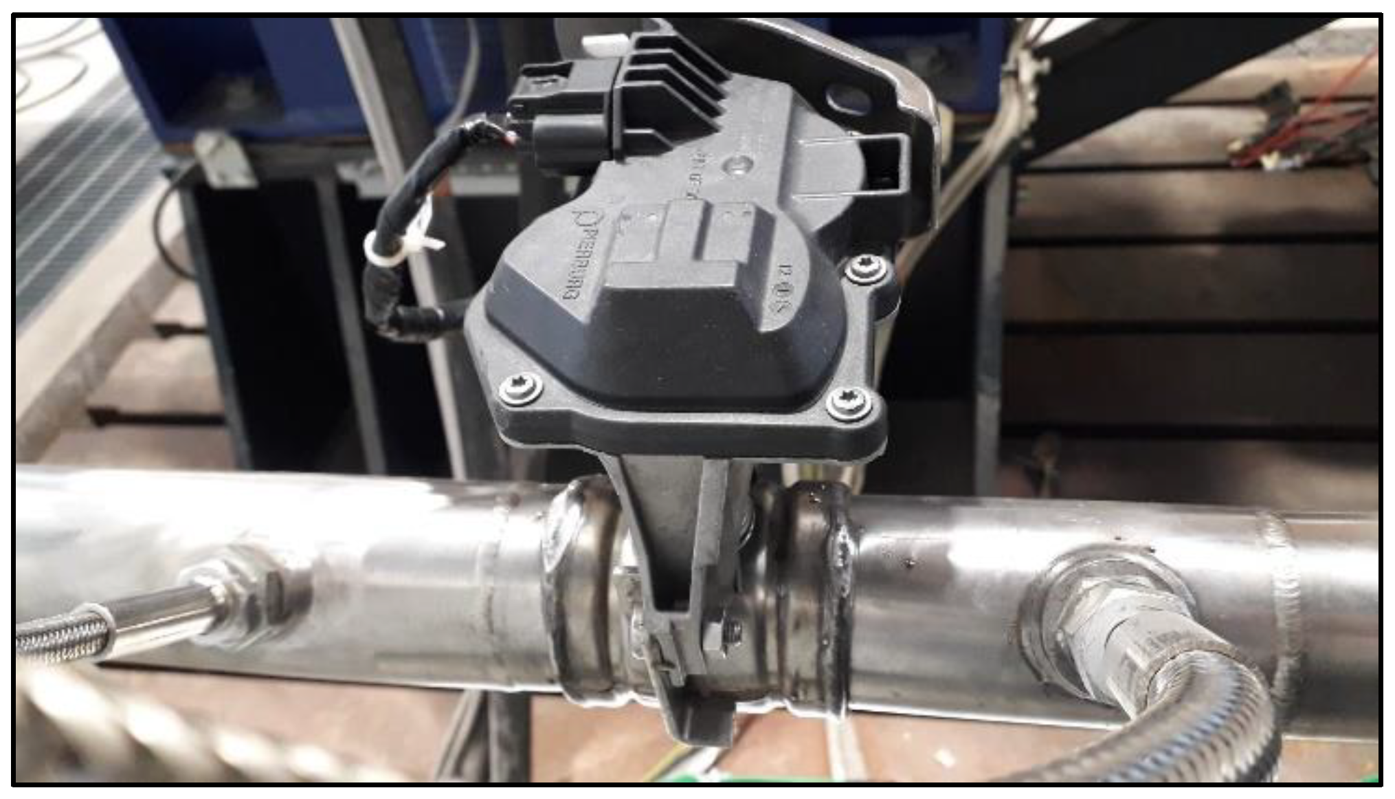
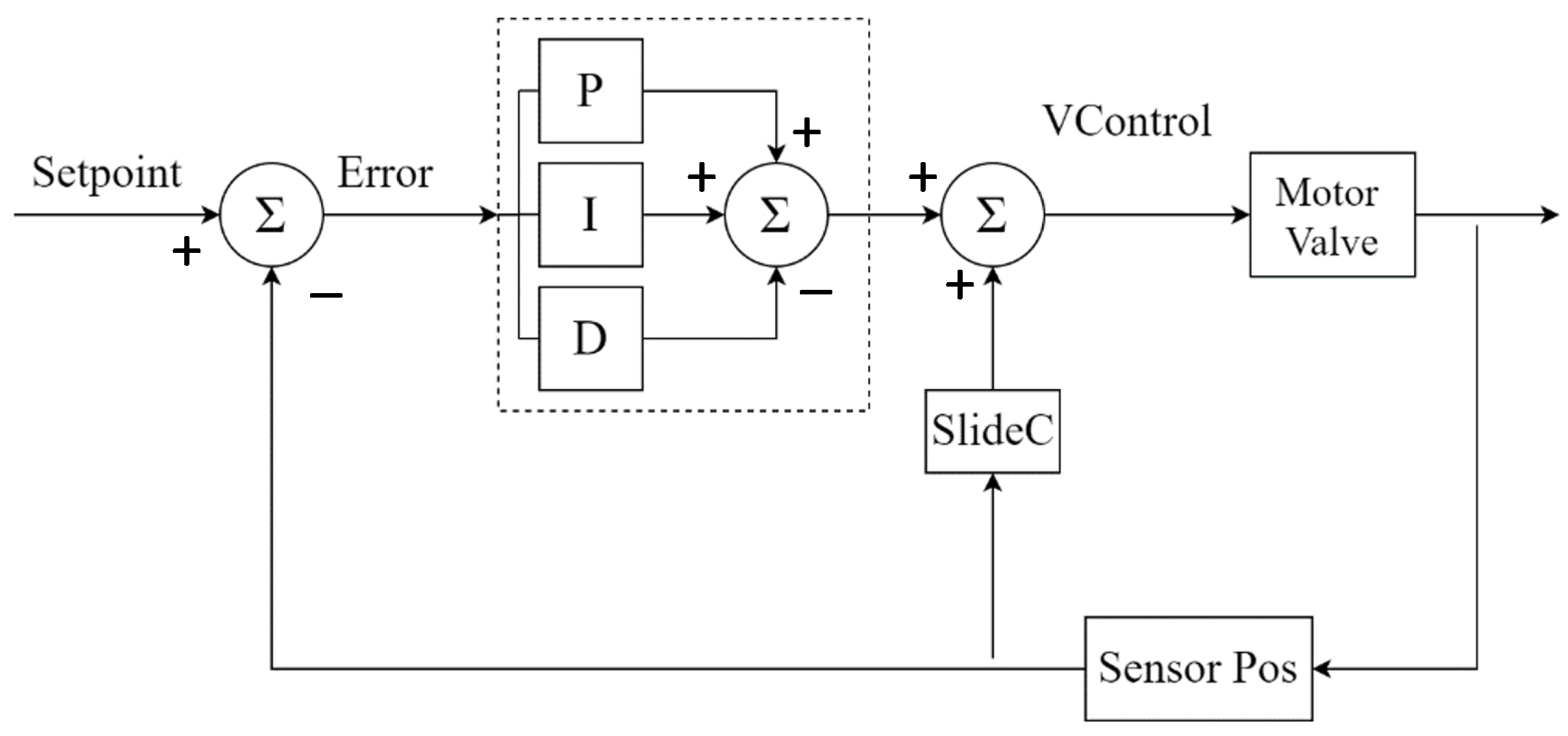
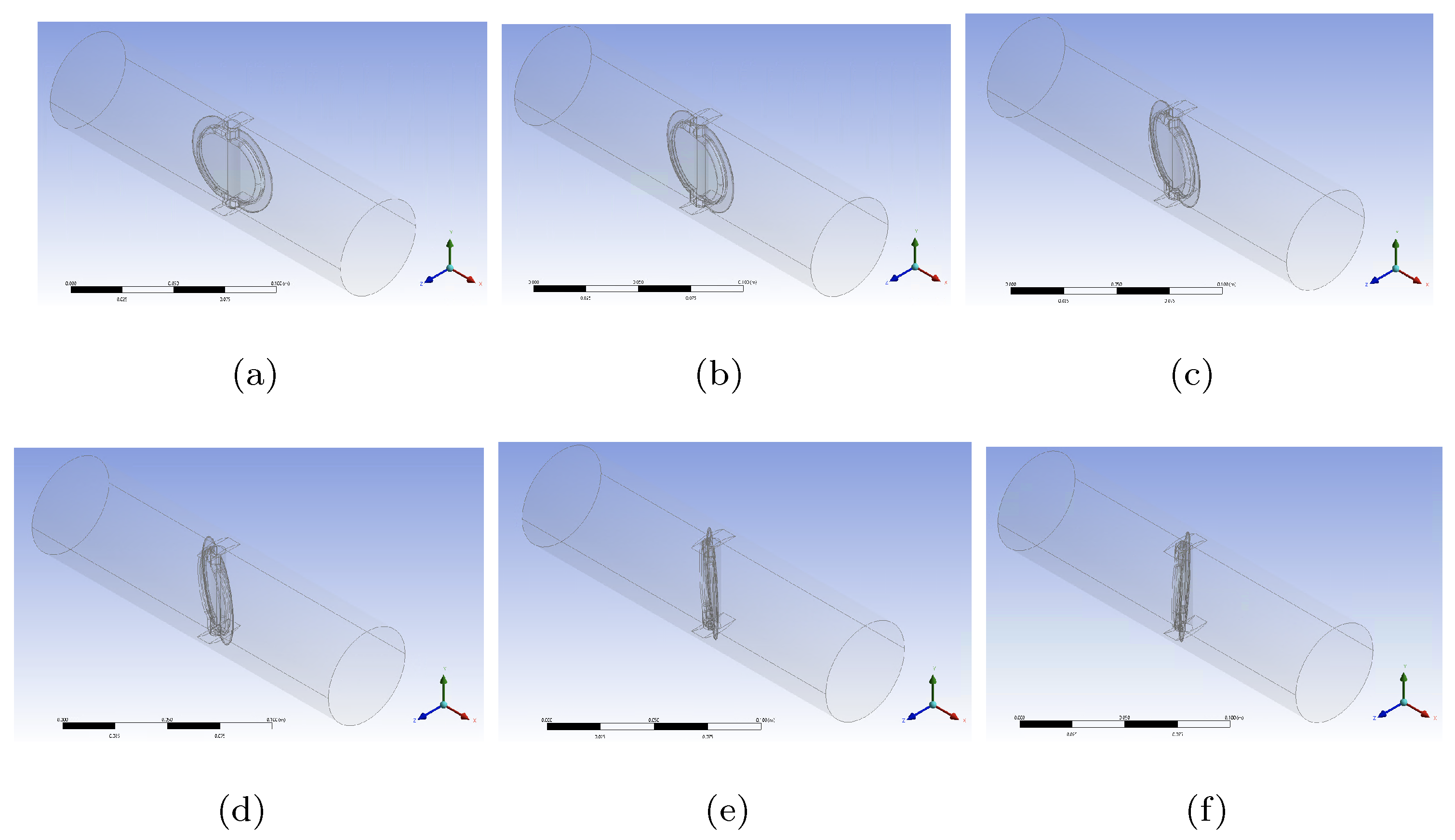
3.1. Back Pressure Valve

In Figure 5a,b, it is shown how the backpressure valve is not symmetrical. It is convex on the upstream flow side and concave on the downstream flow side. Additionally, it is not completely circular. The diameter of the valve at its central part is greater than the inner diameter of the pipe, so that when the valve is completely closed, touching the inside of the pipe, the angle between the plane of the valve and the axial axis of the pipe is approximately 70 degrees. The 3D model of the valve is shown in Figure 5c,d for the upstream flow side and downstream flow side, respectively.

Six models were created, one for each valve opening angle. As shown in Figure 6, the simulated valve openings range from 0 to 50 degrees in increments of 10 degrees. Figure 6 shows the isometric view of the six developed models.

The meshing of any of the models in Figure 6 was carried out taking into account the interaction of the fluid with the walls of the pipe and the valve using both hydrodynamic and thermal boundary layers. The inflation technique was used so that the maximum $y^{+}$ throughout the domain is less than 5, as shown in Figure 7. In this way, the shear stresses due to viscosity within the boundary layer are as close to reality as possible [11]. Four-node linear tetrahedrons and six-node linear wedges were used in the meshing. A mesh convergence study determined that the number of three-dimensional elements in the resulting mesh was between 3,400,000 and 4,000,000, depending on the valve opening. The quality of the mesh measured by the orthogonal quality parameter was around 0.15 in all cases, as a minimum value. As an example, Figure 7 shows the meshing of the model shown in Figure 6d.

It was considered that the radial temperature difference in the tube is negligible, and since the modelled valve is installed in a stationary engine test bench, heat dissipation outside the tube by natural convection, using the Churchill–Chu correlation, and radiation were considered. The inlet and outlet boundary conditions are of known mass flow rate and pressure, respectively. The turbulence boundary conditions are turbulent intensity equal to 5% and turbulent viscosity ratio equal to 10. The pressure–velocity coupling with the SIMPLE scheme was used as the solution method. Second-order spatial discretisation was used for pressure, density, momentum and energy, while first-order discretization was used for turbulent kinetic energy and turbulent dissipation rate. A convergence criterion of 10${}^{-3}$ was used for all variables, except for energy, which was set to 10${}^{-6}$.

For each valve opening angle, seven gas inlet temperatures to the valve were simulated, ranging from 200 to 500 °C in steps of 50 °C, and nine mass flow rates, ranging from 20 to 100 g/s in steps of 10 g/s. Therefore, a total of 6 × 7 × 9 = 378 simulations were carried out. The geometries were created in SolidWorks^®, the meshings were conducted in Ansys^® Meshing^® 2021 R2, and the simulations in Ansys^® Fluent^® 2021 R2.

The computer used to tune the models and perform sensitivity studies for each mesh was a Workstation Dell Precision 5820 with 28-core Intel Xeon W-2175, 2.5 GHz. The supercomputer used to perform the 378 simulations was Picasso, belonging to the University of Malaga, with 30,616 cores and 156 TB of RAM.

3.2. Turbulence Model

Mass flow rate was between 20 and 100 g/s. The average gas temperature was between 200 and 500 °C; thus, the dynamic viscosity was between 2.60 × 10${}^{-5}$ and 3.62 × 10${}^{-5}$ Pa·s.

Therefore, the average Reynolds number was between 13,500 and 94,200, indicating that the flow was predominantly turbulent. Turbulent flows can be simulated through computational fluid dynamic modelling using three different approaches: DNS (direct numerical simulation) [12], LES (large eddy simulation) [13,14], and RANS (Reynolds-averaged Navier–Stokes) [15]. The citation order corresponds to the decreasing calculation precision and increasing computational time cost.

As the bibliography review showed, most used methods for modelling the internal flow inside the exhaust pipe were Reynolds-averaged Navier–Stokes. Among the works which used the RANS method, most of the consulted works modelled the turbulence by means of $k-\epsilon$ equations [16,17,18,19]. This is justified by the reasonable balance between the computational time cost and the precision of the calculation method.

The present work is based on renormalisation group (RNG) $k-\epsilon$ turbulence modelling. This mathematical technique is used for solving the Navier–Stokes equations (Equations (1) and (2)) applied to each fluid. An exhaustive description of the RNG theory and its application to turbulent flows can be found in [20].

$$\frac{\partial }{\partial t}\left(\rho k\right)+\frac{\partial }{\partial x_i}\left(\rho k{u}_i\right)=\frac{\partial }{\partial x_j}\left({\alpha }_k{\mu }_{eff}\frac{\partial k}{\partial x_j}\right)+G_k+G_{bu}-\rho \epsilon -Y_M$$

(1)

$$\begin{array}{c}\hfill \frac{\partial }{\partial t}\left(\rho \epsilon \right)+\frac{\partial }{\partial x_i}\left(\rho \epsilon u_i\right)=\frac{\partial }{\partial x_j}\left({\alpha }_{\epsilon }{\mu }_{eff}\frac{\partial \epsilon }{\partial x_j}\right)+\\ \hfill C_{1\epsilon }\frac{\epsilon }{k}\left(G_k+C_{3\epsilon }{G}_{bu}\right)-C_{2\epsilon }\rho \frac{{\epsilon }^2}{k}-R_{\epsilon }\end{array}$$

(2)

In Equations (1) and (2), $G_k$ is the turbulence kinetic energy generation caused by the mean velocity gradients, $G_{bu}$ is the generation of turbulence kinetic energy due to the floatability, while $Y_M$ is the contribution of the dilatation variability in compressible turbulence to the overall dissipation rate. The terms ${\alpha }_k$ and ${\alpha }_{\epsilon }$ are the inverse of the Prandtl numbers for k and $\epsilon$, respectively.

For modelling thermal and hydrodynamic boundary layers, an enhanced wall treatment was used in Equation (2). Both pressure gradients and thermal effects were taken into account inside the boundary layers.

Enhanced wall treatment for the $\epsilon$-equation is a near-wall modelling method that combines a two-layer model with so-called enhanced wall functions. If the near-wall mesh is fine enough to be able to resolve the viscous sublayer (typically with the first near-wall node placed at $y^{+}\approx 1$), then the enhanced wall treatment will be identical to the traditional two-layer zonal model. However, the restriction that the near-wall mesh must be sufficiently fine everywhere might impose too large a computational requirement. Ideally, one would like to have a near-wall formulation that can be used with coarse meshes (usually referred to as wall-function meshes) as well as fine meshes (low-Reynolds number meshes). In addition, excessive error should not be incurred for the intermediate meshes where the first near-wall node is placed neither in the fully turbulent region, where the wall functions are suitable, nor in the direct vicinity of the wall, where the low-Reynolds number approach is adequate.

According to reference [21], the thermophysical properties of the exhaust gas are similar to those of air as a real gas at the same temperature and pressure. The majority of the composition of both gases is nitrogen. Both the density and viscosity of air vary with local pressure and temperature. The density of air was modelled using the Redlich–Kwong equation of state and dynamic viscosity using the Sutherland equation.

4. Results and Discussion

4.1. Test Results

4.1.1. Engine Operating Conditions

In

Table 1. Engine operating conditions.

Operating Mode:	A	B	C	D
Symbol in Figures	◯	△	□	♢
Engine speed (min${}^{-1}$)	1500	1500	2000	2500
Torque (Nm)	50	100	150	200
BMEP (bar)	3.98	8.07	11.77	16.50
$\dot{m}$ (g/s)	19.47	26.88	47.75	73.78
$T_{up}$ (°C)	241.12	309.83	353.46	432.42
$p_{up}$ (mbar)	3.38	6.15	22.50	52.81

, the measured average values for the four engine operating modes with the backpressure valve fully open are shown. $\dot{m}$ is the mass flow rate of exhaust gases. $T_{up}$ and $p_{up}$ are the temperature and pressure of the exhaust gases before the backpressure valve. As shown in Figure 8 and Figure 9, for each of the four engine operating modes, the backpressure valve was progressively closed in steps of 10% up to 50%, and from that point onwards, in steps of 5%. For operating mode A, the backpressure valve was closed up to 80%, for mode B up to 75%, for mode C up to 60%, and for mode D up to 50%. This sequence was chosen to avoid affecting the normal behaviour of the engine, so that the extra pressure drop caused by the valve closure was always less than 160 mbar.

4.1.2. Valve Closing

As shown in Figure 8, the mean instantaneous pressure inside the combustion chamber was experimentally measured for each engine operating mode and backpressure valve closure. A total of 1440 points per thermodynamic cycle of in-cylinder pressure were recorded (each pressure value was recorded every 0.5 degree of crank angle). For all operating modes, 20 thermodynamic cycles were recorded and used to calculate the mean in-cylinder pressure.

For all engine operating modes, except for the high-load mode (mode D), a slightly decreasing trend is observed between the measured instantaneous pressure inside the combustion chamber and the degree of closure of the backpressure valve, as shown in Figure 8a–c. This trend is consistent with that reported in [22]. This behaviour is consistent with the BMEP obtained for each mode (A, B, and C), as shown in Figure 9a. It can be concluded that, since the engine is turbocharged, a lower mass flow rate of exhaust gases through the turbine, as shown in Figure 9b, implies lower power production in the turbine and therefore lower power in the cylinder-boosting compressor, which slightly decreases the mean instantaneous pressure inside the combustion chamber.

From Figure 8d, no clear trend can be observed between the instantaneous mean pressure inside the cylinder and the closure of the back pressure valve for the high-load operating mode (Mode D). This may be because, regardless of the decrease in the mass flow rate of exhaust gases circulating through the turbine, as shown in Figure 9b, the energy of the exhaust gases is more than enough to power the turbine and, consequently, the compressor that supercharges the engine.

From Figure 9d, it can be observed that with the increase in the degree of closure of the backpressure valve and therefore the decrease in the mass flow rate, ash shown in Figure 9b, the average temperatures upstream of the backpressure valve increase. This may be due to the decrease in the circulation velocity of the exhaust gas, which leads to a lower convective heat transfer coefficient within the exhaust pipe and consequently to a lower rate of dissipation of heat power.

Figure 9c shows how the increase in the degree of closure of the back pressure valve leads to a potential increase in the pressure drop of the exhaust gas as it passes through the back pressure valve [7].

4.2. Model Results

As an example, Figure 10 shows the velocity, temperature, and pressure results in the axial plane, and Figure 11 shows the streamlines of a simulation with the valve rotated 30 degrees from fully open, a mass flow rate of 60 g/s, and an upstream exhaust gas temperature of 400 °C. The results obtained are consistent with [22]. It can be observed that the acceleration of the gas as it passes through the valve implies a significant decrease in temperature, as a result of the transfer of thermal energy to kinetic energy, and therefore an increase in pressure drop.

As discussed in Section 3.1, a total of 378 simulations were carried out, with the following combinations: mass flow rate equal to {20, 30, 40, 50, 60, 70, 80, 90, 100} (g/s), valve rotation angle with respect to the fully open position equal to {0, 10, 20, 30, 40, 50} degrees, and gas temperature upstream of the valve equal to {200, 250, 300, 350, 400, 450, 500} (°C). The results of all these simulations are represented in Figure 12, classified by the valve rotation angle.

In Figure 12, the colour map represents the drop in exhaust gas pressure in the valve under different conditions. Contour lines of constant exhaust gas pressure drop are shown. It can be observed that the valve angle and the exhaust gas mass flow rate are the two factors that most affect pressure drop, while the temperature of the exhaust gas has a less significant effect. An increase in the valve closure angle results in an increase in pressure drop [5], due to the increased flow velocity. An increase in the exhaust gas mass flow rate results in an increase in pressure drop, as the flow velocity increases and the pressure drop increases with higher flow rates. A slight increase in exhaust gas temperature results in a minor increase in pressure drop due to a decrease in density, resulting in a minor increase in gas velocity, while the mass flow rate remains constant.

In Figure 12, the experimental measurements of the four modes tested experimentally are shown. The percentage of valve closure in which the experimental pressure drop in the valve is of the same order as the pressure drop resulting from the modelling is shown in parentheses.

In experimental tests of flow in a back pressure valve, it is more cost-effective to measure the pressure drop using a differential pressure gauge than to measure the mass flow rate. Therefore, a correlation is proposed based on the results of the simulations that relate the four variables, Equation (3). The result of this correlation is the mass flow rate $\dot{m}$ in (g/s). A correlation coefficient of $R^2=0.984$ and a mean squared error of 0.32 were obtained.

$$\dot{m}=181.8{\left(1-sin\left(\theta \right)\right)}^{1.51}{T}^{-0.28}\Delta p^{0.50}$$

(3)

In Equation (3), $\theta$ is the angle of rotation of the valve with respect to the fully open position, T is the temperature of the gas upstream of the valve in °C, and $\Delta p$ is the pressure drop of the gas through the valve in mbar.

The experimental valve closing angle is difficult to measure, and even if it is measured, the actual value may differ from the assumed one. To quantify this deviation, the angle that the valve should have (y-axis of Figure 13) was compared with the experimental valve closing angle measured (x-axis of Figure 13).

In Figure 13, it is shown that there is a linear correlation between the experimentally measured valve closing angle and the valve angle obtained with the correlation of Equation (3). For all test modes with closing angles less than 50 degrees, there is a deviation of about 5 degrees between the two angles, with the experimentally measured angle being lower than the one obtained by the correlation.

5. Conclusions

The fluid-dynamic behaviour of an electronically controlled exhaust backpressure valve was analysed, operating at different opening degrees under different speed regimes and load degrees of a Euro 6 internal combustion engine. The following conclusions can be drawn from this research:

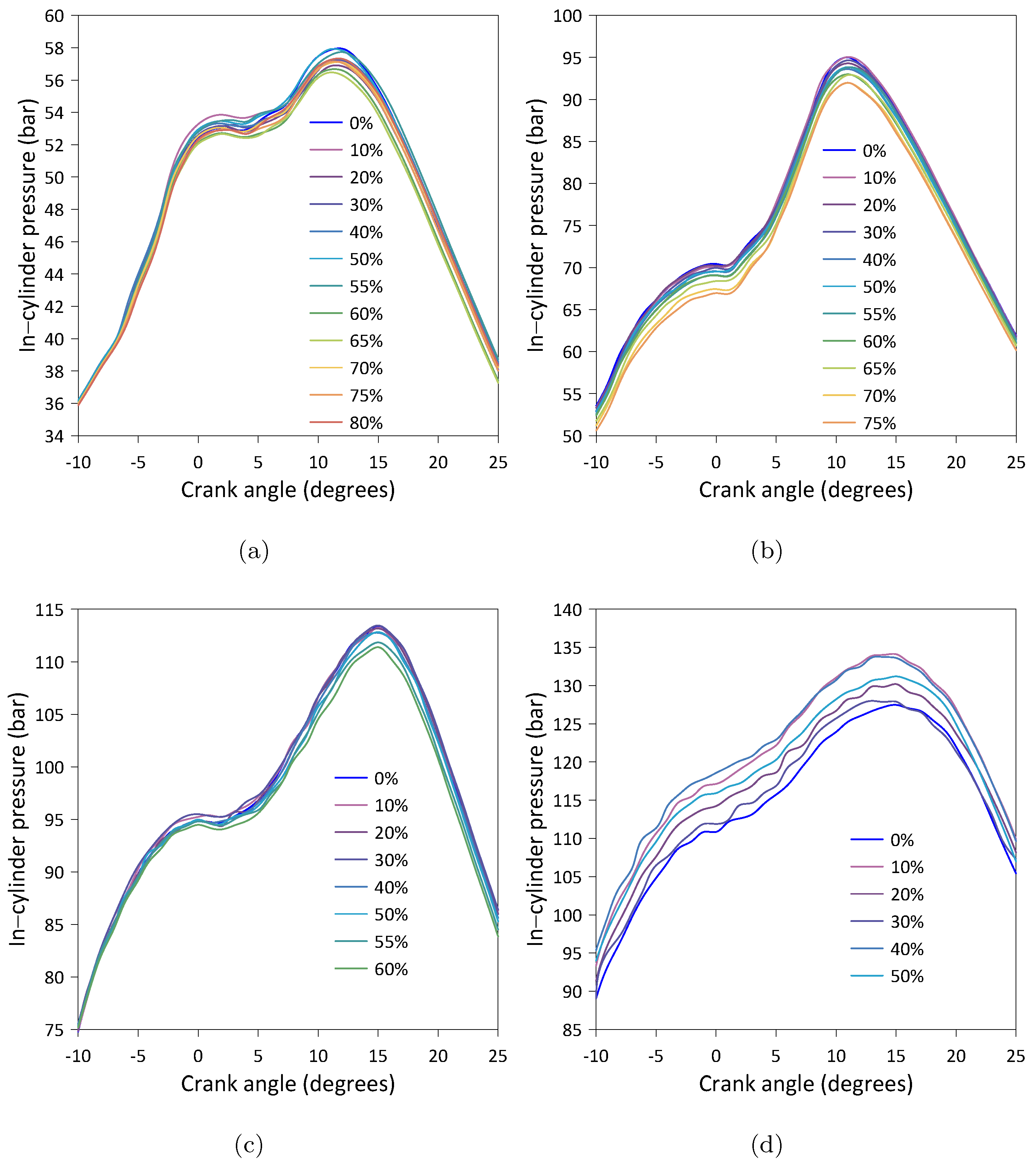
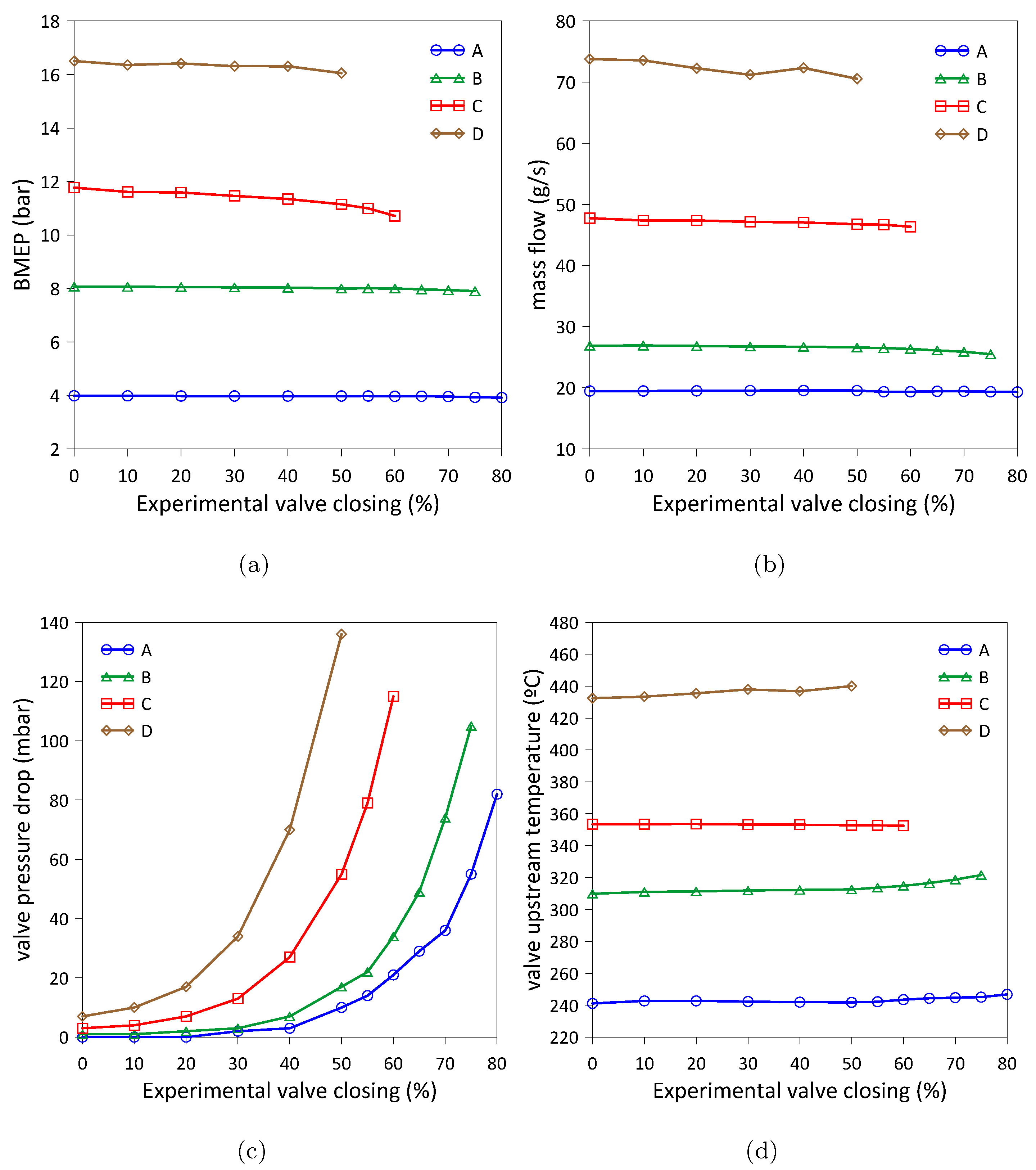
• The negative effect that the closure of the backpressure valve has on the instantaneous in-cylinder pressure was observed. Assuming no effect on the average pressure inside the cylinder with full opening, a reduction in the in-cylinder pressure was measured between 1.3% and 3.9% for valve closures between 50% and 80%, respectively, for medium–high load levels.
• It was observed that with an increase in the closure of the pressure relief valve, the effective average pressure of the engine decreases between 0.07 and 1.06 bar for valve closures between 50% and 80%, respectively, for medium–high load levels. However, for that range of valve closures, increases in the temperature of the exhaust gases upstream of the valve are observed between 5.7 and 11.7 °C.
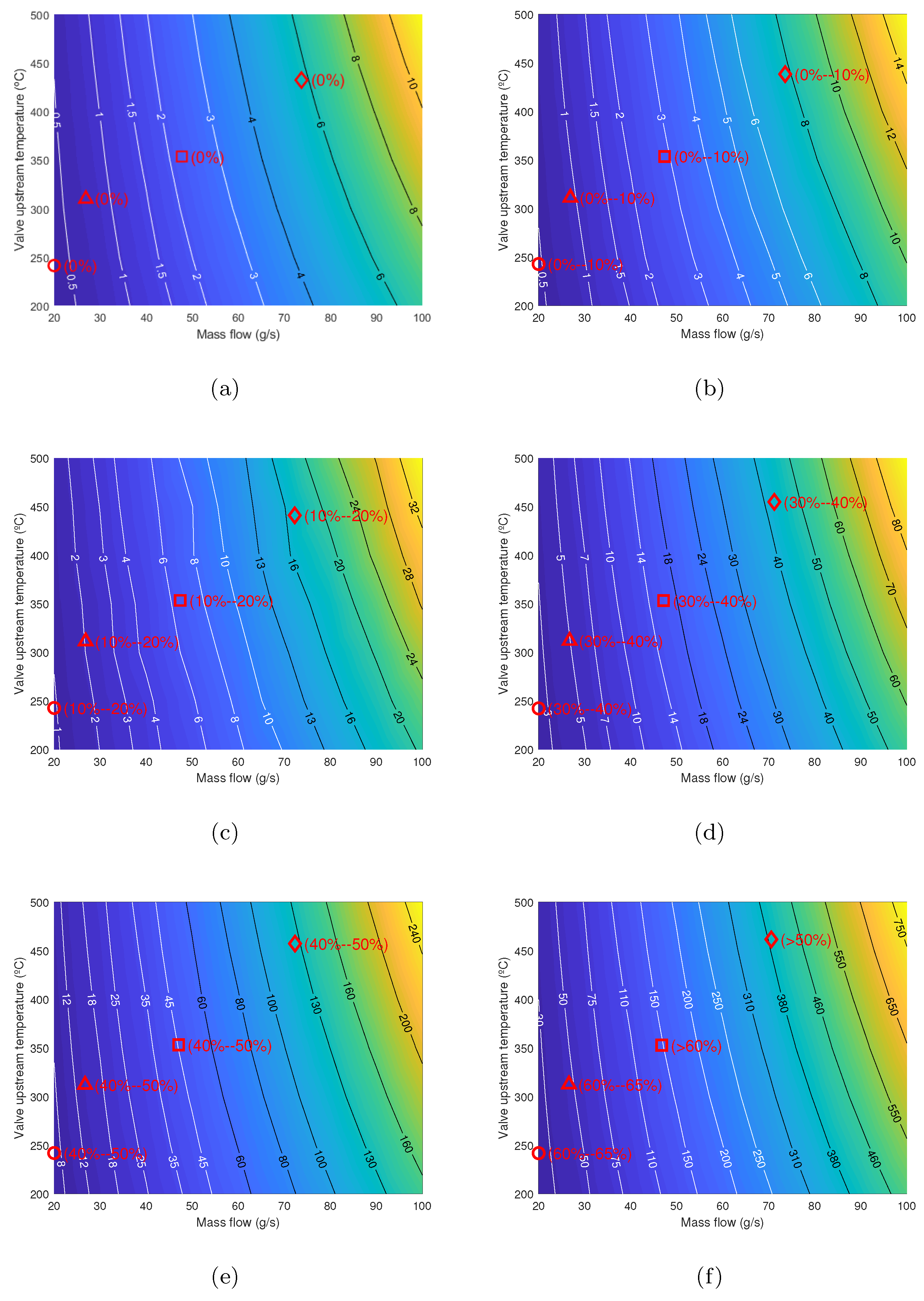
• The development of this work has made possible to propose a CFD model. With this model, the flow around the valve was simulated under different temperatures and the mass flows of exhaust gas and different closing positions of the backpressure valve. For all cases, pressure drop values were obtained. The level of agreement between the results obtained by the model compared to experimental measurements is around 91%.
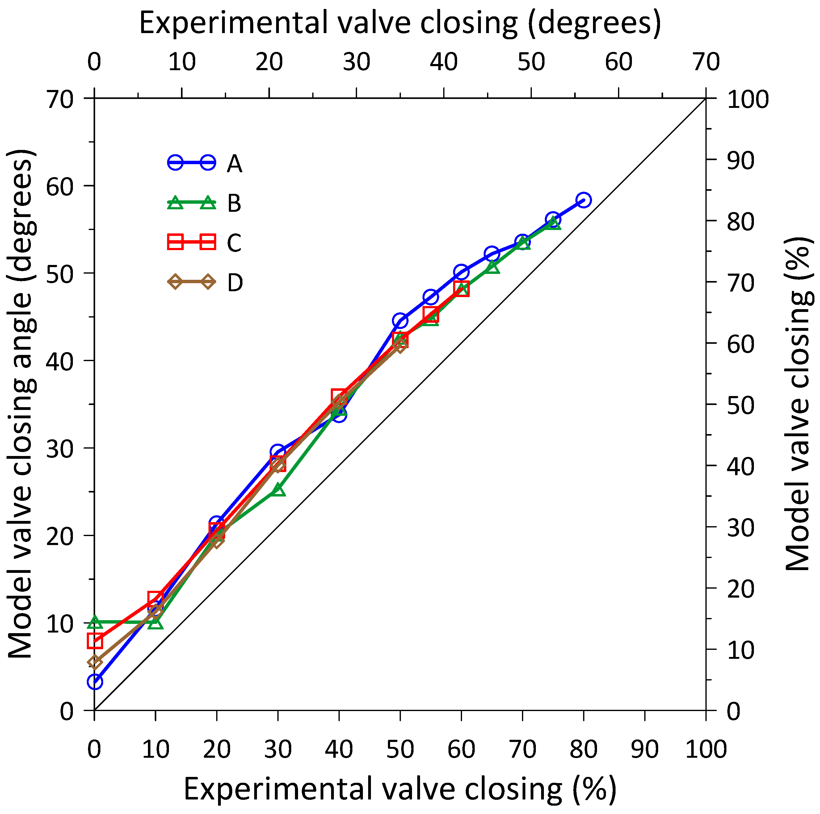
• The developed model helped to propose a correlation to estimate the mass flow rate of exhaust gas from easily measurable quantities on a test bench, such as gas temperature, valve closing angle, and pressure drop.
• A positive deviation of around 5 degrees of backpressure valve closing was obtained between the modelled angle and the experimental angle for all engine operating conditions and all valve closing angles.

References

1. Jovaj, M.S. Motores de Automóvil; Editorial MIR: Moscow, Russia, 1982. [Google Scholar]
2. Heywood, J.B. Internal Combustion Engine Fundamentals; McGraw-Hill Education: New York, NY, USA, 2018. [Google Scholar]
3. Payri González, F.; Desantes Fernández, J.M. Motores de Combustión Interna Alternativos; Editorial Universitat Politécnica de Valencia: Valencia, Spain, 2011. [Google Scholar]
4. Luján, J.M.; Guardiola, C.; Pla, B.; Reig, A. Switching strategy between HP (high pressure)-and LPEGR (low pressure exhaust gas recirculation) systems for reduced fuel consumption and emissions. Energy 2015, 90, 1790–1798. [Google Scholar] [CrossRef]
5. Choe, M.; Park, C.; Choi, D. Flow analysis on formation of back-pressure in exhaust system applying electronic-variable valve. Indian J. Sci. Technol. 2015, 8, 21. [Google Scholar] [CrossRef]
6. Pan, X.; Wang, G.; Lu, Z. Flow field simulation and a flow model of servo-valve spool valve orifice. Energy Convers. Manag. 2011, 52, 3249–3256. [Google Scholar] [CrossRef]
7. Long, C.; Guan, J. A method for determining valve coefficient and resistance coefficient for predicting gas flowrate. Exp. Therm. Fluid Sci. 2011, 35, 1162–1168. [Google Scholar] [CrossRef]
8. Gülmez, Y.; Özmen, G. Effect of exhaust backpressure on performance of a diesel engine: Neural network based sensitivity analysis. Int. J. Automot. Technol. 2022, 23, 215–223. [Google Scholar] [CrossRef]
9. Fernández-Yáñez, P.; Romero, V.; Armas, O.; Cerretti, G. Thermal management of thermoelectric generators for waste energy recovery. Appl. Therm. Eng. 2021, 196, 117291. [Google Scholar] [CrossRef]
10. Ezzitouni, S.; Fernández-Yáñez, P.; Sánchez, L.; Armas, O.; Soto, F. Effect of the use of a thermoelectric generator on the pumping work of a diesel engine. Int. J. Engine Res. 2021, 22, 1016–1027. [Google Scholar] [CrossRef]
11. Tuncer, C. Analysis of Turbulent Flows; Elsevier: Amsterdam, The Netherlands, 2004. [Google Scholar]
12. Reveillon, J.; Péra, C.; Bouali, Z. Examples of the potential of DNS for the understanding of reactive multiphase flows. Int. J. Spray Combust. Dyn. 2011, 3, 63–92. [Google Scholar] [CrossRef]
13. Piomelli, U. Large-eddy simulation: Achievements and challenges. Prog. Aerosp. Sci. 1999, 35, 335–362. [Google Scholar] [CrossRef]
14. De Villiers, E. The Potential of Large Eddy Simulation for the Modeling of Wall Bounded Flows; Imperial College of Science, Technology and Medicine: London, UK, 2006. [Google Scholar]
15. Versteeg, H.K.; Malalasekera, W. An Introduction to Computational Fluid Dynamics: The Finite Volume Method; Pearson Education: London, UK, 2007. [Google Scholar]
16. Kang, C.W.; Yi, C.S.; Jang, S.M.; Lee, C.W. A Study of the Measurement of the Flow Coefficient Cv of a Ball Valve for Instrumentation. J. Korean Soc. Manuf. Process. Eng. 2019, 18, 103–108. [Google Scholar] [CrossRef]
17. Laouar, S.; Sakib, M.N.; Al, S.M.; Navasardyan, M.V.; Kutsenko, K.V. Pressure drop in valve for different open flow areas. Proc. J. Phys. Conf. Ser. Iop Publ. 2020, 1439, 012009. [Google Scholar] [CrossRef]
18. Valdés, J.R.; Rodríguez, J.M.; Saumell, J.; Pütz, T. A methodology for the parametric modelling of the flow coefficients and flow rate in hydraulic valves. Energy Convers. Manag. 2014, 88, 598–611. [Google Scholar] [CrossRef]
19. Lisowski, E.; Filo, G. Analysis of a proportional control valve flow coefficient with the usage of a CFD method. Flow Meas. Instrum. 2017, 53, 269–278. [Google Scholar] [CrossRef]
20. Orszag, S.A.; Yakhot, V.; Flannery, W.S.; Boysan, F.; Choudhury, D.; Maruzewski, J.; Patel, B. Renormalization Group Modeling and Turbulence Simulations. In Proceedings of the International Conference on Near-Wall Turbulent Flows, Tempe, AZ, USA, 15–17 March 1993. [Google Scholar]
21. Lapuerta, M.; Armas, O.; Hernández, J. Diagnosis of DI Diesel combustion from in-cylinder pressure signal by estimation of mean thermodynamic properties of the gas. Appl. Therm. Eng. 1999, 19, 513–529. [Google Scholar] [CrossRef]
22. Ma, Z.; Zhang, K.; Xiang, H.; Gu, J.; Yang, M.; Deng, K. Experimental study on influence of high exhaust backpressure on diesel engine performance via energy and exergy analysis. Energy 2023, 263, 125788. [Google Scholar] [CrossRef]
Figure 1. (a) View of the instrumented engine exhaust system. (b) Front view of the engine test bench.
Energies 16 04112 g001
Figure 2. View of the exhaust back pressure valve.
Energies 16 04112 g002
Figure 3. Scheme of the connection of the control module.
Energies 16 04112 g003
Figure 4. Block diagram of the regulator used for the valve control.
Energies 16 04112 g004
Figure 5. Physical model of the valve: (a) upstream side of the valve, (b) downstream side of the valve, (c) upstream side 3D model, and (d) downstream side 3D model.
Energies 16 04112 g005
Figure 6. Three-dimensional model for each angle: (a) 0, (b) 10, (c) 20, (d) 30, (e) 40, and (f) 50 degrees.
Energies 16 04112 g006
Figure 7. Axial–vertical cross-section of a 3D meshed model of a valve rotated 30 degrees from fully open.
Energies 16 04112 g007
Figure 8. In-cylinder pressure vs. crank angle. (a) Mode A, (b) Mode B, (c) Mode C and (d) Mode D.
Energies 16 04112 g008
Figure 9. Average experimental data (a) BMEP, (b) mass flow, (c) valve pressure drop and (d) valve upstream temperature vs. valve closing.
Energies 16 04112 g009
Figure 10. Valve closing 30 degrees. Velocity (a), temperature (b) and pressure (c) field in axial plane.
Energies 16 04112 g010
Figure 11. Streamlines in the valve closing 30 degrees.
Energies 16 04112 g011
Figure 12. Pressure drop (mbar) vs. valve upstream temperature and mass flow. Closing angle: (a) 0, (b) 10, (c) 20, (d) 30, (e) 40 and (f) 50 degrees.
Energies 16 04112 g012
Figure 13. Model valve closing angle vs. experimental valve closing angle.
Energies 16 04112 g013