Non-Iterative, Unique, and Logical Formula-Based Technique to Determine Maximum Load Multiplier and Practical Load Multiplier for Both Transmission and Distribution Systems

Abstract

In recent days, due to the increasing number of electric vehicle charging stations (EVCSs) and additional power consumption by domestic, commercial, and industrial consumers, the overall power system performance suffers, which further degrades voltage profile, reduces stability, increases losses, and may also create a voltage collapse problem. Therefore, it is crucial to predetermine a maximum loadability limit for voltage collapse analysis and a practical allowable extra load for safe and secure operation, keeping the bus voltage within the security limits. To mitigate the problems, unique and innovative formulae such as the maximum load multiplier (MLM) and practical load multiplier (PLM) have been developed to consider line resistance. The determination of actual permissible extra load for a bus enables quick assessment of bus-wise suitable capacities and the number of EVs that can be charged simultaneously in the charging station. The planning engineers can easily settle on the extra load demand by domestic, commercial, and industrial consumers, while maintaining the voltage security constraint. The proposed technique is simple, non-iterative, computationally inexpensive, and applicable to both transmission and distribution systems. The proposed work is tested on a 57-bus transmission system and 69-bus radial distribution system, and the obtained results from the developed formulae are verified by comparing with conventional iterative methods.

1. Introduction

The use of air conditioners, induction heaters, washing machines, microwave ovens, mixers, computers, and laptops is rapidly expanding as individuals strive to lead a more luxurious lifestyle [1]. This surge in demand is not limited to domestic settings; industrial and commercial sectors are also experiencing a continuous increase in load demand. Consequently, it is essential to accurately assess power consumption to ensure the secure and stable operation of the power system [2]. Furthermore, the rise of electric vehicles (EVs) has revolutionized the transportation sector by reducing environmental pollution through the use of electricity instead of fossil fuels [3,4]. As the demand for EVs continues to soar, the number of charging stations connected to buses has also grown rapidly [5,6,7,8,9]. Consequently, there has been a sharp increase in power demand, which can potentially lead to voltage limit violations or voltage collapse. To mitigate these risks, two types of maximum additional loads for a bus are of utmost importance to determine. Using MLM, the maximum load margin or maximum loadability limit can be identified to avoid voltage collapse. Using PLM, the practical maximum allowable extra load for a bus can be evaluated for safe and secure power system operation, as the voltage should be within the security limits for practical operation.

To analyze voltage collapse and to know the load margin, the MLM is determined [10,11,12,13,14]. In this regard, the PV curve using Newton-Raphson Load Flow (NRLF) and continuation load flow (CLF) are commonly used [15,16,17,18,19,20,21]. In NRLF and CLF methods, both active and reactive loads are multiplied by the same multiplier to keep the power factor (pf) constant. Those methods are iterative methods and computationally expensive. Researchers and operating engineers of power systems also prefer simpler techniques and avoid programming complexity. In this context, the development of a non-iterative formula-based technique for the determination of maximum load limit would greatly assist in voltage stability analysis and enable easy identification of the voltage collapse point (VCP). To address this need, a unique and innovative formula has been devised for MLM calculation. This proposed technique is simple, non-iterative, and fast, offering a more efficient alternative. For verification of the results of the developed formula, voltage magnitude and execution time have been compared to well-known approaches, such as NRLF and CLF. In order to corroborate the formula, EVCSs are taken into consideration on load buses for both the 57-bus transmission system and the 69-bus radial distribution system (RDS), and the bus voltage result is evaluated to ensure that the security constraints are met.

From the voltage stability index (VSI), the weaker or weakest bus is identified [22,23,24,25,26]. Fast voltage stability index (FVSI) is commonly applied to find vulnerable buses as it takes less time [23,27,28]. It is also a non-iterative and formula-based technique. However, using FVSI, only the stability index or weaker buses can be determined, and MLM or load margin cannot be obtained. In addition, FVSI is not suitable for the distribution system as line resistance is neglected for calculation [29,30]. Thus, line resistance must be considered for developing MLM formulations to determine MLM or load margin. In [31], the authors have introduced a unique formula for calculating the maximum allowable active and reactive power for contingency analysis. In contrast, the proposed work involves calculating the maximum allowable load that can be added to a bus while ensuring system stability. In this regard, a new and effective formula for MLM determination is developed considering line resistance so that it can be applied in both transmission and distribution systems. Between these two formulae, one is considering the security constraints and other is not. In this paper, 57-bus as a transmission system [32,33] and 69-bus as RDS are [34,35] considered for result analysis.

Maximum loading capacity must be determined to avoid voltage instability or a voltage collapse problem. However, MLM cannot be used for practical power system operation since the voltage magnitude of the bus must be within security limitations in order to preserve power quality [36]. The allowable voltage range for the power system network is 0.9 to 1.1 p.u. [36,37]. Therefore, the practical allowable load which can be enhanced to a particular bus will be such that the voltage magnitude should not be less than 0.9 p.u. Considering the practical limits of voltage magnitudes of the buses, the PLM is formulated from MLM. Based on an extensive review of the existing literature, it is evident that a formula-based non-iterative PLM for both transmission and distribution systems was not developed at an early stage. However, this non-iterative approach is straightforward, efficient, and computationally inexpensive. By determining the PLM, it becomes possible to determine the maximum additional load that a bus can accommodate. For the different buses, different practical load margins will be attained. Hence, the most suitable capacity of an EV charging station can automatically be evaluated for the buses. Additionally, it enables the assessment of the number of EVs that can be charged simultaneously at the charging station. Furthermore, if the practical allowable extra load is known to the electricity company, it becomes feasible to promptly meet new load demands from residential, commercial, or industrial consumers in a justified and appropriate manner. The formulae of MLM and PLM are derived from the basic equation of line current, active power and reactive power flow, bus voltage, and phase angle of two buses of a single machine infinite bus (SMIB) system. The results obtained from PLM are also checked and verified with conventional methods such as CLF and NRLF.

The major contributions of this paper are as follows:

• A unique, innovative formula of MLM and PLM considering line resistance has been developed to evaluate the maximum load margin for voltage collapse and practical additional load for safe and secure power system operation, respectively, and the proposed formulae are applicable for both transmission and distribution systems.
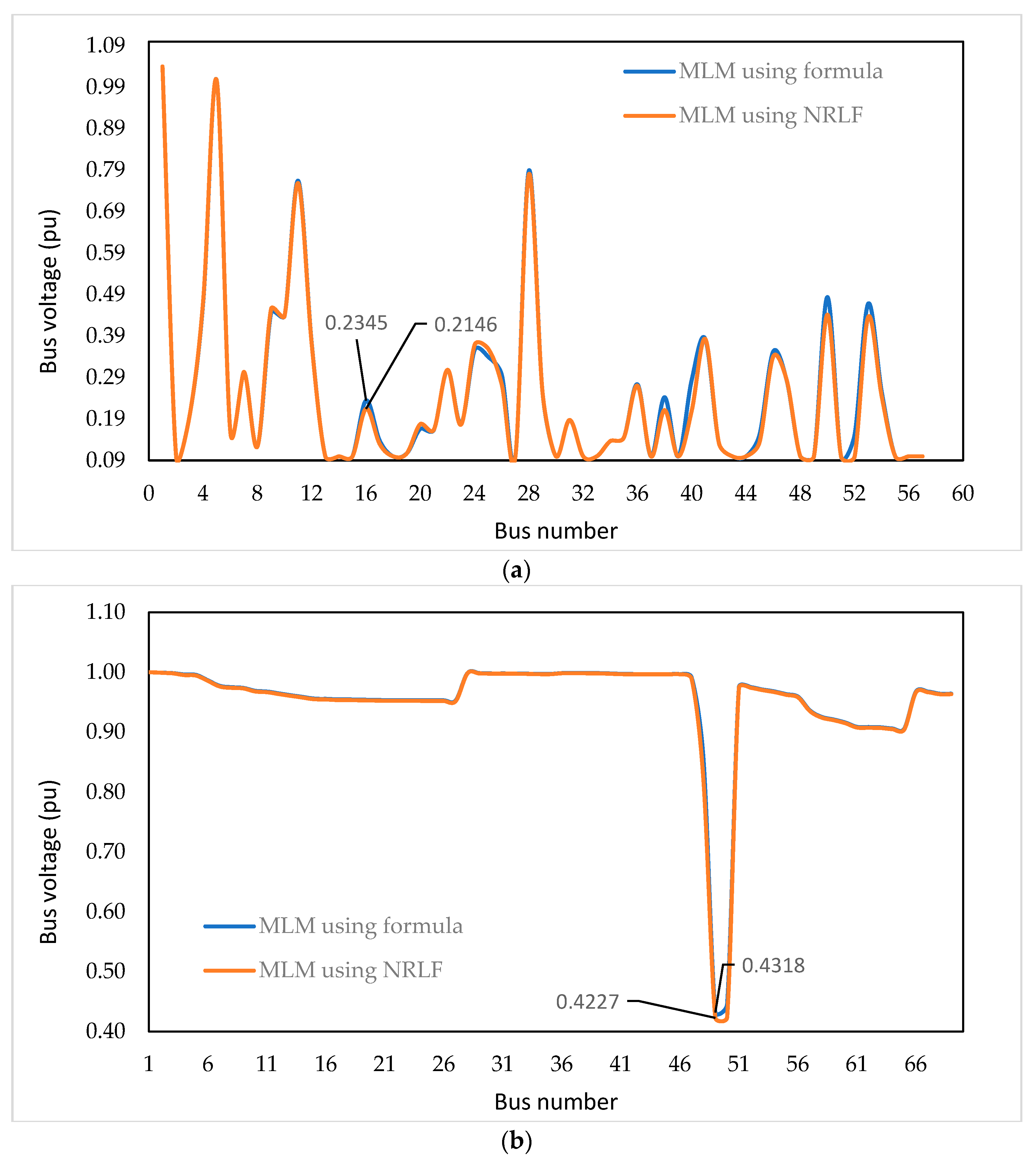
• The proposed technique is simple, non-iterative, and computationally inexpensive, and the obtained results from the developed formulae are vindicated by conventional iterative methods such as NRLF and CLF.
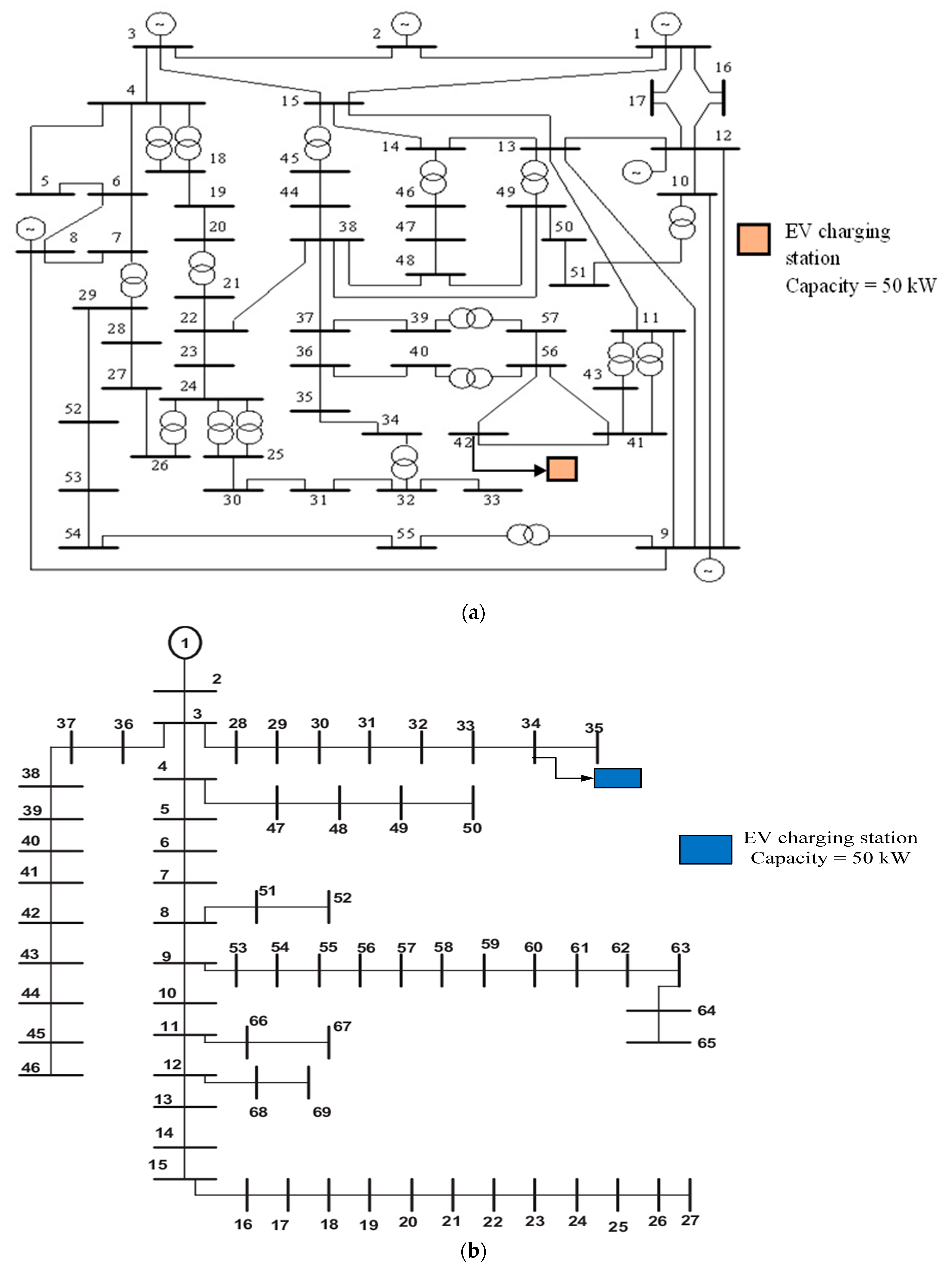
• As the actual permissible extra load for a bus is determined using PLM, the bus-wise suitable capacities or ratings of EV charging stations can quickly be assessed. The planning engineers can also easily settle on the extra load demand by the domestic, commercial, and industrial consumers, keeping the voltage magnitude within the security limit.

2. Problem Formulation

A fast and non-iterative technique to determine MLM and PLM is important in the present power scenario. New and innovative formulations are developed to determine MLM and PLM, which are computationally inexpensive as well as non-iterative. It is also applicable to both transmission and distribution systems. To derive the formula, a simple two-bus system of the SMIB system is considered. In Figure 1, a two-bus simple network is shown, where line resistance is not neglected. Here, Bus-1 represents the generator bus and Bus-2 represents the load bus. The formula of MLM and PLM is derived from the fundamental equations between the two buses, such as active power and reactive power flow, the current flowing between the two buses, bus voltages, phase angle, etc.

Where:

$V_1:$ A magnitude of the actual voltage at the sending end bus (SEB)

$V_2:$ A magnitude of the actual voltage at the receiving end bus (REB)

${\delta }_1:$ A phase angle of the voltage at the SEB

${\delta }_2:$ A phase angle of the voltage at the REB

$P_1:$ Active power at the SEB

$P_2:$ Active power at the REB

$Q_1:$ Reactive power at the SEB

$Q_2:$ Reactive power at the REB

Z: Line impedance between bus 1 and bus 2

$R_{12}:$ Line resistance between SEB and REB

$X_{12}:$ Line reactance between SEB and REB

$I_{12}:$ Line current between SEB and REB

Let,

$\delta ={\delta }_1-{\delta }_2:$ Phase angle difference between the SEB and REB

Considering both the resistance and reactance of the line, the MLM is formulated as

$$MLM=\frac{{\left|V_1\right|}^2}{2{\left(P_2{X}_{12}-Q_2{R}_{12}\right)}^2}\left\{\sqrt{\left[{\left(P_2{R}_{12}+Q_2{X}_{12}\right)}^2+{\left(P_2{X}_{12}-Q_2{R}_{12}\right)}^2\right]}-\left(P_2{R}_{12}+Q_2{X}_{12}\right)\right\}$$

(1)

The detailed derivation is given in Appendix A.

Equation (1) is the general formula of MLM, and it is useful for voltage collapse or voltage instability analysis. From MLM, for the practical operation of a power system, the maximum permissible load that can be applied practically to a bus cannot be obtained. The maximum allowable load for which the bus voltage will not violate the voltage limits is essential to determine safe and secure operation. The voltage of REB should be in the range of 0.9 p.u. to 1.1 p.u. [36,37]. However, by using (1), the bus voltage can decrease below 0.9 p.u., which is not acceptable for practical power system operation. Therefore, considering the practical limitations, the receiving end voltage should remain at 0.9 p.u. after the maximum allowable load enhancement. The generator bus voltage or SEB voltage is kept fixed. Considering the practical constraints, PLM is determined as follows:

$$\begin{array}{ll}PLM=& \frac{\sqrt{\left[\left\{4 \ast {\left(0.9\right)}^4 \ast {\left(P_2{R}_{12}+Q_2{X}_{12}\right)}^2\right\}-4 \ast \left\{{\left(P_2{R}_{12}+Q_2{X}_{12}\right)}^2+{\left(P_2{X}_{12}-Q_2{R}_{12}\right)}^2\right\} \ast \left\{{\left(0.9\right)}^4-{\left|V_1\right|}^2 \ast {\left(0.9\right)}^2\right\}\right]}}{2 \ast \left\{{\left(P_2{R}_{12}+Q_2{X}_{12}\right)}^2+{\left(P_2{X}_{12}-Q_2{R}_{12}\right)}^2\right\}}\\ & -\frac{{\left(0.9\right)}^2 \ast 2\left(P_2{R}_{12}+Q_2{X}_{12}\right)}{2 \ast \left\{{\left(P_2{R}_{12}+Q_2{X}_{12}\right)}^2+{\left(P_2{X}_{12}-Q_2{R}_{12}\right)}^2\right\}}\end{array}$$

(2)

From PLM, for the REB the actual additional load or practical load margin that can be enhanced while keeping the voltage magnitude in the security limits is obtained easily. It will be very helpful for the planning engineers to take a firm decision on the new load demand by the domestic/commercial/industrial consumers. Nowadays, EV charging stations are being installed worldwide. If the practical load margin is known for all buses, a suitable location and appropriate capacity of an EV charging station can also be determined.

3. Procedure

The formula used to calculate the MLM is employed in power systems to ensure the stability of the system. This formula is derived from (1). In this context, the bus at which MLM is calculated is referred to as the REB, while the bus supplying power to the REB is known as the SEB. The evaluation involves analysing two types of test systems: transmission and distribution systems. For the transmission system, 57-bus, and for RDS, 69-bus, are considered. As NRLF and CLF are commonly employed to determine MLM, the results of the unique and logical formula are compared to the results of the NRLF and CLF approaches. The load at the REB is gradually increased in conventional techniques, and convergence is tested in each run. When divergence occurs, MLM is determined for the conventional iterative methods and compared with the proposed technique.

For the practical operation of the power system, PLM is required instead of MLM so that the bus voltage will remain within the acceptable limit, 0.9 p.u. From MLM, PLM is derived, keeping the sending end voltage unaltered, and it is calculated using (2). The load multiplier for which the REB or the load bus voltage is at 0.9 p.u. is called PLM. Following the calculation of the PLM value using the proposed formula, the REB load will be multiplied by the PLM for both the NRLF and CLF techniques, and the results will be checked. The voltage magnitude should also be equal to 0.9 p.u. for the conventional methods. Being iterative methods, both NRLF and CLF take more time to give the desired results, whereas the proposed unique method gives the output directly as it is a non-iterative, formula-based approach.

After obtaining PLM for a specific bus, the extra load that can be allowed without violating the security constraints is analysed. As the maximum permissible additional load is established, the maximum acceptable new load demand or the suitable capacity of an EV charging station can be simply figured out. To carry out the load flow analysis, MATLAB-9.8 (R2020a) platform has been used. It was installed on a computer with an Intel i7 processor, 1.3 GHz clock speed and 8 GB RAM. A flow chart of the detailed procedure is given in Figure 2.

4. Result and Discussion

The developed formula of MLM and PLM is examined on both the interconnected transmission system, 57-bus, and RDS, 69-bus. The 57-bus system consists of 57 buses, 7 generators, 42 loads, and 63 transmission lines and has a base power of 100 MVA. The 69-bus system includes 69 buses and 73 lines and has a base voltage of 12.66 kV and a base power of 100 MVA.

For both the 57-bus transmission system and 69-bus RDS, 5 sets of buses are considered for finding MLM, PLM, and results analysis. The MLM of a bus is directly determined using (1) as the proposed approach is non-iterative and formula based. The MLM value is then reviewed by comparing it to the NRLF and CLF techniques. Comparison among NRLF, CLF, and the developed formula for MLM is shown in

Table 1. (a) Comparison among NRLF, CLF, and the developed formula for MLM for 57-Bus Transmission System. (b) Comparison among NRLF, CLF, and the developed formula for MLM for 69-Bus RDS.

(a)
Sl. No.	SEB	REB	MLM using formula	MLM using the NRLF method	MLM using the CLF method
1	12	16	14.1780	14.2968	14.2969
2	19	20	19.7453	19.2339	19.7465
3	13	14	55.1172	56.9040	56.9041
4	41	42	8.0156	7.6986	8.0156
5	50	51	15.1357	16.2367	16.2369
(b)
Sl. No.	SEB	REB	MLM using formula	MLM using the NRLF method	MLM using the CLF method
1	6	7	1850.9783	1851.1520	1851.1524
2	9	10	1254.8078	1254.8783	1254.8784
3	33	34	999.0980	998.9886	999.0981
4	48	49	123.3389	124.0974	124.8974
5	49	50	424.4114	423.8986	424.4114

a,b for both 57-bus transmission systems and 69-bus RDS, respectively. From Table 1a,b, it can be observed that the value of MLM calculated using (1) is nearly the same as the value of MLM obtained from the NRLF and CLF methods. Though MLM provides the maximum loading limits or VCPs, it is crucial to refrain from operating the power system at such loads due to the significantly lower voltage magnitude, which falls below the lower voltage limit of the network. Hence, PLM is of utmost importance in knowing the practical loading limit for safe, secure power system operation.

Being a non-iterative method, the proposed formulae take significantly less time to give the results as compared to iterative methods. To prove the efficacy of the proposed method, a comparison of estimation of MLM for both 57-bus and 69-bus systems is performed using the MATLAB platform. For the NRLF method, the load is gradually incremented and the estimation time is calculated. The estimation time is computed in seconds (s). The comparison of estimation time between proposed and conventional methods is shown in

Table 2. (a) Comparison of estimation time of MLM between the proposed method and the conventional method for a 57-bus transmission system. (b) Comparison of estimation time of MLM between the proposed method and the conventional method for a 69-bus RDS.

(a)
Sl. No.	SEB	REB	Estimation time for proposed method (s)	Estimation time for conventional method (NRLF) (s)
1	12	16	0.000901	3.976398
2	19	20	0.000468	13.11175
3	13	14	0.001183	25.28018
4	41	42	0.000526	3.034557
5	50	51	0.000591	6.391836
(b)
Sl. No.	SEB	REB	Estimation time for proposed method (s)	Estimation time for conventional method (NRLF) (s)
1	6	7	0.000581	683.3324
2	9	10	0.000594	493.4006
3	33	34	0.000432	410.1328
4	48	49	0.000498	36.969733
5	49	50	0.000414	176.776818

a,b for both 57- and 69-bus systems, respectively. From Table 2a,b, it is observed that the computation time is significantly less in the case of the proposed method as compared to the conventional method, which proves the effectiveness of the proposed work.

Like MLM, the PLM is directly determined using (2) for 5 sets of buses of 57-bus and 69-bus test systems. The obtained PLM value is used in conventional iterative methods such as CLF and NRLF. When PLM is applied to the REB, the voltage magnitude of REB should also be 0.9 p.u. for the conventional methods. In the case of conventional methods, the PLM is multiplied by the REB and the results are verified. The PLM obtained from the developed formula, and the voltage magnitude of REB for the conventional methods, are given in

Table 3. (a) Five sets of results of PLM for the 57-bus transmission system. (b) Five sets of results of PLM for 69-bus RDS.

(a)
Sl. No.	SEB.	REB	PLM obtained from developed formula	Receiving end voltage (p.u.)
1	12	16	6.99498	0.9031
2	19	20	5.74715	0.9082
3	13	14	18.49972	0.9015
4	41	42	2.99778	0.8981
5	50	51	8.02092	0.8994
(b)
Sl. No.	SEB.	REB	PLM obtained from developed formula	Receiving end voltage (p.u.)
1	6	7	616.4928	0.8997
2	9	10	372.218	0.8943
3	33	34	358.0564	0.9010
4	48	49	46.2458	0.8992
5	49	50	156.8488	0.9059

a,b for 57-bus and 69-bus systems, respectively. From the tables, it is observed that the voltage magnitude of the REB is nearly 0.9 p.u. It confirms that the PLM value obtained from the developed formula and it can be used for the safe and secure operation of the power system.

A graphical plot of voltage magnitude after applying PLM is shown below for both the 57- and 69-bus systems. After applying PLM at the 14th bus (REB), the voltage magnitude of the 57-bus transmission system is shown in Figure 3a. Similarly, the voltage magnitudes of a 69-bus RDS are given in Figure 3b when PLM is applied at the 34th bus (REB). From the two figures, it can be seen that the bus voltages of REB in both 57-bus and 69-bus test systems are the lowest and near 0.9 p.u. (i.e., 0.9015 p.u. and 0.9010 p.u., respectively), which is acceptable for practical operation. It is also observed that the bus voltage satisfies the lower voltage limit of the power system network.

A comparison of voltage magnitude is performed after employing a load multiplier in both the proposed approach and the conventional method for both the 57-bus transmission system and the 69-bus RDS. The value of the load multiplier is calculated using the proposed method as well as using the NRLF method. The proposed load multiplier, obtained from both cases, is applied to the REB, and voltage is observed.

Table 4. (a) Comparison of voltage magnitude after applying PLM obtained from both the conventional and proposed method for a 57-bus system. (b) Comparison of voltage magnitude after applying PLM obtained from both the conventional and proposed method for a 69-bus system.

(a)
SEB	REB	Voltage at REB after applying PLM, obtained from formula	Voltage at REB after applying PLM, obtained using NRLF
12	16	0.9031	0.9000
19	20	0.9082	0.9001
13	14	0.9015	0.9001
41	42	0.8981	0.8999
50	51	0.8994	0.9002
(b)
SEB	REB	Voltage at REB after applying PLM, obtained from formula	Voltage at REB after applying PLM, obtained using NRLF
6	7	0.8997	0.9002
9	10	0.8943	0.8999
33	34	0.9010	0.9000
48	49	0.8992	0.9003
49	50	0.9059	0.9001

a,b show the comparison of bus voltage magnitude after applying PLM in REB for both the 57-bus transmission system and the 69-bus RDS, respectively. From both tables, it is observed that the deviation in voltage at REB is very negligible. A graphical comparison of bus voltage is also shown below. The 16th bus in the 57-bus transmission system serves as an illustrative example to demonstrate the comparison of voltage magnitude between the conventional and proposed method for both PLM and MLM cases. These comparisons are presented in Figure 4a and Figure 5a for the 57-bus system. Similarly, in the case of the 69-bus RDS, the 49th bus is selected as a sample example to showcase the voltage magnitude comparison between the conventional and proposed method for both PLM and MLM. Figure 4b and Figure 5b display these comparisons for the 69-bus RDS. From Figure 4a,b, it is observed that there is a slight deviation in the voltage magnitude at the bus where the PLM is implemented, though the deviation is trivial/insignificant. However, the voltage magnitudes at the remaining buses (i.e., all other buses) are similar/matching for both the proposed method and the conventional method. Both the figures depict that the result attained using the proposed method is matching with the result obtained from the conventional iterative method (NRLF).

Figure 5a,b show the comparison of bus voltage between conventional and proposed methods when MLM is applied at REB for both the 57-bus transmission system and the 69-bus RDS, respectively. MLM is generally calculated to identify the VCP. Therefore, the voltage security constraint is not maintained in the case of MLM. From both the figures, it is observed that the there is a slight variation in voltage, mostly where the MLM is applied in the proposed method as compared to the conventional method. On the other hand, voltage magnitude of the rest of the buses are almost the same in both the conventional and the proposed method. Therefore, it can be concluded that the proposed method for calculating the load multiplier gives the correct result.

The maximum additional load that can be added with the base load using MLM is given in

Table 5. (a) Maximum extra load that can be added with base load using MLM for a 57-bus system. (b) Maximum extra load that can be added with base load using MLM for a 69-bus system.

(a)
Sl. No.	SEB.	REB	Base load at RE		Modified load after multiplying MLM at RE		Additional load at RE
			${\mathit{P}}_{\mathit{L}}$ (MW)	${\mathit{Q}}_{\mathit{L}}$  (MVAr)	${\mathit{P}}_{\mathit{L}}$ (MW)	${\mathit{Q}}_{\mathit{L}}$ (MVAr)	${\mathit{P}}_{\mathit{L}}$ (MW)	${\mathit{Q}}_{\mathit{L}}$ (MVAr)
1	12	16	43	3	678.5787	47.3427	635.5787	44.3427
2	19	20	2.3	1	45.4142	19.7453	43.1142	18.7453
3	13	14	10.5	5.3	578.7306	292.1212	568.2306	286.8212
4	41	42	7.1	4	56.9113	32.0627	49.8113	28.0627
5	50	51	18	5.3	218.4341	64.3167	200.4341	59.0167
(b)
Sl. No.	SEB	REB	Base load at RE		Modified load after multiplying MLM at RE		Additional load at RE
			${\mathit{P}}_{\mathit{L}}$ (MW)	${\mathit{Q}}_{\mathit{L}}$ (MVAr)	${\mathit{P}}_{\mathit{L}}$ (MW)	${\mathit{Q}}_{\mathit{L}}$ (MVAr)	${\mathit{P}}_{\mathit{L}}$ (MW)	${\mathit{Q}}_{\mathit{L}}$ (MVAr)
1	6	7	0.04	0.03	74.0332	55.5249	73.9932	55.4949
2	9	10	0.03	0.02	37.6202	25.0802	37.5902	37.6002
3	33	34	0.02	0.01	19.982	9.991	19.962	9.981
4	48	49	0.38	0.27	46.8688	33.3025	46.4888	33.0315
5	49	50	0.38	0.27	161.2763	114.5911	160.8963	114.3211

a,b for the 57-bus System and the 69-bus RDS, respectively. From the tables, the maximum extra load for which the system will be at the VCP can be assessed for voltage stability analysis. The maximum practical allowable load obtained from PLM is shown in

Table 6. (a) Maximum practical allowable load obtained from PLM for a 57-bus system. (b) Maximum practical allowable load obtained from PLM for a 69-bus RDS.

(a)
Sl. No.	SEB	REB	Base load at RE		Modified load after multiplying PLM at RE		Additional load at RE
			${\mathit{P}}_{\mathit{L}}$ (MW)	${\mathit{Q}}_{\mathit{L}}$ (MVAr)	${\mathit{P}}_{\mathit{L}}$ (MW)	${\mathit{Q}}_{\mathit{L}}$ (MVAr)	${\mathit{P}}_{\mathit{L}}$ (MW)	${\mathit{Q}}_{\mathit{L}}$ (MVAr)
1	12	16	43	3	300.7841	20.9849	257.7841	17.9849
2	19	20	2.3	1	13.2184	5.7471	10.9184	4.7471
3	13	14	10.5	5.3	194.2471	98.0485	183.7471	92.7485
4	41	42	7.1	4	21.2842	11.9911	14.1842	7.9911
5	50	51	18	5.3	144.3766	42.5109	126.3766	37.2109
(b)
Sl. No.	SEB	REB	Base load at RE		Modified load after multiplying PLM at RE		Additional load at RE
			${\mathit{P}}_{\mathit{L}}$ (MW)	${\mathit{Q}}_{\mathit{L}}$ (MVAr)	${\mathit{P}}_{\mathit{L}}$ (MW)	${\mathit{Q}}_{\mathit{L}}$ (MVAr)	${\mathit{P}}_{\mathit{L}}$ (MW)	${\mathit{Q}}_{\mathit{L}}$ (MVAr)
1	6	7	0.04	0.03	24.66	18.495	24.62	18.465
2	9	10	0.03	0.02	11.17	7.44	11.14	7.42
3	33	34	0.02	0.01	7.16	3.58	7.14	3.57
4	48	49	0.38	0.27	17.57	12.49	17.19	12.22
5	49	50	0.38	0.27	59.6	42.35	59.22	42.08

a,b for the 57-bus transmission system and the 69-bus RDS, respectively. The tables provide information on both active and reactive power loads that are permissible for ensuring safe and stable operation of the power system. From the tables, bus-wise practical permissible load enhancement is known, and it will be very useful for the permission of new connections and extra load demands by the existing consumers. In light of the recent installation of EV charging stations on buses, planning engineers can efficiently determine the most suitable buses and charging station capacities by referring to the acquired actual extra load data.

The proposed approach is rationalized by taking into account EVCS on load buses of the 57-bus transmission system and 69-bus RDS. The DC fast charging station with a capacity of 50 kW is considered to be placed on the load buses, and the bus voltage at the REB is shown in

Table 7. (a) Voltages at REB after placing charging station on load bus for a 57-bus transmission system. (b) Voltages at REB after placing charging station on load bus for a 69-bus RDS.

(a)
Sl. No.	SEB	REB	Base active power load at receiving end bus (MW)	Base reactive power load at receiving end bus (MVAr)	Voltage at receiving end bus (p.u.)
1	12	16	43	3	1.0134
2	19	20	2.3	1	0.9626
3	13	14	10.5	5.3	0.9681
4	41	42	7.1	4	0.9682
5	50	51	18	5.3	1.0520
(b)
Sl. No.	SEB	REB	Base active power load at receiving end bus (MW)	Base reactive power load at receiving end bus (MVAr)	Voltage at receiving end bus (p.u.)
1	6	7	0.04	0.03	0.9805
2	9	10	0.03	0.02	0.9718
3	33	34	0.02	0.01	0.9971
4	48	49	0.38	0.27	0.9944
5	49	50	0.38	0.27	0.9937

a,b for the 57-bus system and 69-bus RDS, respectively. From Table 7a,b it is observed that the voltage levels at the load bus remain within the prescribed security limits of 0.9 p.u. to 1.1 p.u. after the installation of the electric vehicle (EV) charging station. This outcome effectively fulfills the voltage constraints. Figure 6a shows a simplified figure of a 57-bus transmission system indicating the EV charging station at the 42nd load bus. Figure 6b represents a simplified figure of a 69-bus RDS indicating the EV charging station at the 34th load bus.

5. Conclusions

For finding the MLM and PLM, unique and innovative formulae considering line resistance are so developed that they can be applied for both the transmission and distribution systems. These formulae can be effectively applied to both transmission and distribution systems. This research paper focuses on the 57-bus test system for transmission and the 69-bus test system for distribution. MLM gives the VCP, or maximum loadability limit, which is useful for voltage stability analysis. On the other hand, it is essential to ensure the safe, reliable, and practical operation of the power system by maintaining the voltage magnitude above the lower limit of voltage constraints limit (i.e., 0.9–1.1 p.u.). In light of the idea, an efficient and logical formula for PLM is developed to calculate the maximum practical permitted load for a particular bus. To justify the results of the newly proposed simple formulae, a comparison is done between the results obtained from the NRLF and CLF methods and the result obtained from the proposed non-iterative formula-based techniques. To compare the simulation time, a comparison of estimated time is also performed to showcase the effectiveness of the proposed formula. From the results, it can be concluded that the developed formulae are very effective and fruitful for planning engineers to decide about new connections, additional load demand by the existing consumers, or the optimum capacity of an EV charging station for a bus, and also it takes less time as compared to the conventional method to get the result. The application of EV fast charging stations is also implemented for both 57-bus and 69-bus test systems to prove the efficacy of the proposed method.

References

1. Prudenzi, A.; Silvestri, A.; Lucci, G.; Regoli, M. Analysis of Residential Standby Power Demand Control through a Psychological Model of Demand. In Proceedings of the 10th International Conference on Environment and Electrical Engineering, Rome, Italy, 8–11 May 2011. [Google Scholar]
2. Tang, X.; Milanovic, J.V. Assessment of the Impact of Demand Side Management on Power System Small Signal Stability. In Proceedings of the IEEE Manchester Power Tech, Manchester, UK, 18–22 June 2017. [Google Scholar]
3. Tuscano, A.A.; Gabhane, S.K. A Method for Optimal Usage of Power in Electric Vehicle. In Proceedings of the International Conference on Inventive Computation Technologies (ICICT), Coimbatore, India, 26–27 August 2016. [Google Scholar]
4. Joshi, A.; Sharma, R.; Baral, B. Comparative Life Cycle Assessment of Conventional Combustion Engine Vehicle, Battery Electric Vehicle and Fuel Cell Electric Vehicle in Nepal. J. Clean. Prod. 2022, 379, 134407. [Google Scholar] [CrossRef]
5. Mastoi, M.S.; Zhuang, S.; Munir, H.M.; Haris, M.; Hassan, M.; Usman, M.; Bukhari, S.S.H.; Ro, J.-S. An In-Depth Analysis of Electric Vehicle Charging Station Infrastructure, Policy Implications, and Future Trends. Energy Rep. 2022, 8, 11504–11529. [Google Scholar] [CrossRef]
6. Nafi, I.M.; Tabassum, S.; Hassan, Q.R.; Abid, F. Effect of Electric Vehicle Fast Charging Station on Residential Distribution Network in Bangladesh. In Proceedings of the 5th International Conference on Electrical Engineering and Information Communication Technology (ICEEICT), Dhaka, Bangladesh, 18–20 November 2021. [Google Scholar]
7. Nutkani, I.U.; Lee, J.C. Evaluation of Electric Vehicles (EVs) Impact on Electric Grid. In Proceedings of the International Power Electronics Conference (IPEC-Himeji 2022-ECCE Asia), Himeji, Japan, 15–19 May 2022. [Google Scholar]
8. Savari, G.F.; Sathik, M.J.; Raman, L.A.; El-Shahat, A.; Hasanien, H.M.; Almakhles, D.; Abdel Aleem, S.H.E.; Omar, A.I. Assessment of Charging Technologies, Infrastructure and Charging Station Recommendation Schemes of Electric Vehicles: A Review. Ain Shams Eng. J. 2023, 14, 101938. [Google Scholar] [CrossRef]
9. Olcay, K.; Çetinkaya, N. Analysis of the Electric Vehicle Charging Stations Effects on the Electricity Network with Artificial Neural Network. Energies 2023, 16, 1282. [Google Scholar] [CrossRef]
10. Adebayo, I.G.; Sun, Y. Performance Evaluation of Voltage Stability Indices for a Static Voltage Collapse Prediction. In Proceedings of the IEEE PES/IAS PowerAfrica, Nairobi, Kenya, 25–28 August 2020. [Google Scholar]
11. Bento, M.E.C. A Method for Monitoring the Load Margin of Power Systems under Load Growth Variations. Sustain. Energy Grids Netw. 2022, 30, 100677. [Google Scholar] [CrossRef]
12. Adetokun, B.B.; Muriithi, C.M.; Ojo, J.O. Voltage Stability Assessment and Enhancement of Power Grid with Increasing Wind Energy Penetration. Int. J. Electr. Power Energy Syst. 2020, 120, 105988. [Google Scholar] [CrossRef]
13. Mallick, S.; Acharjee, P.; Ghoshal, S.P.; Thakur, S.S. Determination of Maximum Load Margin Using Fuzzy Logic. Int. J. Electr. Power Energy Syst. 2013, 52, 231–246. [Google Scholar] [CrossRef]
14. Bonini Neto, A.; Alves, D.A.; Minussi, C.R. Artificial Neural Networks: Multilayer Perceptron and Radial Basis to Obtain Post-Contingency Loading Margin in Electrical Power Systems. Energies 2022, 15, 7939. [Google Scholar] [CrossRef]
15. Mishra, S.; Brar, Y.S. Load Flow Analysis Using MATLAB. In Proceedings of the IEEE International Students’ Conference on Electrical, Electronics and Computer Science (SCEECS), Bhopal, India, 19–20 February 2022. [Google Scholar]
16. Chatterjee, S.; Mandal, S. A Novel Comparison of Gauss-Seidel and Newton- Raphson Methods for Load Flow Analysis. In Proceedings of the International Conference on Power and Embedded Drive Control (ICPEDC), Chennai, India, 16–18 March 2017. [Google Scholar]
17. Ajjarapu, V.; Christy, C. The Continuation Power Flow: A Tool for Steady State Voltage Stability Analysis. IEEE Trans. Power Syst. 1992, 7, 416–423. [Google Scholar] [CrossRef]
18. Lou, Y.; Ou, Z.; Tong, Z.; Tang, W.; Li, Z.; Yang, K. Static Volatge Stability Evaluation on the Urban Power System by Continuation Power Flow. In Proceedings of the 5th International Conference on Energy, Electrical and Power Engineering (CEEPE), Chongqing, China, 22–24 April 2022. [Google Scholar]
19. Jmii, H.; Meddeb, A.; Chebbi, S. Newton-Raphson Load Flow Method for Voltage Contingency Ranking. In Proceedings of the 15th International Multi-Conference on Systems, Signals & Devices (SSD), Hammamet, Tunisia, 19–22 March 2018. [Google Scholar]
20. Thiyagarajan, T.; Mv, S.; Samy, A.K.; Venkadesan, A. Performance Investigation of SVR for Evaluating Voltage Stability Margin in a Power Utility. In Proceedings of the IEEE International Power and Renewable Energy Conference (IPRECON), Kollam, India, 24–26 September 2021. [Google Scholar]
21. Montoya, O.D.; Gil-Gonzalez, W.; Garrido, V.M. Voltage Stability Margin in DC Grids with CPLs: A Recursive Newton–Raphson Approximation. IEEE Trans. Circuits Syst. II 2020, 67, 300–304. [Google Scholar] [CrossRef]
22. Roy Ghatak, S.; Sannigrahi, S.; Acharjee, P. Comparative Performance Analysis of DG and DSTATCOM Using Improved PSO Based on Success Rate for Deregulated Environment. IEEE Syst. J. 2018, 12, 2791–2802. [Google Scholar] [CrossRef]
23. Modarresi, J.; Gholipour, E.; Khodabakhshian, A. A Comprehensive Review of the Voltage Stability Indices. Renew. Sustain. Energy Rev. 2016, 63, 1–12. [Google Scholar] [CrossRef]
24. Mokred, S.; Wang, Y.; Chen, T. Modern Voltage Stability Index for Prediction of Voltage Collapse and Estimation of Maximum Load-Ability for Weak Buses and Critical Lines Identification. Int. J. Electr. Power Energy Syst. 2023, 145, 108596. [Google Scholar] [CrossRef]
25. Kayal, P.; Chanda, C.K. Placement of Wind and Solar Based DGs in Distribution System for Power Loss Minimization and Voltage Stability Improvement. Int. J. Electr. Power Energy Syst. 2013, 53, 795–809. [Google Scholar] [CrossRef]
26. Danish, M.S.S.; Senjyu, T.; Danish, S.M.S.; Sabory, N.R.; K, N.; Mandal, P. A Recap of Voltage Stability Indices in the Past Three Decades. Energies 2019, 12, 1544. [Google Scholar] [CrossRef] [Green Version]
27. Musirin, I.; Abdul Rahman, T.K. Novel Fast Voltage Stability Index (FVSI) for Voltage Stability Analysis in Power Transmission System. In Proceedings of the Student Conference on Research and Development, Shah Alam, Malaysia, 16–17 July 2002. [Google Scholar]
28. Meena, M.K.; Kumar, N. On-Line Monitoring and Simulation of Transmission Line Network Voltage Stability Using FVSI. In Proceedings of the 2nd IEEE International Conference on Power Electronics, Intelligent Control and Energy Systems (ICPEICES), Delhi, India, 22–24 October 2018. [Google Scholar]
29. Samuel, I.A.; Soyemi, A.O.; Awelewa, A.A.; Olajube, A.A.; Ketande, J. Review of Voltage Stability Indices. IOP Conf. Ser. Earth Environ. Sci. 2021, 730, 012024. [Google Scholar] [CrossRef]
30. Yari, S.; Khoshkhoo, H. Assessment of Line Stability Indices in Detection of Voltage Stability Status. In Proceedings of the IEEE International Conference on Environment and Electrical Engineering and 2017 IEEE Industrial and Commercial Power Systems Europe (EEEIC/I&CPS Europe), Milan, Italy, 6–9 June 2017. [Google Scholar]
31. Okon, T.; Wilkosz, K. A Simple Contingency Selection for Voltage Stability Analysis. ElAEE 2013, 19, 25–28. [Google Scholar] [CrossRef] [Green Version]
32. Gautam, M.; Bhusal, N.; Thapa, J.; Benidris, M. A Cooperative Game Theory-Based Approach to Formulation of Distributed Slack Buses. Sustain. Energy Grids Netw. 2022, 32, 100890. [Google Scholar] [CrossRef]
33. Power Systems Test Case Archive. University of Washington. Available online: https://labs.ece.uw.edu/pstca/ (accessed on 30 May 2023).
34. Azam Muhammad, M.; Mokhlis, H.; Naidu, K.; Amin, A.; Fredy Franco, J.; Othman, M. Distribution Network Planning Enhancement via Network Reconfiguration and DGIntegration Using Dataset Approach and Water Cycle Algorithm. J. Mod. Power Syst. Clean Energy 2020, 8, 86–93. [Google Scholar] [CrossRef]
35. Sarwar, S.; Mokhlis, H.; Othman, M.; Muhammad, M.A.; Laghari, J.A.; Mansor, N.N.; Mohamad, H.; Pourdaryaei, A. A Mixed Integer Linear Programming Based Load Shedding Technique for Improving the Sustainability of Islanded Distribution Systems. Sustainability 2020, 12, 6234. [Google Scholar] [CrossRef]
36. Guerriche, K.R.; Bouktir, T. Maximum Loading Point in Distribution System with Renewable Resources Penetration. In Proceedings of the International Renewable and Sustainable Energy Conference (IRSEC), Ouarzazate, Morocco, 17–19 October 2014. [Google Scholar]
37. Choudekar, P.; Sinha, S.K.; Siddiqui, A. Optimal Location of SVC for Improvement in Voltage Stability of a Power System under Normal and Contingency Condition. Int. J. Syst. Assur. Eng. Manag. 2017, 8, 1312–1318. [Google Scholar] [CrossRef]
Figure 1. One-line diagram of power system network.
Energies 16 04724 g001
Figure 2. Flow chart of the procedure.
Energies 16 04724 g002
Figure 3. Sample result of voltage magnitude after applying PLM (a) For a 57-bus transmission system; (b) For a 69-bus RDS.
Energies 16 04724 g003
Figure 4. (a) Comparison of bus voltage (p.u.) between the proposed method and NRLF method after applying PLM at the 16th bus for the 57-bus transmission system. (b) Comparison of bus voltage (p.u.) between the proposed method and NRLF method after applying PLM at the 49th bus for the 69-bus RDS.
Energies 16 04724 g004
Figure 5. (a) Comparison of bus voltage (p.u.) between the proposed method and NRLF method after applying MLM at the 16th bus for a 57-bus transmission system. (b) Comparison of bus voltage (p.u.) between the proposed method and NRLF method after applying MLM at the 49th bus for a 69-bus RDS.
Energies 16 04724 g005
Figure 6. (a) A simplified figure of the 57-bus system after placing the charging station at the 42nd load bus. (b) A simplified figure of the 69-bus RDS after placing the charging station at the 34th load bus.
Energies 16 04724 g006