
Anomaly Detection in Liquid Sodium Cold Trap Operation with Multisensory Data Fusion Using Long Short-Term Memory Autoencoder


1
Nuclear Science and Engineering Division, Argonne National Laboratory, Lemont, IL 60439, USA
2
Department of Nuclear Engineering, North Carolina State University, Raleigh, NC 27006, USA
*
Author to whom correspondence should be addressed.
Energies 2023, 16(13), 4965; https://doi.org/10.3390/en16134965
Submission received: 30 April 2023
/
Revised: 15 June 2023
/
Accepted: 20 June 2023
/
Published: 26 June 2023
(This article belongs to the Special Issue Nuclear Power Instrumentation and Control)
Abstract
:Sodium-cooled fast reactors (SFR), which use high temperature fluid near ambient pressure as coolant, are one of the most promising types of GEN IV reactors. One of the unique challenges of SFR operation is purification of high temperature liquid sodium with a cold trap to prevent corrosion and obstructing small orifices. We have developed a deep learning long short-term memory (LSTM) autoencoder for continuous monitoring of a cold trap and detection of operational anomaly. Transient data were obtained from the Mechanisms Engineering Test Loop (METL) liquid sodium facility at Argonne National Laboratory. The cold trap purification at METL is monitored with 31 variables, which are sensors measuring fluid temperatures, pressures and flow rates, and controller signals. Loss-of-coolant type anomaly in the cold trap operation was generated by temporarily choking one of the blowers, which resulted in temperature and flow rate spikes. The input layer of the autoencoder consisted of all the variables involved in monitoring the cold trap. The LSTM autoencoder was trained on the data corresponding to cold trap startup and normal operation regime, with the loss function calculated as the mean absolute error (MAE). The loss during training was determined to follow log-normal density distribution. During monitoring, we investigated a performance of the LSTM autoencoder for different loss threshold values, set at a progressively increasing number of standard deviations from the mean. The anomaly signal in the data was gradually attenuated, while preserving the noise of the original time series, so that the signal-to-noise ratio (SNR) averaged across all sensors decreased below unity. Results demonstrate detection of anomalies with sensor-averaged SNR < 1.
1. Introduction
Sodium fast reactors (SFRs) are promising energy options with longer refueling times than existing light water reactors (LWRs) [1,2]. The coolant of SFR is liquid alkali metal sodium, which has a melting temperature of 98 °C and boiling temperature of 883 °C at ambient pressure. Sodium offers advantages of relatively high thermal conductivity and a low neutron absorption cross-section. Liquid sodium is a weak neutron moderator compared to water. As a result, higher energy (fast) neutrons dominate the SFR spectrum. The benefit of this is to increase the fission-to-capture cross section ratio, which leads to better fuel utilization and reduction of transuranic waste in SFR. By utilizing transuranic elements, SFRs reduce the amount of hazardous waste. SFR is able to utilize up to two orders of magnitude more energy than LWR from the same amount of fuel. As a result, SFR can operate for a longer time without refueling, which offers the possibility of energy cost reduction relative to that of LWR.
While SFR possesses a number of advantages over current generation reactor designs, several operational challenges should be addressed for SFR to become commercially viable. One such challenge involves purification of high temperature liquid sodium [3,4,5]. SFR impurities include hydrogen and oxygen, for which sodium has a large chemical affinity. Oxygen and hydrogen enter liquid sodium due to desorption of previously trapped air and water molecules in metallic structures, and through leaks in piping and vessels that allow for an inlet of ambient air. Other impurities in SFR include fission products, such as tritium and 137Cs; microscopic metallic particles from corrosion of structures and fuel cladding that contain 54Mn, 51Cr, 60Co; microscopic carbonated particles and CaO. Microscopic particulates can be removed from liquid sodium with decreasing mesh stainless steel filters, down to the size on the order of a micron (e.g., PORALTM filter). Hydrogen and oxygen impurities can cause corrosion of metallic structures because of high temperatures of SFR, with typical inlet and outlet temperatures of 400 °C and 550 °C, respectively. Crystallization and precipitation of sodium oxide Na2O and sodium hydride NaH, which have melting temperatures of 1132 °C and 425 °C, respectively, can cause plugging of sodium lines. Remediation of plugging involves SFR shutdown for maintenance.
Hydrogen and oxygen impurities can be continuously removed, without interrupting SFR operation, with a bypass to a cleanup system containing a cold trap device, where crystallization of Na2O and NaH takes place. Cold traps operate by cooling liquid sodium to temperature levels just above the sodium freezing point, typically in the range between 110 °C and 150 °C. This can be accomplished with a heat exchanger, in which the ambient air is the cooling fluid. At the lower temperatures in the cold trap, the solubility of oxides, hydroxides, and other impurities are reduced, and sodium becomes supersaturated with the impurities. This allows for initiation of the nucleation mechanism, and subsequent crystal growth. Impurities that precipitate as solid particulates are filtered out with mesh filters, and the cleaned sodium reenters the system. Using a cold trap, one can achieve impurity concentration levels under five parts per million (ppm).
Nucleation and growth kinetics are faster for hydrogen than for oxygen. Oxygen supersaturation could exist in the cold trap when hydrogen is not supersaturated. This creates the risk of sodium oxide deposits which can lead to plugging of the cold trap sodium lines. Therefore, temperatures and flow rates in the cold trap apparatus need to be closely monitored and controlled. The ability to rapidly detect malfunctions, so that operators can rectify the system before a total freeze occurs, is therefore crucial to reducing SFR operation and maintenance costs.
In this work, we investigate automated anomaly detection in a liquid sodium cold trap through multisensory data fusion with a long short-term memory (LSTM) autoencoder. The cold trap in a liquid metal thermal hydraulic research facility was monitored with 30 sensors, consisting of thermocouples, flow meters, and pressure transmitters. The anomaly signal in the cold trap was generated by unplugging the damper and choking the blower. This resulted in temperature and flow rate spikes which were registered by multiple sensors. The LSTM autoencoder was developed using data obtained from cold trap normal operation. The loss function of the autoencoder was taken to be the mean absolute error (MAE), averaged across all sensors. We determined that the autoencoder loss density followed log-normal distribution. For monitoring, we performed a parametric study by setting the loss threshold values at several select values, from 8 to 11 standard deviations from the mean value. In general, lower threshold value increases detection sensitivity at the expense of higher false alarm rate. The anomaly signal was progressively attenuated in a way that preserved the high frequency measurement noise but reduced the amplitude of the low frequency spike signal. Anomaly cases were generated with signal-to-noise ratio (SNR) averaged across all sensors in the range from much larger than unity to smaller than unity. Results of the study show that LSTM autoencoder is capable of detecting anomaly events with sensor-averaged SNR < 1.
2. Anomaly Detection with Long Short-Term Memory Autoencoder
2.1. Oveview of Anomaly Detection in Nuclear Systems
Anomaly detection involves recognition of an event when the difference between the observation and the model prediction exceeds a pre-determined threshold value. Machine learning (ML) offers the possibility for automation of cold trap continuous monitoring and early detection of operational anomalies by learning from the historical data. An alternative approach is to detect anomaly in a nuclear system a with a physico-chemical model, such as a model of heat transfer and mass transport in cold trap [5], or a model of CO2 ingress in SFR [6]. However, development of a high-fidelity model is difficult to achieve in practice because of a lack of detailed knowledge of the experimental system, including the response functions of all sensors [7]. In addition, model accuracy is affected by uncertainties in the tabulated values of high temperature fluid thermophysical parameters. For example, tabulated values of heat capacity, thermal conductivity, and viscosity of liquid sodium in the SFR operating temperature range (100 °C to 700 °C) have been measured with 5% uncertainty [8]. The advantage of ML-based monitoring is that the ML model learns directly from the measured operational data, thus explicitly taking into account system loss terms, sensor response functions, and material properties.
Data fusion [9] and ML-based anomaly detection have been investigated for various processes. Data-driven ML approaches for NPP monitoring and anomaly detection include studies on detection of blockage in SFR [10,11], anomaly detection in reactor cores [12,13], predictive maintenance [14], accident classification [15], physics-informed neural networks [16,17], statistical anomaly detection enhanced with qualitative physics [18], and anomaly detection with Recurrent Neural Networks (RNNs) in imbalanced datasets from NPPs [19]. In particular, LSTM neural networks [20], a variant of RNNs, which have the potential advantages in transient data analysis due to their contextual information retention, have been explored in nuclear thermal hydraulics [21,22] and neutron flux [23] monitoring applications.
Autoencoders have been recently explored for data fusion and anomaly detection applications, as they extract the essential features of the unlabeled datasets of normal operation [24]. Data fusion with autoencoders has been investigated in applications such as monitoring civil structures [25] and motor anomaly detection [26]. Autoencoders have been utilized for detection of industrial time series anomalies [27], water level detection [28], and real-time monitoring of rotary machine breakdown [29]. Different versions of autoencoders have been developed, such as the latent-intensive autoencoder [30], variational autoencoder [31], LSTM variational autoencoder [32], and LSTM autoencoder [33].
The LSTM autoencoders have been shown to be efficient in multisensory data fusion and anomaly detection [33]. A comparison of capability to detect anomalies in solar power plants between an LSTM-autoencoder model, an Isolation Forest model, and a Prophet algorithm concluded that the LSTM autoencoder demonstrated superior performance compared to the other approaches [34]. LSTM autoencoders have been used for anomaly detection across different disciplines, including transportation applications [35], detection cyberattacks on industrial control systems [36], fault detection and diagnosis [37], anomaly detection in wind turbines [38], and monitoring spacecrafts in orbit [39].
2.2. Long Short-Term Memory Networks
LSTM networks were developed in 1997 as an improvement on the basic RNN design for enhanced analysis of time series [20]. Unlike basic artificial neural networks (ANNs), the RNNs have feedback loops, so that the neurons are capable of storing states of information from previous inputs. However, the design of RNNs prioritizes short term memory connections, so that RNNs struggle to access information from longer history. As a result, RNNs suffer from the “vanishing” or “exploding” gradient problem. Accumulation in the backpropagation algorithm, which updates the internal parameters of RNN, causes the algorithm to multiply increasingly smaller or increasingly greater gradients. Exploding gradients lead to an oscillation of the weights. Vanishing gradients lead to a time lag, which causes the model to become incapable of updating weights.
The structure of the LSTM cell is shown in the schematic diagram in Figure 1. The inputs and outputs of the LSMT cell depend on time t. The inputs are xt and the hidden state from the previous time step ht−1. The output is hidden state ht, which becomes an input to the LSMT cell on the next time iteration. The “cell state” containing information about internal parameters of a LSTM neuron is stored in the previous time variable , which is an input to the LSTM cell, and the current time output variable .
In LSTM, information must pass through “gates” that determine which information is written, read, or saved. The “forget gate,” “input gate,” and “output gate” have associated weights and biases Wf and bf, Wi and bi, WC and bC, respectively. Typically, the gates have a sigmoid activation function:
Sigmoid functions force the output to take on values between zero and one. An output of one instructs the gate to pass all information, while a zero output results in no information passing through the gate.
The first stage of the LSTM information processing is the “forget gate” layer, where the LSTM cell decides what information from the previous cell state is permitted to pass through the gate. The forget gate determines which values need to be updated and which ones can be ignored. The σ activation function takes as the inputs the previous hidden state ht−1, and the current input xt, and produces 1 or 0 for each number in the cell state Ct−1, depending on the relevance to the current operation. The overall result is ft, the forget gate vector:
The next step in the LSTM process is to decide what information will be stored in the cell state. This step is known as the “input gate” layer, where another σ function takes as inputs the current state xt and the hidden state ht−1 to decide which values in the neuron will be updated during learning. The result is it, the “input gate” vector:
In parallel, a hyperbolic tangent function tanh takes the same state xt and ht−1 values, and creates a variable in the range between −1 and 1:
A tanh function is used because its second derivative does not decay as fast as that of a sigmoid, thus avoiding an exponentially increasing value. Essentially, tanh functions modulate the values of variables, while the σ activation functions determine which values are updated or forgotten.
Following the input gate layer, the LSTM utilizes the previous time-step cell state values Ct−1 in generation of the new cell state Ct. The Ct−1 values are multiplied by ft to remove previous state values that are designated to be forgotten. The input gate vector values are multiplied by the tanh output vector . The terms are summed to generate the current cell state:
The “output gate” layer determines the next hidden state values for the continuation of the LSTM learning process. The values of and are passed through a final σ activation function to produce the output gate vector ot.
The current cell state Ct is passed through another tanh function, which is then multiplied point wise by ot to generate current time hidden state:
2.3. LSTM Autoencoder
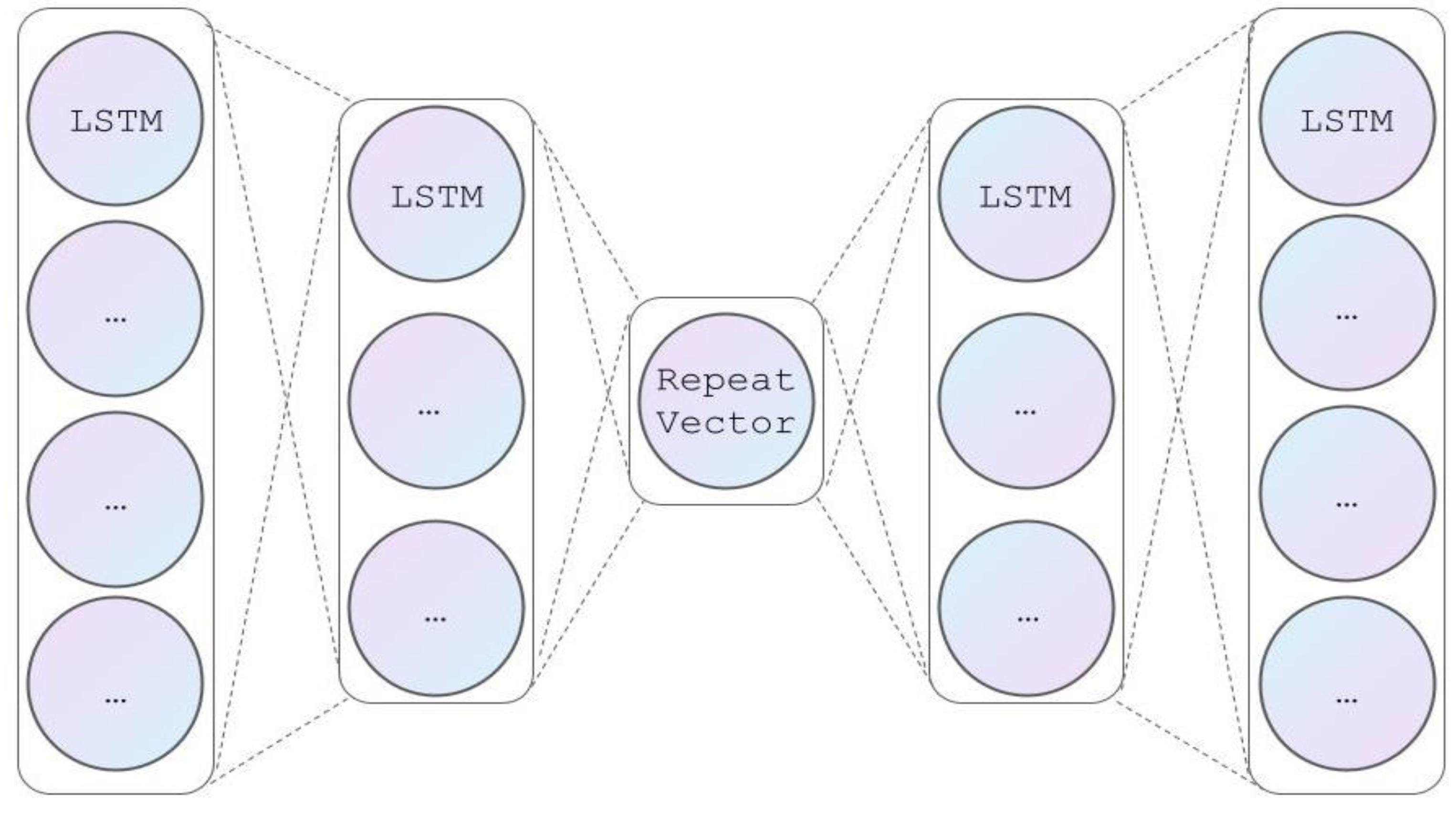
Autoencoders are multi-layer symmetrical ANN structures often used in conjunction with LSTM neural networks. In a typical multi-sensor anomaly detection, the relative value of each variable is not known a priori, and the datasets are typically unlabeled. Autoencoders offer advantages in pattern recognition of unlabeled data sets, as they prioritize the learning of the best encoding–decoding scheme from the data. An input layer feeds data into the encoder, which compresses information by passing it through increasingly smaller neural network hidden layer depths. The decoder decompresses the encoded representation into the output layer, which recreates the input data. The encoding and decoding processes force the model to learn reconstruction of the data, where the essential features of the input values are extracted. Thus, the model learns the patterns in data without the need to manually specify the inputs and the outputs. A schematic diagram of the autoencoder architecture is shown in Figure 2.
For the problem in this study, the input consists of time series of all sensors. During training, the reconstructed output is compared with the actual values. Performance of the model is evaluated with the loss function, which we calculate as the combined Mean Absolute Error (MAE) across all of the sensors:
Here, Yi is the prediction, Xi is the true value, and n is the number of sensors. The residual between these two values is known as the error or loss. Another common loss function is the Mean Squared Error (MSE).
In comparison to MAE, MSE could excessively punish outlier data, which would diminish model performance in anomaly detection applications. Analyzing statistical loss distribution for the training data, one selects the threshold value for anomaly detection. During monitoring, an anomaly is reported if the loss is larger than the threshold. To achieve optimal performance sensitivity (detection of anomaly) and specificity (reduction of false alarms), training data should capture maximum variance of the system operating range. Because learning is a statistical process, in practice, this can be accomplished by acquiring larger volumes of training data. The learning process could be iterative, with additional training data acquired pending intermediate performance results.
3. Data Acquisition in Liquid Sodium Purification System Cold Trap
3.1. Cold Trap Purification System
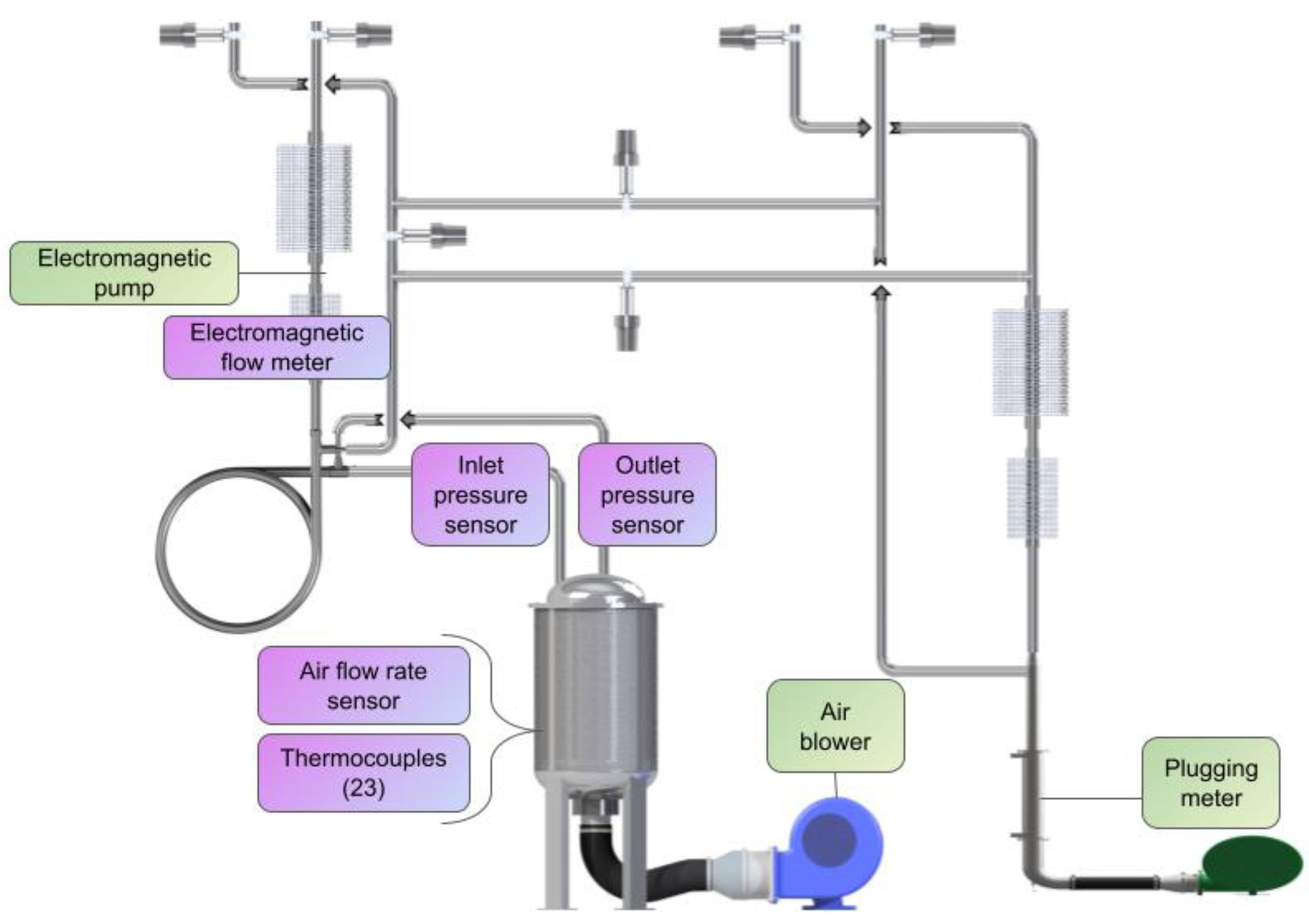
Anomaly detection study in this paper was investigated using data obtained from an experiment performed at the Mechanisms Engineering Test Loop (METL) liquid sodium facility at Argonne National Laboratory [40]. The METL facility is equipped with a purification and diagnostic system that consists of a cold trap, a plugging meter, an economizer, two EM (electromagnetic) pumps, two flowmeters, and four pressure transducers. A schematic diagram of the purification system is depicted in Figure 3. All components in the purification system are rated for temperatures up to 538 °C (1000 °F) and pressures ranging from 0.01 Pa to 0.7 MPa, in accordance with the ASME codes.
The purification system at METL is designed to work in four different operational modes: (1) Purification mode—only the cold trap is in use. This mode can be used after a test article has been inserted or removed since there could be a higher impurity concentration and a greater likelihood of clogging the plugging meter. (2) Measuring mode—only the plugging meter is in use. This mode can only be used to monitor the impurity levels within the flowing sodium. (3) Purification/Measuring mode—both the cold trap and the plugging meter are in use while connected to the main loop in parallel. This mode may be used to simultaneously clean and monitor the bulk sodium. (4) Test mode—both the cold trap and the plugging meter are connected in series. This mode can be used to determine the effectiveness of the cold trap at different temperatures and flow rates. A similar purification and diagnostic system could be implemented in a commercial SFR [41].
The cold trap operates by cooling a small fraction of the flow in the main piping system to temperatures just above the freezing point of sodium. At these colder temperatures, the solubility of oxides, hydroxides, or other impurities is drastically reduced. If dirty sodium enters the cold trap, sodium becomes super saturated with the impurities as the liquid is cooled. The impurities are then precipitated out of solution and adhere to the stainless-steel mesh packing within the volume of the cold trap. The clean, cool sodium can then reenter the main loop as the cleaning process continues. To cool the sodium, the cold trap loop relies on both an economizer and a blower to push ambient air over the cold trap’s heat transfer fins. Cold Trap Design Parameters are listed in Table 1. The components of the purification system reduce sodium temperatures from a maximum of 538 °C/1000° F to the plugging temperature 110–150 °C at a nominal flow rate of 1 gpm (gallons per minute). The objective of the purification system is to reduce oxygen and hydrogen impurity concentrations to levels below 5 ppm (parts per million).
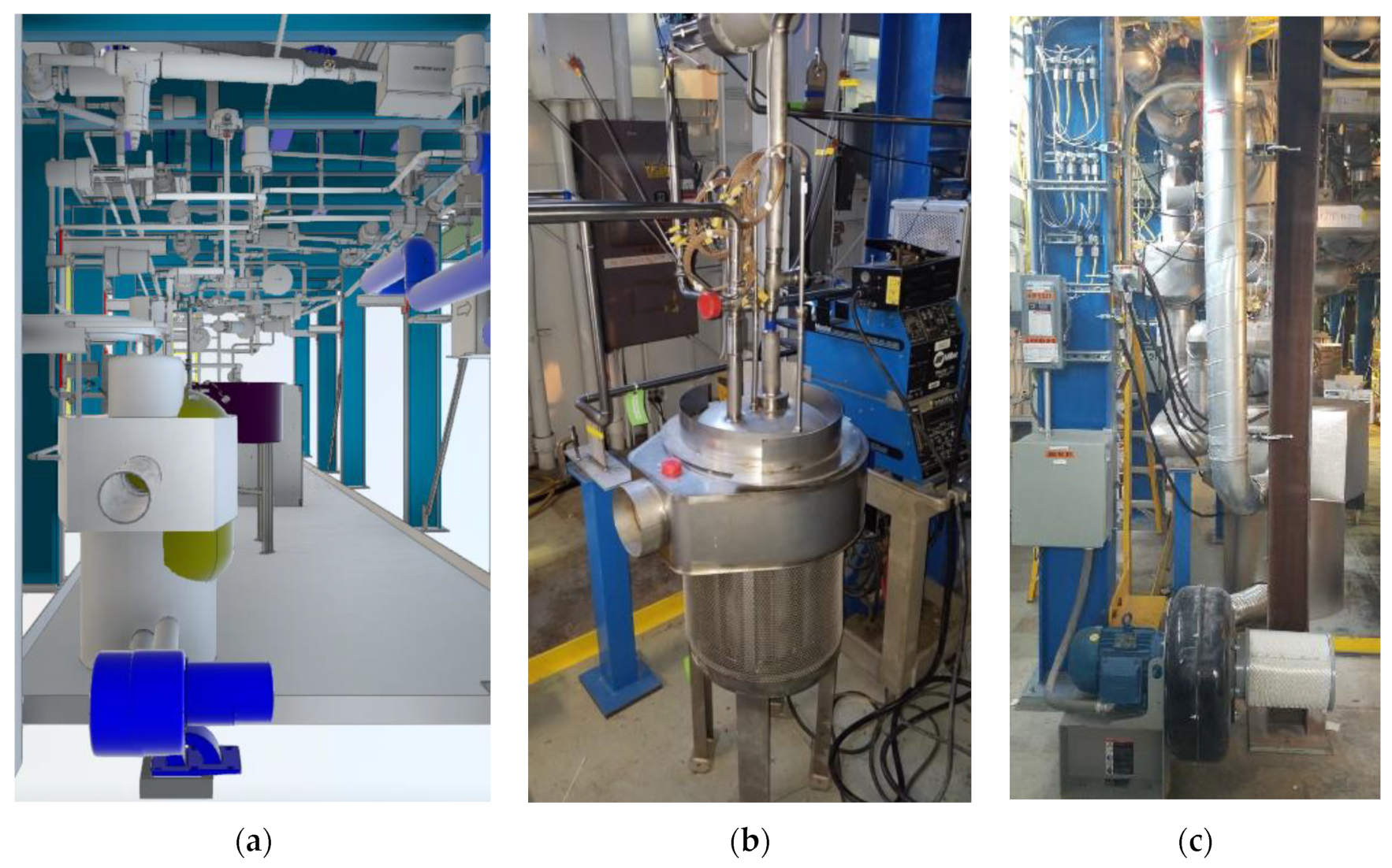
Figure 4a shows a 3D rendering of the cold trap, and Figure 4b,c contain photographs of the system taken from different angles. The blower delivers ambient air to the bottom of the cold trap. The air absorbs heat from the cold trap, which is filled with molten sodium. The air is then exhausted through the top duct.
For the input layer to the autoencoder, we used 31 dynamic variables involved in monitoring of the cold trap. Of these variables, 29 are sensor measurements of sodium and air temperatures, flow rates and pressures, and two are PID (proportional integral derivative) controller signals that provide information about the electromagnetic (EM) pump and air blower speed. The details of the dynamic variables are summarized in Table 2. The most common sensors in the cold trap are type-K thermocouples housed in a probe welded to the top of the cold trap vessel, so that they are in contact with the flowing sodium. Inlet and outlet pressures of the cold trap are measured with pressure transmitters to monitor the amount of contamination retained in the cold trap. A blower that delivers cooling air to the cold trap is equipped with a variable frequency drive (VFD). The PID signals for air blower and EM pump are relative percentages of frequency of VFD and applied voltage, respectively.
3.2. Cold Trap Anomaly Generation Experiment and Data Acquisition
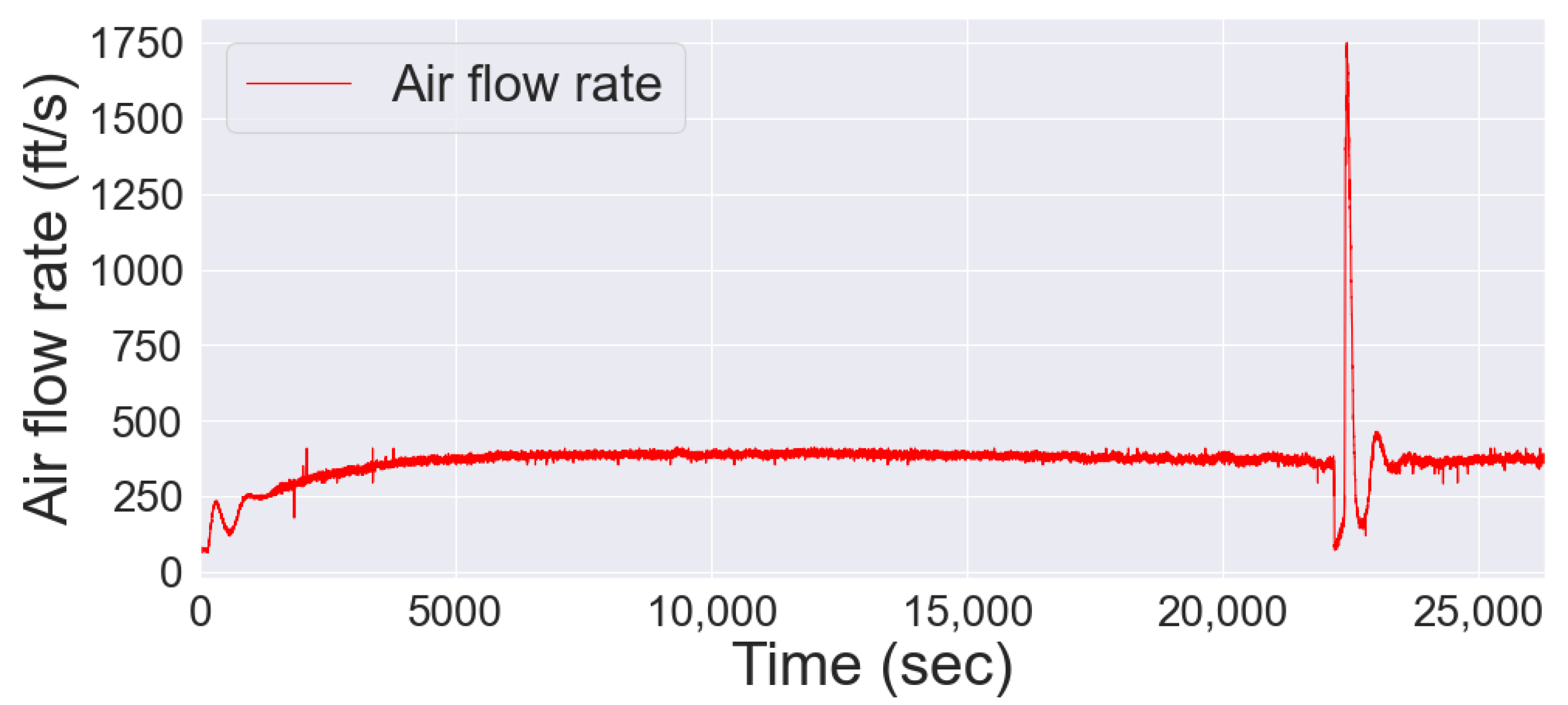
The dataset of 31 variables involved in dynamic monitoring of the cold trap operation was collected over the course of seven hours on the same day. The total measurement time is 26,303 s, with data sampled every 0.15 s, resulting in 175,100 data points for each of 31 variables. As examples of recorded data, Figure 5 displays time series of the blower flow rate, and Figure 6 shows the times series of eight thermocouples in the center of the cold trap. Approximately the first 5000 s consist of the cold trap startup transient, during which sensor readings show initial oscillatory response followed by a gradual rise in amplitude. The time segment between approximately 5000 s and 22,000 s corresponds to normal cold trap operation.
Process disturbance or an anomaly signal was created starting at time instance 22,168 s, with a total time duration of approximately 1200 s. The anomaly signal in this study was generated by unplugging the flow damper and choking the air blower. This caused a temperature spike, which in turn resulted in a spike in the air blower speed as the system tried to correct itself to maintain stability. Closing the damper, the air flow rate in the blower in the cold trap decreased from 400 ft/s to 60 ft/s, as shown in Figure 5. The blower rate then increased to 1750 ft/s to maintain normal operations, resulting in a subsequent spike in liquid sodium temperature that can be seen in Figure 6. The largest temperature spike is 3.7 °C registered with Thermocouple 1 (blue curve). The simulated malfunction of the damper in the cold trap in METL is representative of a potential loss of coolant for a cold trap in the breeder-type SFR [3], such as an accidental closure of a valve, or an obstruction in a pipe.
We observed that anomaly signal was registered in time series of the 26 variables, which include blower temperature, blower speed, air flow rate, and all thermocouples values. However, because the anomaly detection approach is agnostic to data, we have included all 31 cold trap variables in the autoencoder development.
4. Results of Anomaly Detection in Cold Trap
4.1. Training of LSTM Autoencoder
The LSTM autoencoder model was built with the Keras API (Application Programming Interface) using the Adams optimizer. The dataset of 26,303 s for each of 31 variables in the cold trap system was split evenly between training and testing data sets, with 5% of the training data reserved for model validation. The 31 variables involved in monitoring the cold trap in the METL Facility constitute the input layer of the LSTM autoencoder. The variable values were scaled to be in the range between 0 and 1, so that sensors with higher nominal measurement values do not dominate other sensors. The input layer was compressed by gradually reducing the number of hidden neurons, from 16 neurons to 4 neurons, in two additional layers of the encoder. A repeat vector layer was positioned in the middle of the autoencoder. The decoder containing expanding layers gradually increased hidden neurons size. The final output layer of the decoder has the same dimension as the input layer, thus providing a reconstruction of all 31 cold trap variables.
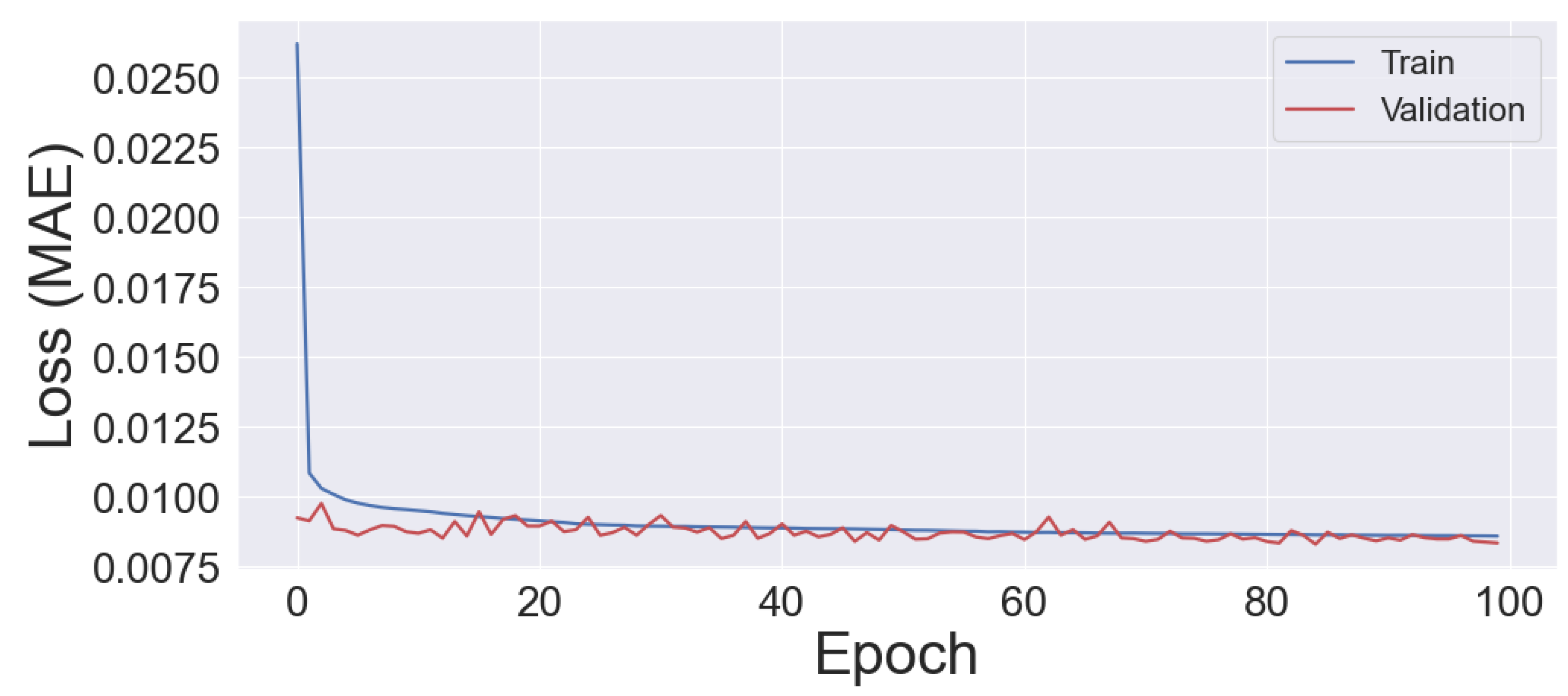
The LSTM autoencoder model trained for 100 epochs with a learning rate of 0.001. Training of the LSTM autoencoder took 36 min and 43 s on an Intel Core i5-3570S CPU processor with 16 GB of RAM. The learning curve showing the losses for training and validation data is shown in Figure 7.
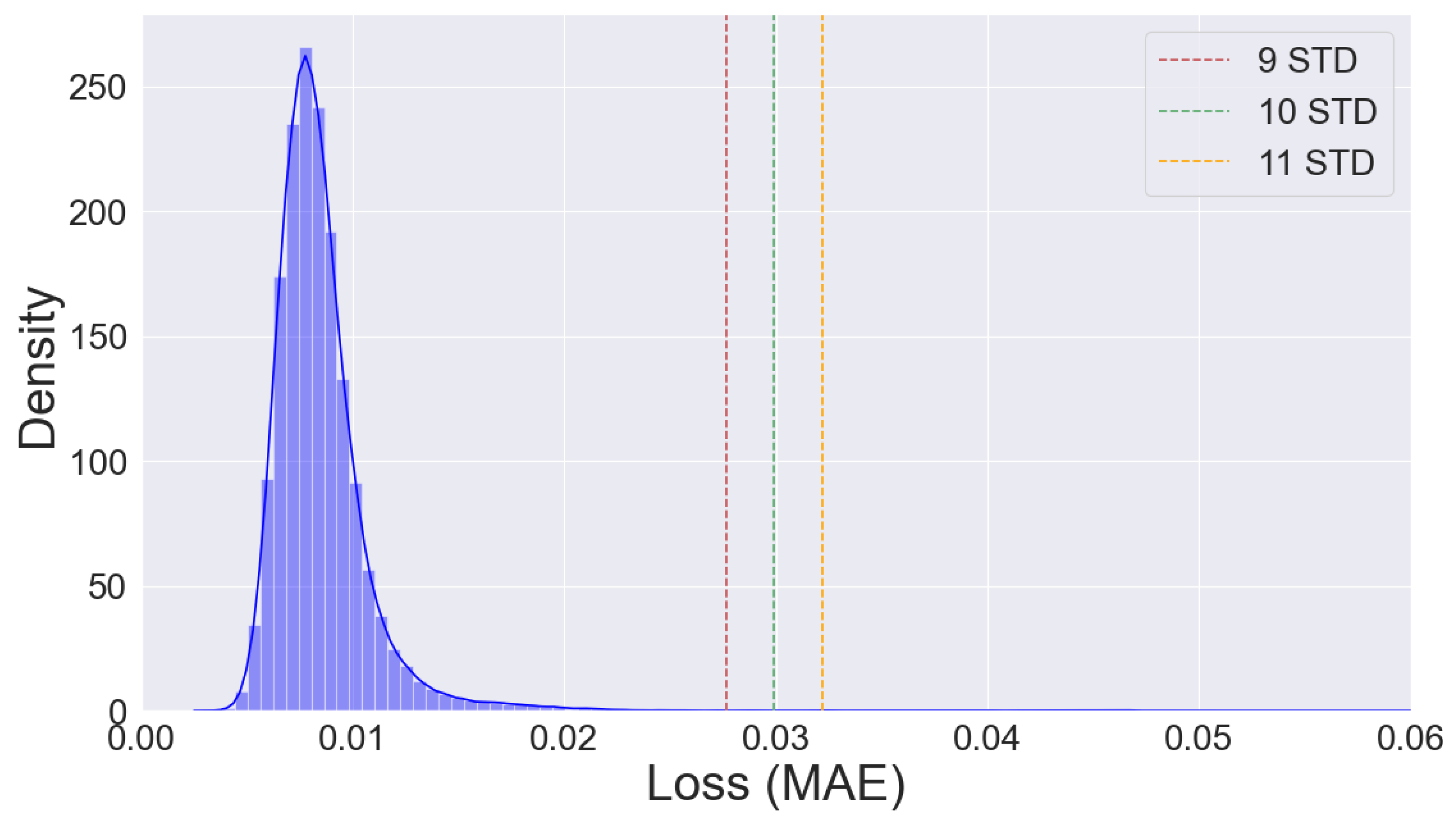
Density distribution (histogram) of the training loss, calculated as MAE, is plotted in Figure 8. From this graph, we have determined the loss is described by log-normal distribution with parameters µ and σ.
The mean value and standard deviation of log-normal distribution are given as
Fitting the log-normal model to LSTM autoencoder loss density distribution, we determined the parameters values µ = −4.971, σ = 0.332, Mean = 0.0073, and STD = 0.0025. Three different thresholds for anomaly detection indicated by vertical lines in Figure 8 were chosen at 9 STD (red), 10 STD (green), and 11 STD (yellow) from the loss mean. Note that setting the threshold at a higher value reduces the false alarm rate, but also reduces sensitivity to anomaly.
False alarm probabilities for different loss threshold values are listed in Table 3. For a given loss threshold value, the probability of a false alarm was calculated as the ratio of the area under the density curve above the threshold to the area under the density curve for the entire range.
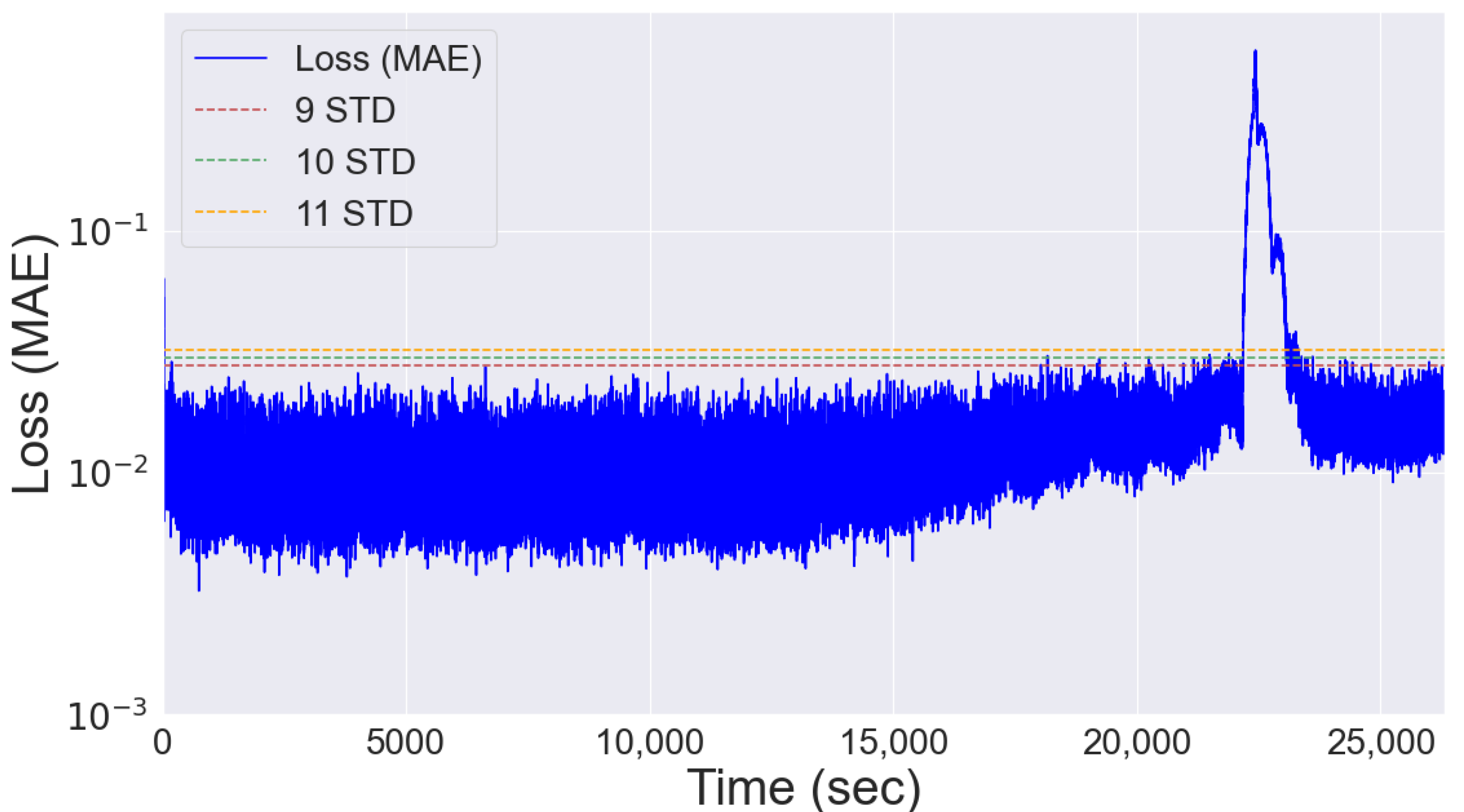
Loss for the entire data set is plotted on linear-log scale as a function of time in Figure 9. Thresholds for anomaly detection set at 9 STD, 10 STD, and 11 STD are indicated by horizontal lines, with red, green, and yellow colors. Note that prior to occurrence of anomaly caused by choking the blower, the largest loss is during the cold trap startup transient. The anomaly signal time window was estimated from Figure 9 by finding the time instant when the loss peak, which begins at 22,168 s, decreases below the threshold value of 9 STD. This gives the time of 22,375 s as the end of the anomaly signal time window.
4.2. Anomaly Signal Scaling
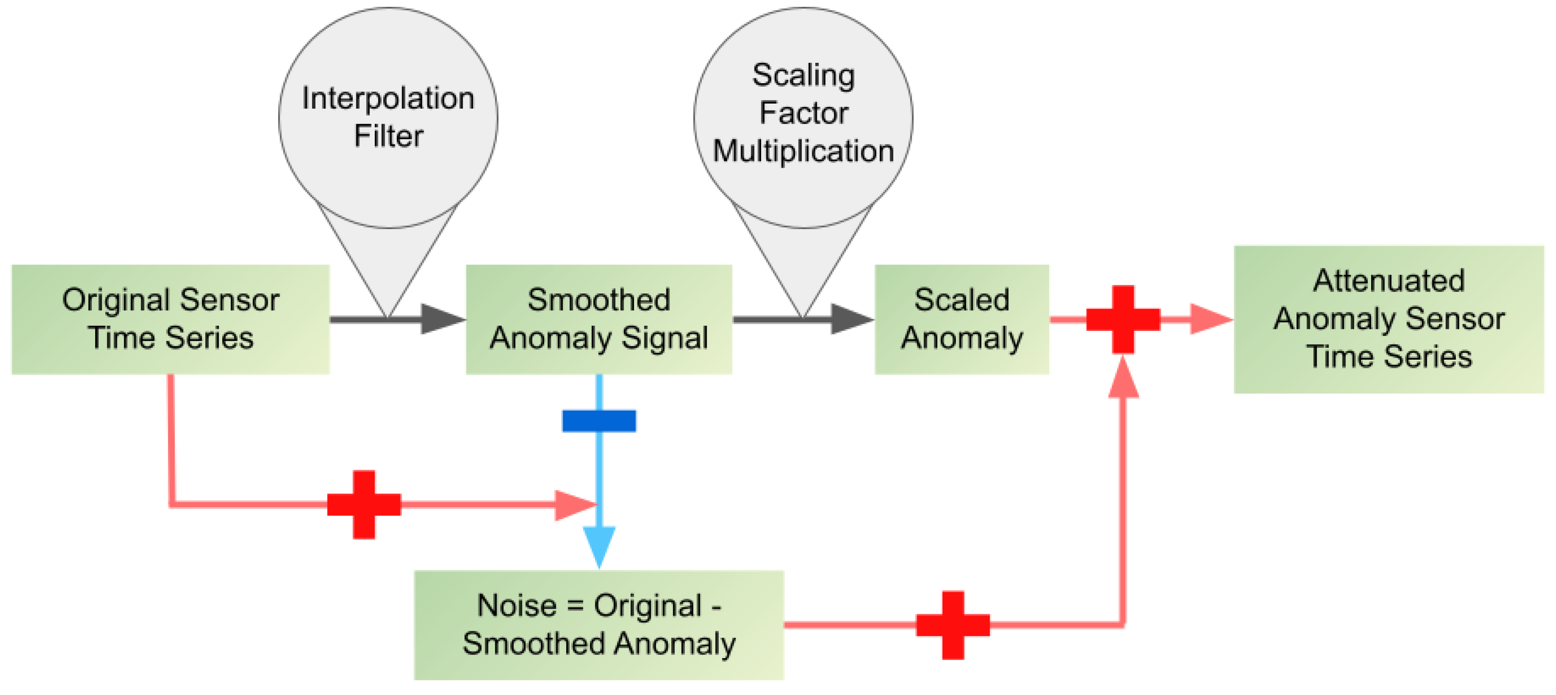
To investigate the sensitivity of the LSTM autoencoder model, we performed a parametric study in which we varied the process anomaly amplitude. The experimentally measured signal in each sensor corresponding to process anomaly was digitally reduced through a spectral filtering technique which attenuates the anomaly signal without attenuating the noise. The flow chart of the sensor anomaly attenuation algorithm is shown in Figure 10. The anomaly segment of the sensor time series was selected in a window of 3000 s. One can observe that the noise in measurements consists of high-frequency fluctuations, while the anomaly due to pump choking consists of lower frequency oscillations. An interpolation filter, which in this paper consists of 20-point smoothing spline interpolations, was applied to the experimental anomaly signal. The sampling rate during the measurements was 0.15 s, corresponding to a 6.67 Hz frequency bandwidth. Interpolation increases the sampling rate to 3 s, which suppresses frequencies below 0.33 Hz. The smoothed signal was subtracted from the original to obtain the noise component of the original data. The smoothed anomaly signal was multiplied by the scaling factor to obtain a scaled anomaly. In this paper, scaling factors consisted of integer powers of ½, with the smallest multiplicative factor of 1/32. Finally, noise was added to the scaled anomaly to obtain scaled anomaly with the same noise component as that in the original measurement data. The time window containing scaled anomaly was then merged into the testing dataset. The same procedure was applied to scaling the anomaly amplitude of all 31 sensors in the cold trap.
Scaled process anomaly is characterized with the signal-to-noise ratio metric (SNR). The SNR for each sensor is calculated as the ratio of mean (expectation) values of squares of smoothed anomaly signal and noise signal for this sensor:
The SNR for the process anomaly was obtained by averaging SNR values across all sensors.
An example of anomaly signal attenuation by a factor of 1/32 in the blower air flow rate is shown in Figure 11. For this scaling factor, the anomaly SNR = 0.67 (averaged across all sensors). Note that the noise component is similar in the original and scaled anomaly time series. The power spectrum of the original and scaled flow rate, calculated with Fast Fourier Transform numerical routine, is shown in Figure 12. Note that the frequencies below 0.33 Hz are attenuated in the scaled signal, while the frequency components above 0.33 Hz are nearly the same in both the scaled and original anomaly signal. Similar attenuation of low frequency components in scaled anomaly signals was verified for different scaling coefficients, from 1/2 to 1/32.
Time series of the loss with the anomaly signal scaled by a factor of 1/32 are plotted in Figure 13. The time window of the anomaly signal, starting at 22,168 s and ending at 23,375 s, is indicated in Figure 13 with vertical black and purple lines. The loss thresholds at 9 STD, 10 STD, and 11 STD from the mean are indicated with yellow, green, and red lines, respectively.
Table 4 presents a summary of LSTM autoencoder performance in detection of anomaly signals with different amplitudes and for different loss threshold values. For each anomaly case, all sensor values were attenuated by a scaling factor, which are integer powers of ½, with the smallest value of 1/32 listed in the first column of Table 4. Anomaly SNR listed in the second column of Table 4 was calculated by averaging SNRS across all 31 cold trap variables. The third column of Table 4 lists time to detect anomaly (when the anomaly loss exceeds the threshold value) for loss threshold values at 9 STD, 10 STD, and 11 STD from the mean. The time to detect anomaly is counted from the time instant of 22,168 s, when the process anomaly was initiated by choking the blower.
One can observe that the time to detect the anomaly, for the same value of SNR, increases with the value of loss threshold. For a fixed value of loss threshold, the anomaly detection time increases with a decreasing SNR value. The smallest value of anomaly SNR for which the LSTM autoencoder reports detection is SNR = 0.67 (anomaly scaling by factor 1/32). However, the maximum loss threshold for which detection is achievable is 10 STD, and time to detect the anomaly is 186 s or approximately 3 min. LSTM autoencoder was unable to detect the anomaly for SNR = 0.17 for loss threshold set 9 STD and above.
5. Discussion
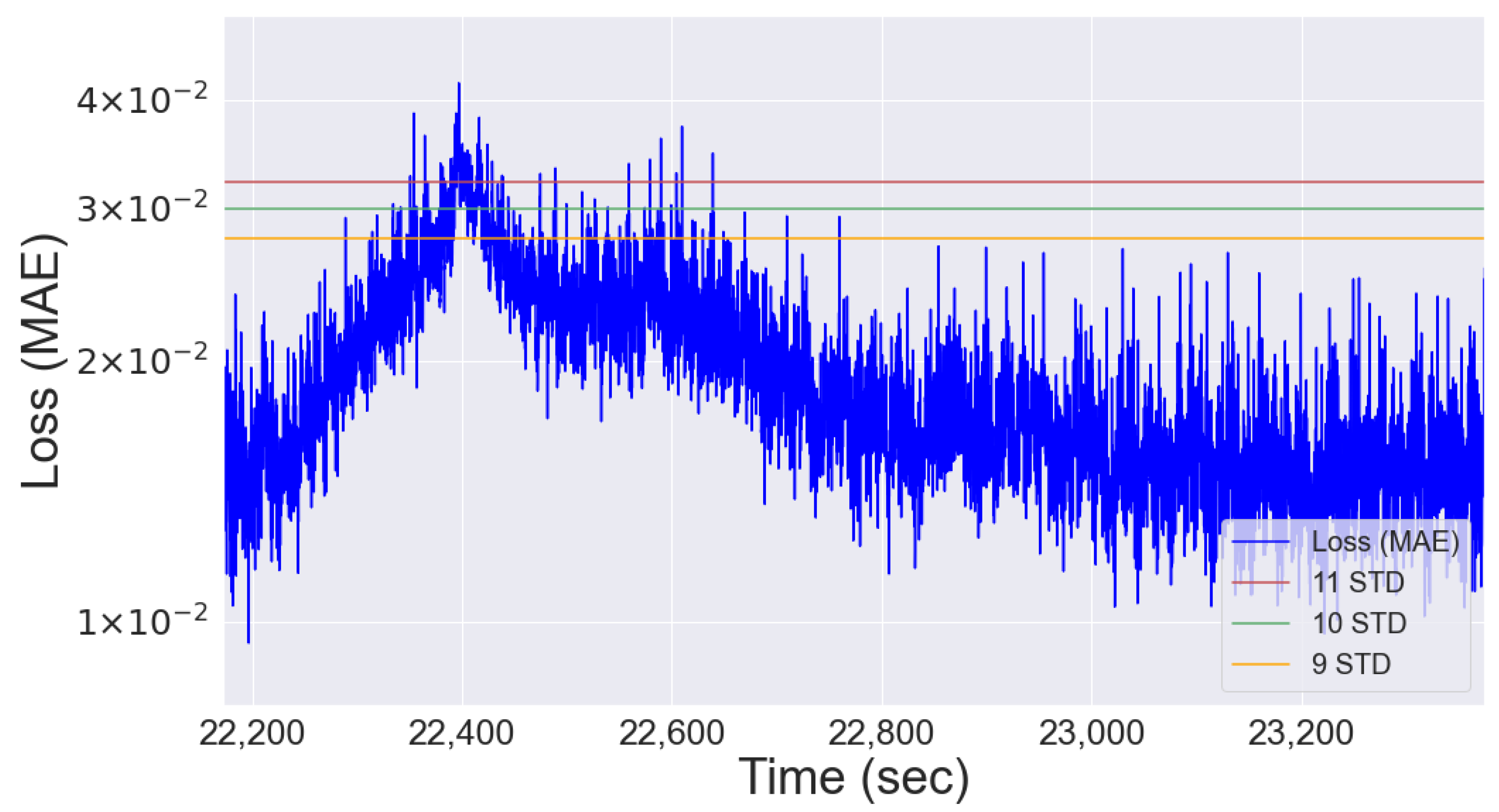
The approach to anomaly detection in this paper consists of selecting a loss threshold value using statistical distribution of loss obtained with autoencoder training data. To minimize false alarms, we chose threshold values of 9 STD, 10 STD, and 11 STD from the mean, which are expected to have a probability of false alarms smaller than 0.3%. To further examine performance of this approach for attenuated anomaly values, we plot the loss time series zoomed in to the anomaly time window between 22,168 s and 23,375 s. Figure 14 displays the anomaly signal attenuated by a factor 1/16, for which SNR = 2.69. According to Table 4, an anomaly was detected for all three thresholds, with the anomaly detection time increasing with the threshold value. This is consistent with the visualization of the attenuated anomaly signal in Figure 14. The first peak in the anomaly signal, centered at approximately 22,400 s, crosses all three thresholds. The second peak in the anomaly signal is centered at approximately 22,600 s. The mean value of the second peak of the anomaly signal is below all three thresholds, but the spikes on the second peak rise above the thresholds several times.
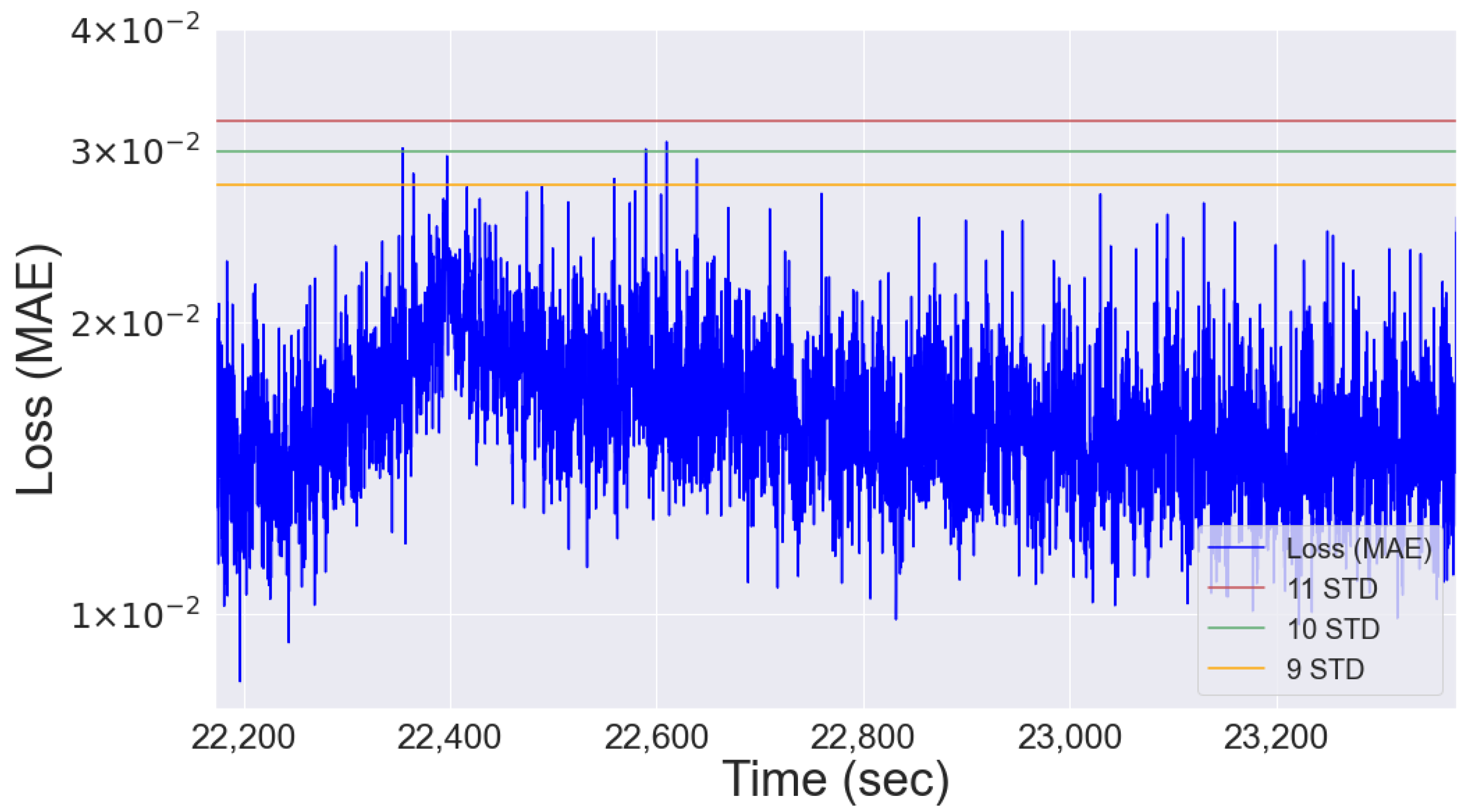
Figure 15 displays the anomaly signal attenuated by a factor of 1/32, for which SNR = 0.67. According to Table 4, the anomaly was detected at the same time with 9 STD and 10 STD thresholds, but never detected for the 11 STD threshold. We observe in Figure 15 that the average value of the loss is below the threshold of 9 SDT. Anomaly detection reported in Table 4 corresponds to sporadic spikes crossing the thresholds of 9 STD and 10 STD. The spikes have a temporal duration of 0.15 s sampling rate and appear because of measurements noise. The first crossing of the 9 STD and 10 STD threshold occurs at approximately 22,350 s or 186 s after the start of the anomaly signal. The spikes crossing the anomaly threshold are the noise on top of the first anomaly signal peak at 22,400 s. The spikes cross the 9 SDT and 10 SDT thresholds twice more at approximately 22,600 s, which is the center of the second peak of the anomaly signal.
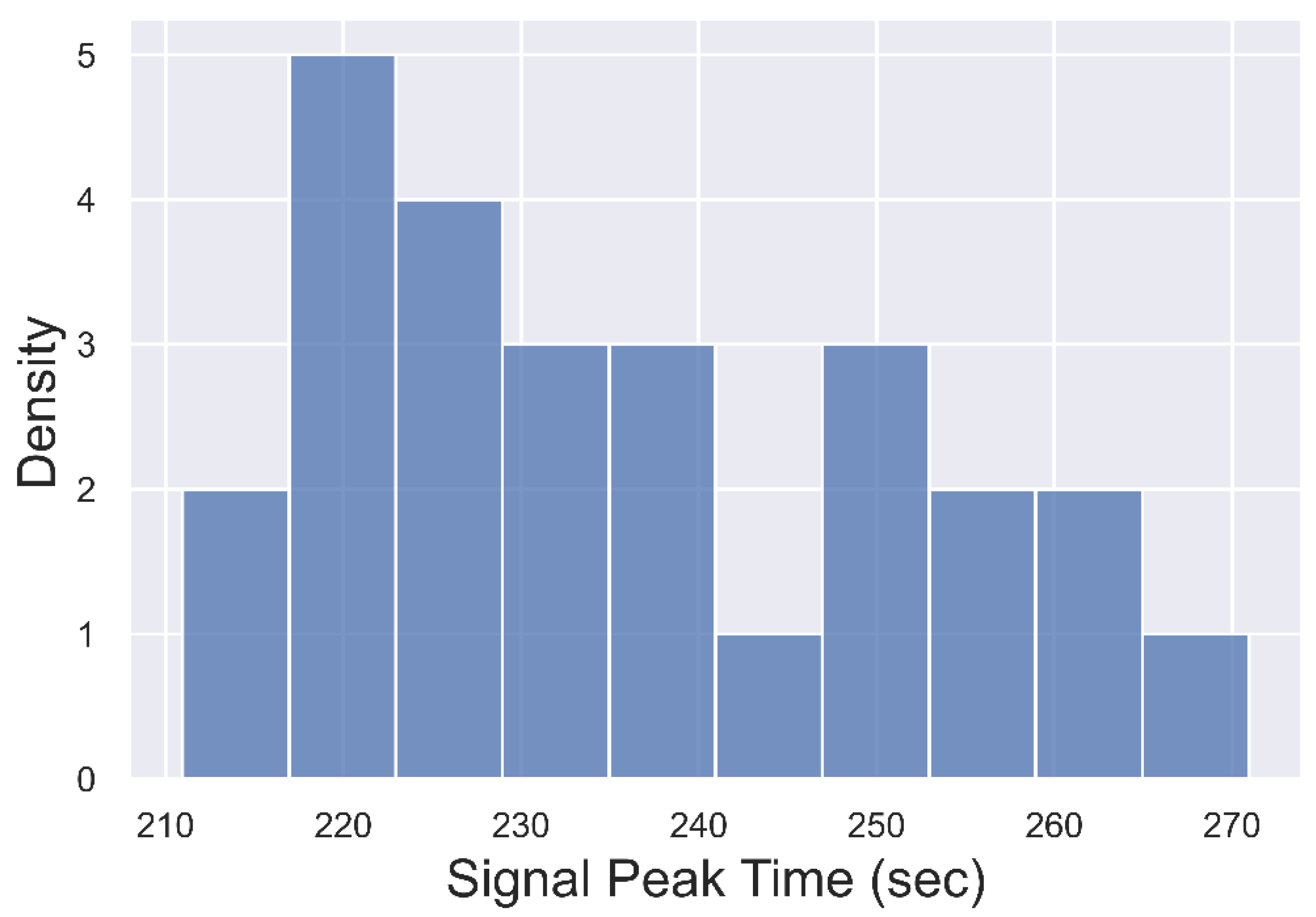
Another factor affecting performance of the anomaly detection scheme in this work is the fact that individual anomaly signals, appearing in 26 variables involved in monitoring the cold trap, have different pulse shapes with peak values at different times. The delays in signal peaks occur because the anomaly in the cold trap involves a chain of events that sequentially propagate through the system. In addition, sensors at different spatial locations in the cold trap register anomaly signals at different times. Distribution of anomaly signals peak times, as measured after the start of the anomaly at 22,168 s, is plotted in Figure 16. The peak times of anomaly signals are continuously distributed between 212 s and 267 s. The distribution has a bi-modal shape, with the first maxima of the histogram at approximately 225 s, and the second maxima at approximately 260 s. Since the peaks of anomaly signals are distributed over a time span of 55 s, the loss calculated as MAE is broadened, with a corresponding reduction of the loss peak.
In future work, we will consider a criterion for anomaly detection, which will require the anomaly signal to continuously exceed the threshold value for a specified time period. With that approach, the threshold for anomaly detection could be selected at a lower value than the ones in the present study. This could allow distinguishing between anomaly and sporadic events potentially corresponding to false alarms. In addition, we will consider strategies for anomaly detection that take into account time delays in signal peaks of cold trap variables. One approach could involve coincidence detection, where an anomaly detection in one variable would be conditioned on anomaly detection within a specified time window in other variables in the cold trap. This approach could also help to discriminate between a process anomaly and a sensor failure. The former would be registered by multiple variables in the cold trap, while the latter would result in a single anomalous signal.
6. Conclusions
We have investigated data-driven process anomaly detection in the cold trap of a liquid sodium purification system using an LSTM autoencoder model trained on startup and steady state operation data. The cold trap was monitored with 31 sensors, which included temperature, flow, and pressure of liquid sodium and air. The total measurement time is 26,303 s, with data sampled every 0.15 s, resulting in 175,100 data points for each sensor. An anomaly was generated by unplugging a damper and choking the air blower, which created temperature and flow spikes. This anomaly is representative of a loss coolant in a cold trap of an SFR. The structure of the LSTM autoencoder has the capacity to fuse multi-stream data. By performing data compression and decompression, the autoencoder learns about the patterns of data during training. The input layer to the autoencoder consisted of normalized time series of 31 sensors. Learning of the autoencoder is achieved via minimization of loss, which is calculated as minimum average error (MAE) across all sensors. We determined that the density distribution of the loss for the training data is log-normal, with the mean value of 0.0073, standard deviation of 0.0025, and the largest value of 0.06. During monitoring, the anomaly is detected if the loss for the anomaly exceeds a pre-defined threshold value. Thus, accuracy of the LSTM autoencoder performance depends on the availability of the training data that allows one to construct loss density distribution and select the appropriate threshold value
To investigate sensitivity to anomaly detection, we scaled experimentally measured anomaly signals in each sensor using a procedure that attenuates the low frequency anomaly signal but preserves high-frequency sensor noise. We calculated the signal-to-noise ratio (SNR) for the anomaly signal for each sensor and averaged across all sensors to obtain SNR for the anomaly. For sensitivity analysis, we chose several loss threshold values, measured at 9 STD, 10 STD, and 11 STD from the mean. The probability of a false alarm increases with the decreasing value of the threshold. For threshold values considered in this study, probability of false alarm is less than 1%. Our study has shown that process anomaly with SNR < 1 can be detected after approximately 3 min from the instance of process anomaly initiation.
In this paper, we considered any event of the autoencoder loss exceeding the threshold value to constitute an anomaly. In future work, we will develop new criteria for anomaly detection by requiring that the signal remain continuously above the threshold value for a minimal period of time. This should help with discriminating between process anomalies and random events of spikes due to measurement noise rising above the detection threshold. In addition, we have observed that the anomaly signal peaks of variables involved in monitoring the cold are distributed over a time interval of approximately 50 s. The lag in signals decreased the SNR of the loss, which is calculated as MAE. In future work, we will incorporate spatial and temporal correlations between sensors, such as coincidence detection, into calculation of loss. Future work will also investigate process anomaly detection in the presence of sensor faults, such as drift. Since the objective is to detect process anomaly, sensor fault will be classified as a false alarm.
Author Contributions
Conceptualization, A.A., D.K. and A.H.; methodology, A.A., D.K. and A.H.; software, A.A.; validation, A.A. and A.H.; formal analysis, A.A. and A.H.; investigation, A.A. and A.H.; resources, D.K. and A.H.; data curation, A.A. and D.K.; writing—original draft preparation, A.A.; writing—review and editing, A.H.; visualization, A.A.; supervision, A.H.; project administration, A.H.; funding acquisition, A.H. All authors have read and agreed to the published version of the manuscript.
Funding
This work was supported by the U.S. Department of Energy, Advanced Research Projects Agency—Energy (ARPA-E) under contract DE-AC02-06CH11357.
Data Availability Statement
The data presented in this study are available on request from the corresponding author.
Acknowledgments
The dataset in this paper was obtained from an experiment conducted at the Mechanisms Engineering Test Loop (METL) Facility at Argonne National Laboratory.
Conflicts of Interest
The authors declare no conflict of interest.
References
- Sofu, T. A review of inherent safety characteristics of metal alloy sodium-cooled fast reactor fuel against postulated accidents. Nucl. Eng. Technol. 2015, 47, 227–239. [Google Scholar] [CrossRef] [Green Version]
- Rodriguez, G.; Varaine, F.; Costes, L.; Venard, C.; Serre, F.; Chanteclair, F.; Chenaud, M.-S.; Dechelette, F.; Hourcade, E.; Plancq, D.; et al. France–Japan Synthesis Concept on Sodium-Cooled Fast Reactor Review of a Joint Collaborative Work. EPJ Nucl. Sci. Technol. 2021, 7, 15. [Google Scholar] [CrossRef]
- Holmes, J.T.; Smith, C.R.F.; Osterhout, M.M.; Olson, W.H. Sodium Purification by Cold Trapping at the Experimental Breeder Reactor II. Nucl. Technol. 1977, 32, 304–314. [Google Scholar] [CrossRef]
- Kozlov, F.A.; Sorokin, A.P.; Konovalov, M.A. Sodium Purification Systems for NPP with Fast Reactors (Retrospective and Perspective Views). Nucl. Eng. Technol. 2016, 2, 5–13. [Google Scholar] [CrossRef] [Green Version]
- Kim, K.R.; Jeong, J.Y.; Jeong, K.C.; Kwon, S.W.; Hwang, S.T. Theoretical Analysis of the Sodium Purification for Cold Trap Design and Performance Measurement. J. Ind. Eng. Chem. 1998, 4, 113–121. [Google Scholar]
- Kim, H.; Kim, J.-T.; Eoh, J.; Lim, D.-W. Development of a Physics-Based Monitoring Algorithm Detecting CO2 Ingress Accidents in a Sodium-Cooled Fast Reactor. Energies 2018, 12, 1. [Google Scholar] [CrossRef] [Green Version]
- Heifetz, A.; Vilim, R.B. Eigendecomposition Model of Resistance Temperature Detector with Applications to S-CO2 Cycle ensing. Nucl. Eng. Des. 2017, 311, 60–68. [Google Scholar] [CrossRef] [Green Version]
- Fink, J.K.; Liebowitz, L. Thermodynamic and Transport Properties of Sodium Liquid and Vapor; ANL/RE-95/2; Argonne National Laboratory: Lemont, IL, USA, 1995. [Google Scholar]
- Gao, J.; Li, P.; Chen, Z.; Zhang, J. A Survey on Deep Learning for Multimodal Data Fusion. Neural Comput. 2020, 32, 829–864. [Google Scholar] [CrossRef]
- Nikiforov, I.; Harrou, F.; Cogranne, R.; Beauseroy, P.; Grall, E.; Guépié, B.K.; Fillatre, L.; Jeannot, J.-P. Sequential Detection of a Total Instantaneous Blockage Occurred in a Single Subassembly of a Sodium-Cooled Fast Reactor. Nucl. Eng. Des. 2020, 366, 110733. [Google Scholar] [CrossRef]
- Martinez-Martinez, S.; Messai, N.; Jeannot, J.-P.; Nuzillard, D. Two Neural Network Based Strategies for the Detection of a Total Instantaneous Blockage of a Sodium-Cooled Fast Reactor. Reliab. Eng. Syst. 2015, 137, 50–57. [Google Scholar] [CrossRef]
- Tasakos, T.; Ioannou, G.; Verma, V.; Alexandridis, G.; Dokhane, A.; Stafylopatis, A. Deep Learning-Based Anomaly Detection in Nuclear Reactor Cores. In Proceedings of the International Conference on Mathematics & Computational Methods Applied to Nuclear Science & Engineering (M&C 2021), Online, 3–7 October 2021; pp. 3–7. [Google Scholar]
- Calivá, F.; De Sousa Ribero, F.; Mylonakis, A.; Demaziere, C.; Vinai, P.; Leontidis, G.; Kollias, S. A Deep Learning Approach to Anomaly Detection in Nuclear Reactors. In Proceedings of the 2018 International Joint Conference on Neural Networks (IJCNN), Rio de Janeiro, Brazil, 8–13 July 2018; pp. 1–8. [Google Scholar]
- Gohel, H.A.; Upadhyay, H.; Lagos, L.; Cooper, K.; Sanzetenea, A. Predictive Maintenance Architecture Development for Nuclear Infrastructure Using Machine Learning. Nucl. Eng. Technol. 2020, 52, 1436–1442. [Google Scholar] [CrossRef]
- Santos, M.C.; Pereira, C.M.N.A.; Schirru, R. A Multiple-Architecture Deep Learning Approach for Nuclear Power Plants Accidents Classification Including Anomaly Detection and “Don’t Know” Response. Ann. Nucl. Energy 2021, 162, 108521. [Google Scholar] [CrossRef]
- Prantikos, K.; Tsoukalas, L.H.; Heifetz, A. Physics-Informed Neural Network Solution of Point Kinetics Equations for a Nuclear Reactor Digital Twin. Energies 2022, 15, 7697. [Google Scholar] [CrossRef]
- Akins, A.; Wu, X. Using Physics-Informed Neural Networks to solve a System of Coupled Nonlinear ODEs for a Reactivity Insertion Accident. In Proceedings of the 2022 International Conference on Physics of Reactors, Pittsburg, PA, USA, 15–20 May 2022. [Google Scholar]
- Al Rashdan, A.Y.; Abdel-Khalik, H.S.; Giraud, K.M.; Cole, D.G.; Farber, J.A.; Clark, W.W.; Alemu, A.; Allen, M.C.; Spangler, R.M.; Varuttamaseni, A. A Qualitative Strategy for Fusion of Physics into Empirical Models for Process Anomaly Detection. Energies 2022, 15, 5640. [Google Scholar] [CrossRef]
- Kim, M.; Ou, E.; Loh, P.-L.; Allen, T.; Agasie, R.; Liu, K. RNN-Based Online Anomaly Detection in Nuclear Reactors for Highly Imbalanced Datasets with Uncertainty. Nucl. Eng. Des. 2020, 364, 110699. [Google Scholar] [CrossRef]
- Hochreiter, S.; Schmidhuber, J. Long Short-Term Memory. Neural Comput. 1997, 9, 1735–1780. [Google Scholar] [CrossRef]
- Pantopoulou, S.; Ankel, V.; Weathered, M.T.; Lisowski, D.D.; Cilliers, A.; Tsoukalas, L.H.; Heifetz, A. Monitoring of Temperature Measurements for Different Flow Regimes in Water and Galinstan with Long Short-Term Memory Networks and Transfer Learning of Sensors. Computation 2022, 10, 108. [Google Scholar] [CrossRef]
- Ankel, V.; Pantopoulou, S.; Weathered, M.; Lisowski, D.; Cilliers, A.; Heifetz, A. Monitoring of thermal mixing Tee sensors with LSTM neural networks. In Proceedings of the 12th Nuclear Plant Instrumentation, Control and Human-Machine Interface Technologies (NPIC-HMIT2021), Providence, RI, USA, 14–17 June 2021; pp. 313–323. [Google Scholar]
- Durrant, A.; Leontidis, G.; Kollias, S. 3D Convolutional and Recurrent Neural Networks for Reactor Perturbation Unfolding and Anomaly Detection. EPJ Nucl. Sci. Technol. 2019, 5, 20. [Google Scholar] [CrossRef]
- Pashoutani, S.; Zhu, J.; Sim, C.; Won, K.; Mazzeo, B.A.; Guthrie, W.S. Multi-Sensor Data Collection and Fusion Using Autoencoders in Condition Evaluation of Concrete Bridge Decks. J. Infrastruct. Preserv. Resil. 2021, 2, 18. [Google Scholar] [CrossRef]
- Senanayaka, J.S.L.; Huynh, V.K.; Robbersmyr, K.G. A Robust Method for Detecton and Classification of Permanent Magnet Synchronous Motor Faults: Deep Autoencoders and Data Fusion Approach. J. Phys. Conf. Ser. 2018, 1037, 032029. [Google Scholar] [CrossRef]
- Franco, E.F.; Rana, P.; Cruz, A.; Calderón, V.V.; Azevedo, V.; Ramos, R.T.J.; Ghosh, P. Performance Comparison of Deep Learning Autoencoders for Cancer Subtype Detection Using Multi-Omics Data. Cancers 2021, 13, 2013. [Google Scholar] [CrossRef] [PubMed]
- Tziolas, T.; Papageorgiou, K.; Theodosiou, T.; Papageorgiou, E.; Mastos, T.; Papadopoulos, A. Autoencoders for Anomaly Detection in an Industrial Multivariate Time Series Dataset. Eng. Proc. 2022, 18, 23. [Google Scholar]
- Nicholaus, I.T.; Park, J.R.; Jung, K.; Lee, J.S.; Kang, D.-K. Anomaly Detection of Water Level Using Deep Autoencoder. Sensors 2021, 21, 6679. [Google Scholar] [CrossRef] [PubMed]
- Givnan, S.; Chalmers, C.; Fergus, P.; Ortega-Martorell, S.; Whalley, T. Anomaly Detection Using Autoencoder Reconstruction upon Industrial Motors. Sensors 2022, 22, 3166. [Google Scholar] [CrossRef]
- Battikh, M.S.; Lenskiy, A.A. Latent-Insensitive Autoencoders for Anomaly Detection. Mathematics 2021, 10, 112. [Google Scholar] [CrossRef]
- Zhang, M.; Jiang, S.; Cui, Z.; Garnett, R.; Chen, Y. D-VAE: A Variational Autoencoder for Directed Acyclic Graphs. In Proceedings of the Advances in Neural Information Processing Systems 32: Annual Conference on Neural Information Processing Systems 2019 (NeurIPS 2019), Vancouver, BC, Canada, 8–14 December 2019; pp. 1586–1598. [Google Scholar]
- Fährmann, D.; Damer, N.; Kirchbuchner, F.; Kuijper, A. Lightweight Long Short-Term Memory Variational Auto-Encoder for Multivariate Time Series Anomaly Detection in Industrial Control Systems. Sensors 2022, 22, 2886. [Google Scholar] [CrossRef]
- Malhotra, P.; Ramakrishnan, A.; Anand, G.; Vig, L.; Agarwal, P.; Shroff, G. LSTM-based Encoder-Decoder for Multi-sensor Anomaly Detection. In Proceedings of the ICML 2016 Anomaly Detection Workshop, New York, NY, USA, 24 June 2016. [Google Scholar]
- Ibrahim, M.; Alsheikh, A.; Awaysheh, F.M.; Alshehri, M.D. Machine Learning Schemes for Anomaly Detection in Solar Power Plants. Energies 2022, 15, 1082. [Google Scholar] [CrossRef]
- Kang, J.; Kim, C.-S.; Kang, J.W.; Gwak, J. Anomaly Detection of the Brake Operating Unit on Metro Vehicles Using a One-Class LSTM Autoencoder. Appl. Sci. 2021, 11, 9290. [Google Scholar] [CrossRef]
- Hu, D.; Zhang, C.; Yang, T.; Chen, G. Anomaly Detection of Power Plant Equipment Using Long Short-Term Memory Based Autoencoder Neural Network. Sensors 2020, 20, 6164. [Google Scholar] [CrossRef]
- Park, P.; Marco, P.D.; Shin, H.; Bang, J. Fault Detection and Diagnosis Using Combined Autoencoder and Long Short-Term Memory Network. Sensors 2019, 19, 4612. [Google Scholar] [CrossRef] [Green Version]
- Zhang, C.; Hu, D.; Yang, T. Anomaly Detection and Diagnosis for Wind Turbines Using Long Short-Term Memory-Based Stacked Denoising Autoencoders and XGBoost. Reliab. Eng. Syst. 2022, 222, 108445. [Google Scholar] [CrossRef]
- Yang, K.; Wang, Y.; Han, X.; Cheng, Y.; Guo, L.; Gong, J. Unsupervised Anomaly Detection for Time Series Data of Spacecraft Using Multi-Task Learning. Appl. Sci. 2022, 12, 6296. [Google Scholar] [CrossRef]
- Kultgen, D.; Grandy, C.; Kent, E.; Weathered, M.; Andujar, D.; Reavis, A. Mechanism Engineering Test Loop—Phase I Status Report—FY2018; Update to FY2017 Report; ANL-ART-148; Argonne National Laboratory: Lemont, IL, USA, 2018. [Google Scholar]
- Ferroni, P.; Tatli, E.; Czerniak, L.; Sienicki, J.J.; Chien, H.-T.; Momozaki, Y.; Bakhtiari, S. Modeling and Validation of Sodium Plugging for Heat Exchangers in Sodium-Cooled Fast Reactor Systems; DOE-WEC-0000611-4; Westinghouse Electric Company: Cranberry Township, PA, USA, 2016. [Google Scholar]
Figure 1.
LSTM cell structure consisting of forget, input, and output gates.

Figure 2.
Schematic diagram of an autoencoder consisting of LSTM neurons.

Figure 3.
Schematic diagram of METL purification and diagnostic system indicating major components and sensors involved in system monitoring.
Figure 3.
Schematic diagram of METL purification and diagnostic system indicating major components and sensors involved in system monitoring.

Figure 4.
(a) A 3D rendering of the METL facility cold trap; (b) Photograph of the cold trap assembly without insulation (c) Photograph of working cold trap apparatus with insulation.
Figure 4.
(a) A 3D rendering of the METL facility cold trap; (b) Photograph of the cold trap assembly without insulation (c) Photograph of working cold trap apparatus with insulation.

Figure 5.
Airflow rate in the cold trap.

Figure 6.
Temperature of liquid sodium measured by eight internal thermocouples.

Figure 7.
Learning curve of LSTM autoencoder model.

Figure 8.
Log-normal density distribution of the training loss with Mean = 0.0073 and STD = 0.0025. Three different thresholds for anomaly detection are indicated by vertical dashed lines at 9 STD (red), 10 STD (green), and 11 STD (yellow) from the mean.
Figure 8.
Log-normal density distribution of the training loss with Mean = 0.0073 and STD = 0.0025. Three different thresholds for anomaly detection are indicated by vertical dashed lines at 9 STD (red), 10 STD (green), and 11 STD (yellow) from the mean.

Figure 9.
Log-linear plot of the loss for the entire data set as function of time. Anomaly thresholds are indicated by horizontal dashed lines corresponding to 9 STD (red), 10 STD (green), and 11 STD (yellow).
Figure 9.
Log-linear plot of the loss for the entire data set as function of time. Anomaly thresholds are indicated by horizontal dashed lines corresponding to 9 STD (red), 10 STD (green), and 11 STD (yellow).

Figure 10.
Flow chart of sensor anomaly signal amplitude scaling.

Figure 11.
Example of anomaly signal amplitude scaling of blower flow rate time series. Original flow rate.
Figure 11.
Example of anomaly signal amplitude scaling of blower flow rate time series. Original flow rate.

Figure 12.
Power spectrum of blower air flow original anomaly (blue) and anomaly scaled by factor 1/32 (orange). Frequency components below 0.33 Hz are attenuated in the scaled flow power spectrum.
Figure 12.
Power spectrum of blower air flow original anomaly (blue) and anomaly scaled by factor 1/32 (orange). Frequency components below 0.33 Hz are attenuated in the scaled flow power spectrum.

Figure 13.
Loss time series with anomaly signal scaled by a factor of 1/32. Start (22,168 s) and end (23,375 s) of the anomaly time window are indicated with black and purple dashed lines.
Figure 13.
Loss time series with anomaly signal scaled by a factor of 1/32. Start (22,168 s) and end (23,375 s) of the anomaly time window are indicated with black and purple dashed lines.

Figure 14.
Loss time series zoomed in to the anomaly window between 22,168 s and 23,375 s for anomaly signal attenuated by a factor of 1/16 (SNR = 2.69).
Figure 14.
Loss time series zoomed in to the anomaly window between 22,168 s and 23,375 s for anomaly signal attenuated by a factor of 1/16 (SNR = 2.69).

Figure 15.
Loss time series zoomed in to the anomaly window between 22,168 s and 23,375 s for anomaly signal attenuated by a factor of 1/32 (SNR = 0.67).
Figure 15.
Loss time series zoomed in to the anomaly window between 22,168 s and 23,375 s for anomaly signal attenuated by a factor of 1/32 (SNR = 0.67).

Figure 16.
Distribution of anomaly signal peak times of 26 variables involved in cold trap monitoring. Peak times are measured after the start of the anomaly at 22,168 s.
Figure 16.
Distribution of anomaly signal peak times of 26 variables involved in cold trap monitoring. Peak times are measured after the start of the anomaly at 22,168 s.


Table 1.
Cold Trap Design Parameters.
| Temperature | Flow Rate | Impurity Concentration after Purification | |
|---|---|---|---|
| Minimum | 110 °C (230 °F) | 0.2 gpm | |
| Maximum | 538 °C (1000 °F) | 2 gpm | Oxygen < 5 ppm Hydrogen < 5 ppm |
| Nominal | 1 gpm |
Table 2.
List of 31 dynamic variables that describe the status of the cold trap.
| Variables Group | Variable Type | Description |
|---|---|---|
| Electromagnetic Pump | Sensor | Flow Rate |
| PID Controller Signal | Pump Speed | |
| Air Blower | Sensor | Temperature |
| PID Controller Signal | Blower Speed | |
| Flow Meters | Sensor | Sodium Flow Rate |
| Sensor | Blower Air Flow Rate | |
| Pressure Transmitters | Sensor | Inlet Pressure |
| Sensor | Outlet Pressure | |
| Internal Thermocouples | 23 Sensors | Sodium Temperature |
Table 3.
Loss threshold as a number of STDs from mean and corresponding probability of false alarms.
Table 3.
Loss threshold as a number of STDs from mean and corresponding probability of false alarms.
| Number of STDs from Mean | Loss Threshold Value | Probability of False Alarm |
|---|---|---|
| 9 | 0.028 | 0.003 |
| 10 | 0.03 | 0.0027 |
| 11 | 0.032 | 0.0026 |
Table 4.
Performance of LSTM autoencoder in detection of anomalies with different amplitude scaling and for different loss threshold values. Anomaly detection time is measured from the time instant of 22,168 s.
Table 4.
Performance of LSTM autoencoder in detection of anomalies with different amplitude scaling and for different loss threshold values. Anomaly detection time is measured from the time instant of 22,168 s.
| Amplitude Scaling Factor | Anomaly SNR | Anomaly Detection Time (s) | ||
|---|---|---|---|---|
| 9 STD Threshold | 10 STD Threshold | 11 STD Threshold | ||
| 1 | 688.46 | 3.9 | 4.5 | 11.1 |
| 1/2 | 172.12 | 15.2 | 16.1 | 16.1 |
| 1/4 | 43.03 | 16.1 | 43.7 | 51.4 |
| 1/8 | 10.76 | 85.0 | 91.2 | 96.6 |
| 1/16 | 2.69 | 121.1 | 166.6 | 182.8 |
| 1/32 | 0.67 | 186.3 | 186.3 | N/A |
Disclaimer/Publisher’s Note: The statements, opinions and data contained in all publications are solely those of the individual author(s) and contributor(s) and not of MDPI and/or the editor(s). MDPI and/or the editor(s) disclaim responsibility for any injury to people or property resulting from any ideas, methods, instructions or products referred to in the content. |
© 2023 by the authors. Licensee MDPI, Basel, Switzerland. This article is an open access article distributed under the terms and conditions of the Creative Commons Attribution (CC BY) license (https://creativecommons.org/licenses/by/4.0/).
Share and Cite
MDPI and ACS Style
Akins, A.; Kultgen, D.; Heifetz, A. Anomaly Detection in Liquid Sodium Cold Trap Operation with Multisensory Data Fusion Using Long Short-Term Memory Autoencoder. Energies 2023, 16, 4965. https://doi.org/10.3390/en16134965
AMA Style
Akins A, Kultgen D, Heifetz A. Anomaly Detection in Liquid Sodium Cold Trap Operation with Multisensory Data Fusion Using Long Short-Term Memory Autoencoder. Energies. 2023; 16(13):4965. https://doi.org/10.3390/en16134965
Chicago/Turabian StyleAkins, Alexandra, Derek Kultgen, and Alexander Heifetz. 2023. "Anomaly Detection in Liquid Sodium Cold Trap Operation with Multisensory Data Fusion Using Long Short-Term Memory Autoencoder" Energies 16, no. 13: 4965. https://doi.org/10.3390/en16134965
Note that from the first issue of 2016, this journal uses article numbers instead of page numbers. See further details here.