

Discussion on Incentive Compatibility of Multi-Period Temporal Locational Marginal Pricing
by
 , , , ,
Farhan Hyder
1,
Bing Yan
1,*,
Peter Luh
2,†,
Mikhail Bragin
2 ,
,
Jinye Zhao
3,
Feng Zhao
3,
Dane Schiro
3 and
Tongxin Zheng
3 1
Department of Electrical and Microelectronic Engineering, Rochester Institute of Technology, Rochester, NY 14623, USA
2
Department of Electrical and Computer Engineering, University of Connecticut, Storrs, CT 06269, USA
3
Advanced Technology and Solutions, ISO New England, Holyoke, MA 01040, USA
*
Author to whom correspondence should be addressed.
†
P. Luh, who was the co-supervisor of this project, tragically passed away in November 2022. He was a professor emeritus of the Department of Electrical and Computer Engineering, University of Connecticut, Storrs, CT 06269, USA, and with the Department of Electrical Engineering, National Taiwan University, Taipei 10617, Taiwan. As a tribute to our dear friend and mentor, the remaining coauthors dedicate this paper to commemorating Dr. Luh’s contributions and legacy.
Energies 2023, 16(13), 4977; https://doi.org/10.3390/en16134977
Submission received: 29 May 2023
/
Revised: 23 June 2023
/
Accepted: 24 June 2023
/
Published: 27 June 2023
(This article belongs to the Special Issue Power System Analysis Control and Operation)
Abstract
:In real-time electricity markets, locational marginal prices (LMPs) can be determined by solving multi-interval economic dispatch problems to manage inter-temporal constraints (i.e., ramp rates). Under the current practice, the LMPs for the immediate interval are binding, while the prices for the subsequent intervals are advisory signals. However, a generator may miss the opportunity for higher profits, and compensatory uplift payments are needed at the settlement. To address these issues, the “temporal locational marginal pricing (TLMP)” that augments LMP by incorporating multipliers associated with generators’ reported ramp rates was developed. It was demonstrated that it would result in zero uplift payments, showing great potential as a good pricing scheme. Numerical examples also showed that “the generators had incentives to reveal their ramp rates truthfully”. In this paper, the incentive compatibility of TLMP with respect to ramp-rate reporting is discussed. Our idea is to develop numerical examples to investigate whether reporting the true ramp rates is the best option for generators. The results indicate that TLMP is not incentive compatible, and there are market-clearing scenarios where not reporting true ramp rates may be beneficial.
1. Introduction
In real-time electricity markets, locational marginal prices (LMPs) can be determined by solving rolling-window multi-interval economic dispatch (ED) with reported generator parameters and bids to manage inter-temporal constraints, i.e., ramp rates [1,2,3]. Under the rolling-window framework, LMPs for the immediate interval are binding and used at the market settlement, while the prices for subsequent intervals are advisory signals. It has been shown that multi-interval dispatch improves operational flexibility and system reliability as compared with single-interval dispatch since it considers system needs in future intervals [4,5,6,7,8]. However, the major challenge with the rolling-window multi-interval dispatch is the disparity between the settlement prices and advisory prices, as the ED problem is solved repeatedly with updated information to account for operational uncertainty. As a result, a generator may miss the opportunity for higher profits when it is asked to hold back generation to provide ramping support or to generate more, but the settlement prices may not support such dispatch decisions. Thus, out-of-market discriminatory uplift payments, such as lost opportunity costs (LOCs) are needed to compensate for generators at settlement based on the solutions to the profit maximization problems of individual generators. Otherwise, this might create a dispatch-following issue, where a generator may have incentives to deviate from the ISO dispatch. Therefore, a good pricing scheme should guarantee zero LOC while being incentive compatible.
Several approaches have been reported to reduce uplift payments [5,6,7,8,9]. In [5,6], the past opportunity costs that are represented by the dual variables of the past interval’s optimization problem are added to the current interval’s optimization objective. In this way, the past opportunity costs are reflected in the current interval’s clearing price. A multi-settlement system is developed in [7,8] to coordinate between day-ahead (DA) and real-time (RT) markets in multi-interval pricing. Under this scheme, the DA schedule is financially binding, and the RT prices are used to settle the deviation from the DA market clearing. Market participants are only exposed to the RT price volatility by locking the DA clearing prices. In [9], a pricing model that minimizes uplift payments is developed, which uses prices as decision variables and coordinates between multi-period and single-period dispatches. However, none of the above-mentioned approaches [5,6,7,8,9] can guarantee zero LOC.
As reviewed in Section 2, the temporal locational marginal pricing (TLMP) was recently developed [10,11]. It augments LMPs by incorporating multipliers associated with generators’ reported ramp-up and -down rates (which could be different), leading to individualized pricing, which is uncommon in power systems [5,6,8]. TLMP shows great potential as a good pricing scheme with zero LOC, regardless of rolling-window or one-shot (the prices for all the intervals are binding) dispatch, and of perfect or imperfect forecasts. With the same value for a generator’s ramp-up and -down rates and linear generation costs, numerical testing shows that “the generators had incentives to reveal their ramp rates truthfully” [11]. However, rather than linear generation costs, piecewise linear or quadratic cost functions are usually used in most practical electricity markets.
The aim of this paper is to investigate the incentive compatibility of TLMP with respect to ramp-rate reporting through numerical examples. The incentive compatibility with respect to ramp-rate reporting is defined as a profit-maximizing generator that has no incentive to misreport its ramp rates. Following the testing examples in [10,11] as closely as possible, the incentive compatibility of TLMP is analyzed through numerical examples with different ramp-up and -down values and with piecewise linear and quadratic costs in Section 3. The incentive compatibility results with different costs are analyzed and discussed. Results show that a generator could be better off by not reporting its true ramp rates, leading to possible infeasibility in ED.
2. Temporal Locational Marginal Pricing
In this section, TLMP [10,11] is briefly reviewed. The ISO’s one-shot ED problem is to minimize the total dispatch cost subject to the power balance as well as the ramp rate and generation capacity constraints of the bid-in generators but no transmission constraints for simplicity [10]. It is formulated (following Equation (3) in [10]) as
where is generator i’s bid-in cost at time t (assumed convex and differentiable); is the generation level; is the maximum generation limit (the minimum is assumed to be zero for simplicity); and are bid-in ramp-up/-down rates per time interval (could be different); and is the system demand. In the above, the dual variables are shown in front of the corresponding constraints.
The TLMP of generator i at interval t is defined as the marginal benefit of generator i at (obtained by solving the above ED):
where is the partial cost that excludes generator i’s cost at t. With fixed at , the modified ED is to minimize . Based on the envelope theorem, TMLP is the sum of the multipliers associated with (Proposition 2 of [9]):
where with is the increment of the shadow prices associated with the ramp-rate constraints.
With optimal multipliers, the Lagrangian function in the dual space can be obtained as
where the rest of the terms are independent of . Now, Equation (7) clearly shows that under TLMP , the multi-interval dispatch problem is decoupled into individual single-interval dispatch problems because the multipliers associated with the time-coupling ramp-rate constraints have been incorporated into TLMP.
To further understand TLMP, consider a special case when only the ramp-down constraint is binding at t− 1, i.e., LMP plus the marginal cost if the generator can ramp down more. TMLP is given as
Given TLMP, the profit maximization (PM) problem of generator i is to maximize the total profit over all intervals without knowing other generators’ costs. As described earlier in Equation (6), the multipliers associated with ramp rates are incorporated as a part of TLMP after solving ED. When solving PM, the multipliers associated with the ramp rates are zero according to the KKT conditions [10]. The multipliers with the capacity constraints at the minimum and maximum sides are the same as and , respectively. Optimal generation in PM is thus identical to (Theorem 3 of [10]). Consequently, LOC is guaranteed to be zero, implying that TLMP satisfies market clearing and individual rationality conditions (Definition 2 of [10]). As the multipliers associated with the ramp-rate constraints in PM are all zero, the multi-interval dispatch is decoupled in time. LOC is thus zero regardless of rolling window or one shot, or perfect or imperfect forecasts (Theorems 3 and 4 of [10]).
The truthful reporting of ramp rates was discussed via numerical examples based on a three-generator system in [11]. For each generator, a linear marginal cost was considered, and the same value was used for its ramp-up and -down rates. Results showed that “under TLMP, profits of all generators grew as the revealed ramping limits grew to their true values” [11]. This implies that “the generators had incentives to reveal their ramp limits truthfully” [11]. However, linear costs may not be practical in current electricity markets. In addition, a generator’s ramp-up and -down rates could be different.
3. Numerical Testing on Incentive Compatibility of TLMP
In this section, numerical examples are developed to investigate the incentive compatibility of TLMP with respect to ramp-rate reporting under piecewise linear and quadratic costs, following [10,11] as closely as possible.
3.1. Data for Numerical Testing
Consider the three-generator system used in Section 5 (Performance) of [11]. The three generators are connected to a single bus, and their capacities, true ramp rates (same for up and down), and linear costs presented in [11] are shown in Table 1 below. It is shown in [11] that when the cost is linear, the profit of a generator grows when the revealed ramp rate grows to its true value. However, linear costs are not practical in the current electricity markets. Hence, in our study, for each generator, the piecewise linear cost is approximated from its linear cost and consists of two blocks (40 MW and 60 MW). Then, its quadratic cost function is approximated from the piecewise linear cost. The above two costs are also shown in Table 1. The system demand over 24 h to be shown later is approximated from the average demand curve presented in Figure 2 of [11], which was generated from 300 scenarios of a CAISO load profile.
Following [11], two generators report their true ramp rates (same for up and down), but the third generator might not report truthfully. In our study, it is assumed that the third generator reports its true ramp-up rate but it may not report its true ramp-down value. With the reported ramp rates, the ED problem is solved in a rolling-window manner with a window size of four intervals, where only the first interval is binding following [11]. Then, the PM problem is solved in a one-shot manner with the true ramp rates given TLMP for all intervals. The results with piecewise linear and quadratic costs are presented in Section 3.2 and Section 3.3, respectively.
3.2. Incentive Compatibility of TLMP with Piecewise Linear Costs
In this subsection, the piecewise linear costs presented in Table 1 are considered. It is assumed that generators and report their true ramp-up and -down rates (the same), and reports its true ramp-up rate (25 MW/h). It is also assumed that may report its ramp-down rate as 25 MW/h (the true value) or 5 MW/h (a low value). The ED problem is solved twice with the true and low values of the reported down-up rate of . For each scenario, the PM problem is solved with its true ramp rate given the corresponding TLMP for all intervals. Then, the same process is repeated for scenarios where or may not report its true ramp-down value. The results are presented in Table 2 and Figure 1 below. It can be shown that each generator makes a higher profit by revealing a lower ramp-down rate. This implies that revealing ramping rates truthfully may not be in the best interest of the generators when their costs are piecewise linear.
To further illustrate the results in Table 2, consider as an example. Figure 2 shows the TLMP values when reports a ramp-down rate of 60 MW/h (the true value) and when it reports 5 MW/h (a low value). With the low ramp-down rate, the TLMP values are higher during time intervals 4 to 8 and for intervals 18 and 21. This is because cannot ramp down fast enough when demand decreases for these intervals, resulting in binding ramping-down constraints and thus higher prices. This indicates that a generator can obtain higher prices by under-reporting its ramp-down rate.
Figure 3 shows the power output of when the reported ramp-down rate is 60 MW/h and when it is 5 MW/h. With the true ramp-down rate, it can be seen that the power output of becomes 0 MW when demand is lower than 100 MW (intervals 5 to 8) and does not get paid. However, with the low reported ramp-down rate, the power output of decreases slowly from 30 MW to 15 MW and does not reach 0 MW. As seen in Figure 2, the TLMP values for these intervals are higher than the marginal cost of ($30 for the first block). Therefore, is paid between intervals 5 and 8. The above shows that can get paid more by under-reporting its ramp-down rate.
Figure 4 shows the profits of under different reported ramp-down rates. During intervals 4 to 8 and for intervals 18 and 21, the profits with the low reported ramp-down rate are higher than those with the true value. As mentioned early in Figure 2, when reports a low ramp-down rate, it obtains higher prices because it cannot ramp down fast enough when the demand decreases during these intervals. From Figure 3, for intervals 4 to 8, it is clear that the power output of when under-reporting its ramp-down rate is higher than that when reporting truthfully. During intervals 4 to 8, the combination of higher prices and higher power output results in higher profits for when it reports a low ramp-down rate. For intervals 18 and 21, high profits are caused by high prices. The results are similar for generators and . This demonstrates that a generator can make higher profits by under-reporting its ramp-down rate when reporting its ramp-up rate truthfully under the TLMP pricing scheme.
3.3. Incentive Compatibility of TLMP with Quadratic Costs
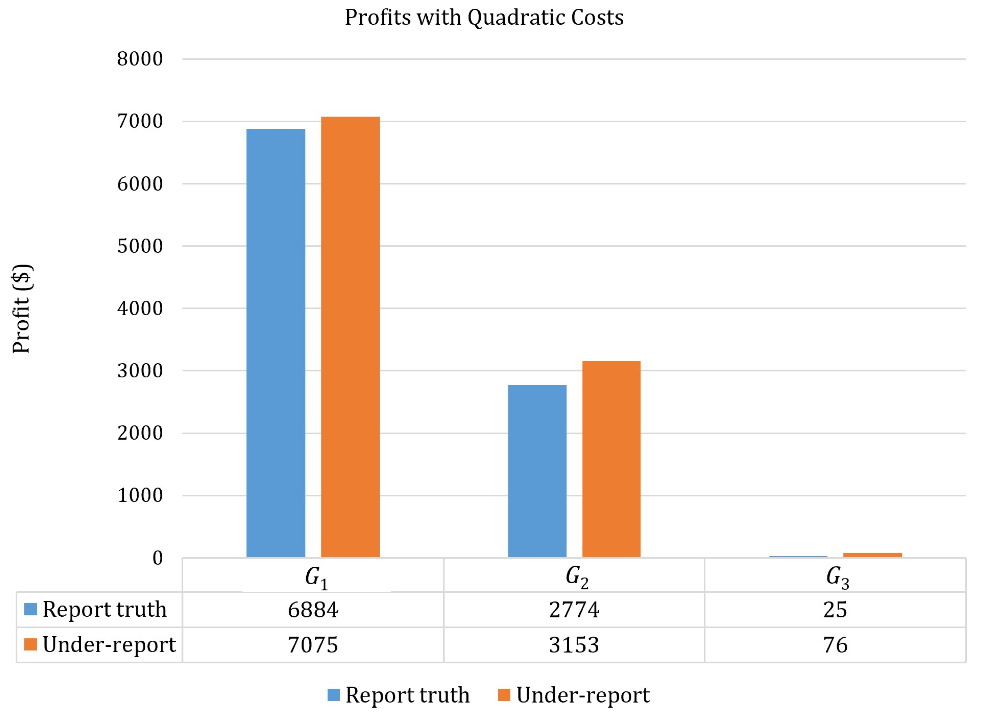
In this subsection, the quadratic cost functions presented in Table 1 are considered. Again, it is assumed that generators and report their true ramp-up and -down rates (the same), and reports their true ramp-up rate (25 MW/h). It is also assumed that may report its ramp-down rate as 25 MW/h (the true value) or 5 MW/h (a low value). The ED and PM problems are solved in the same way described above in Section 3.2. The ED problem is solved twice with the true and low values of the reported down-up rate of . For each scenario, the PM problem is solved with its true ramp rate given the corresponding TLMP for all intervals. Then, the same process is repeated for scenarios where or may not report their true ramp-down value. The results are presented in Table 3 and Figure 5 below. Similar to what is presented in Section 3.2, each generator makes a higher profit by revealing a lower ramp-down rate. This implies that revealing ramping rates truthfully may not be in the best interest of the generators when their costs are quadratic under the TLMP pricing scheme.
In summary, when the generation costs are linear, TLMP is incentive compatible with respect to ramp-rate reporting, and the generator profits are not affected [11]. However, when the generation costs are piecewise linear or quadratic, TLMP is not incentive compatible. A generator might be able to make higher profits by under-reporting its ramp-down rate. This under-reporting of ramp-down rates could result in the possible infeasibility of ED. This may affect the reliability, stability, and overall performance of the grid, leading to operational difficulties within power systems.
4. Conclusions
This paper discusses the incentive compatibility of TLMP with respect to ramp-rate reporting through numerical examples following [11], where it was shown that generators have the incentive to reveal their ramp rates truthfully when the marginal costs of generators are linear. As the linear costs used in [11] are not practical in the current electricity markets, piecewise linear and quadratic costs are considered. In addition, it is assumed that a generator may report different values for its ramp-up and -down rates. The results show that a generator can achieve higher profit by under-reporting its ramp-down rate while reporting its true ramp-up rate when costs are either piecewise linear or quadratic. It is implied that revealing the ramp rate truthfully may not be beneficial for a generator under the TLMP pricing scheme, resulting in the possible infeasibility of ED. This may affect the reliability, stability, and overall performance of the grid, leading to operational difficulties within power systems.
Author Contributions
Conceptualization, F.H., B.Y., P.L., J.Z., F.Z., D.S. and T.Z.; methodology, F.H., B.Y., P.L. and M.B.; software, F.H. and B.Y.; validation, F.H., B.Y., P.L. and M.B.; data curation, F.H.; supervision, T.Z., F.Z., P.L., M.B. and B.Y.; project administration, B.Y. and T.Z.; writing—original draft preparation, F.H., B.Y., P.L. and M.B.; writing—review and editing, F.H., B.Y., P.L., M.B., J.Z., F.Z., D.S. and T.Z.; visualization, F.H. All authors have read and agreed to the published version of the manuscript.
Funding
This work was supported in part by the National Science Foundation under Grants ECCS-1810108, and by a project funded by ISO New England. Any opinions, findings, conclusions or recommendations expressed in this paper are those of the authors and do not reflect the views of NSF or ISO New England.
Data Availability Statement
Data sharing not applicable.
Conflicts of Interest
The authors declare that they have no known competing financial interests or personal relationships that could have appeared to influence the work reported in this paper.
References
- New York Independent System Operator, Inc. Market Administration and Control Area Services Tariff. 2022. Available online: https://nyisoviewer.etariff.biz/ViewerDocLibrary/MasterTariffs/9FullTariffNYISOMST.pdf (accessed on 21 April 2023).
- Corporation, C.I.S.O. California Independent System Operator Corporation Fifth Replacement. 2019. FERC electric tariff. Available online: http://www.caiso.com/Documents/Conformed-Tariff-asof-Sept28-2019.pdf (accessed on 21 April 2023).
- Tong, J.; Ni, H. Look-ahead multi-time frame generator control and dispatch method in PJM real time operations. In Proceedings of the 2011 IEEE Power and Energy Society General Meeting, Detroit, MI, USA, 24–29 July 2011; p. 1. [Google Scholar]
- Hogan, W.W. Electricity market design and zero-marginal cost generation. Curr. Sustain./Renew. Energy Rep. 2022, 9, 15–26. [Google Scholar] [CrossRef]
- Hogan, W.W. Electricity market design: Optimization and market equilibrium. In Proceedings of the Workshop on Optimization and Equilibrium in Energy Economics, Institute for Pure and Applied Mathematics, Los Angeles, CA, USA, 13 January 2016. [Google Scholar]
- Hua, B.; Schiro, D.A.; Zheng, T.; Baldick, R.; Litvinov, E. Pricing in multi-interval real-time markets. IEEE Trans. Power Syst. 2019, 34, 2696–2705. [Google Scholar] [CrossRef]
- Schiro, D.A. Flexibility procurement and reimbursement: A multi-period pricing approach. In Proceedings of the FERC Technical Conference, Washington, DC, USA, 26 June 2017. [Google Scholar]
- Zhao, J.; Zheng, T.; Litvinov, E. A multi-period market design for markets with intertemporal constraints. IEEE Trans. Power Syst. 2019, 35, 3015–3025. [Google Scholar] [CrossRef] [Green Version]
- Yang, Z.; Wang, Y.; Yu, J.; Yang, Y. On the minimization of uplift payments for multi-period dispatch. IEEE Trans. Power Syst. 2020, 35, 2479–2482. [Google Scholar] [CrossRef]
- Guo, Y.; Chen, C.; Tong, L. Pricing multi-interval dispatch under uncertainty part I: Dispatch-following incentives. IEEE Trans. Power Syst. 2021, 36, 3865–3877. [Google Scholar] [CrossRef]
- Chen, C.; Guo, Y.; Tong, L. Pricing multi-interval dispatch under uncertainty part II: Generalization and performance. IEEE Trans. Power Syst. 2020, 36, 3878–3886. [Google Scholar] [CrossRef]
Figure 1.
Generator profits with piecewise linear costs.

Figure 2.
Demand and TLMP of under different reported ramp-down rates.
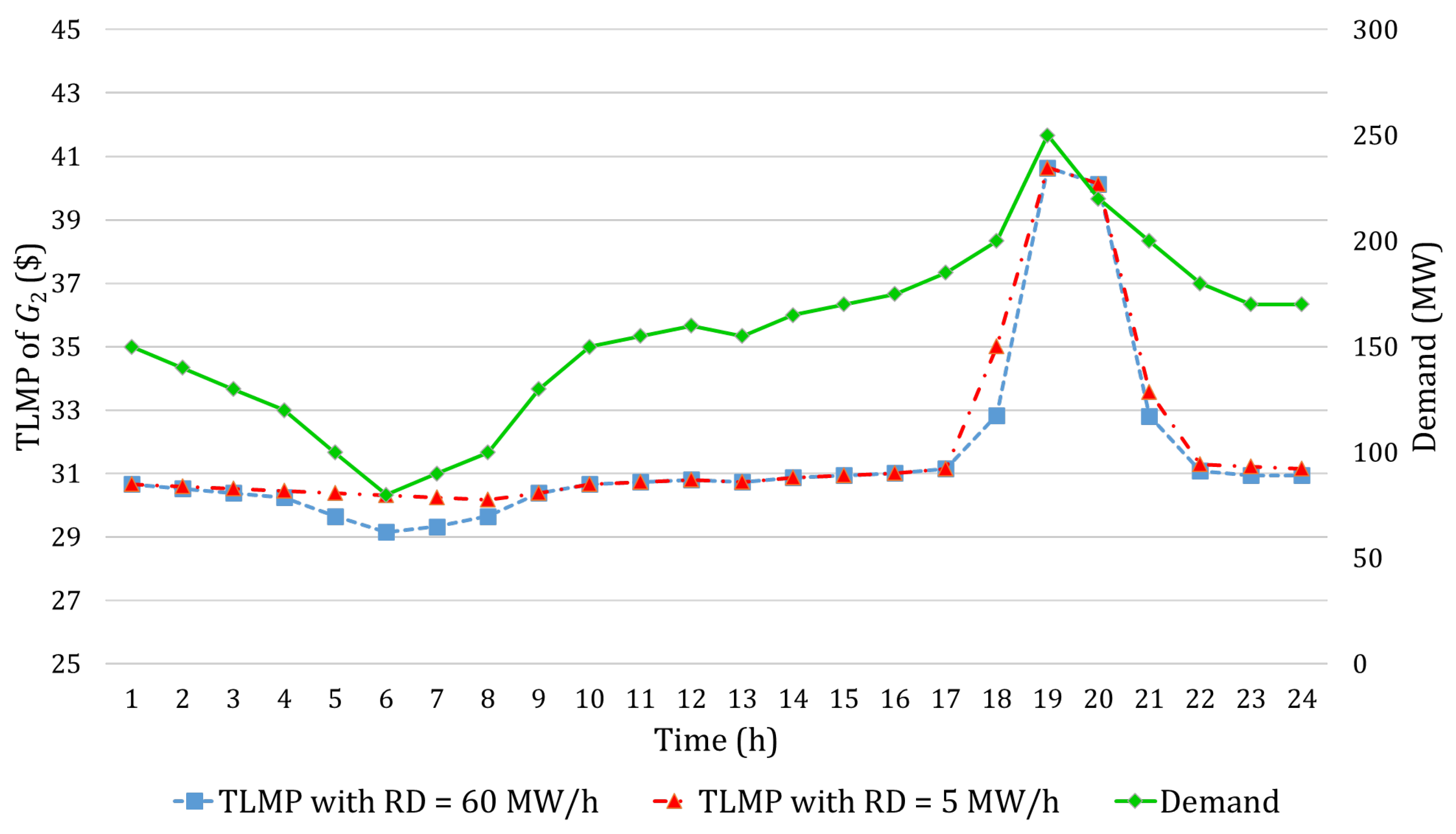
Figure 3.
Demand and power output of under different reported ramp-down rates.
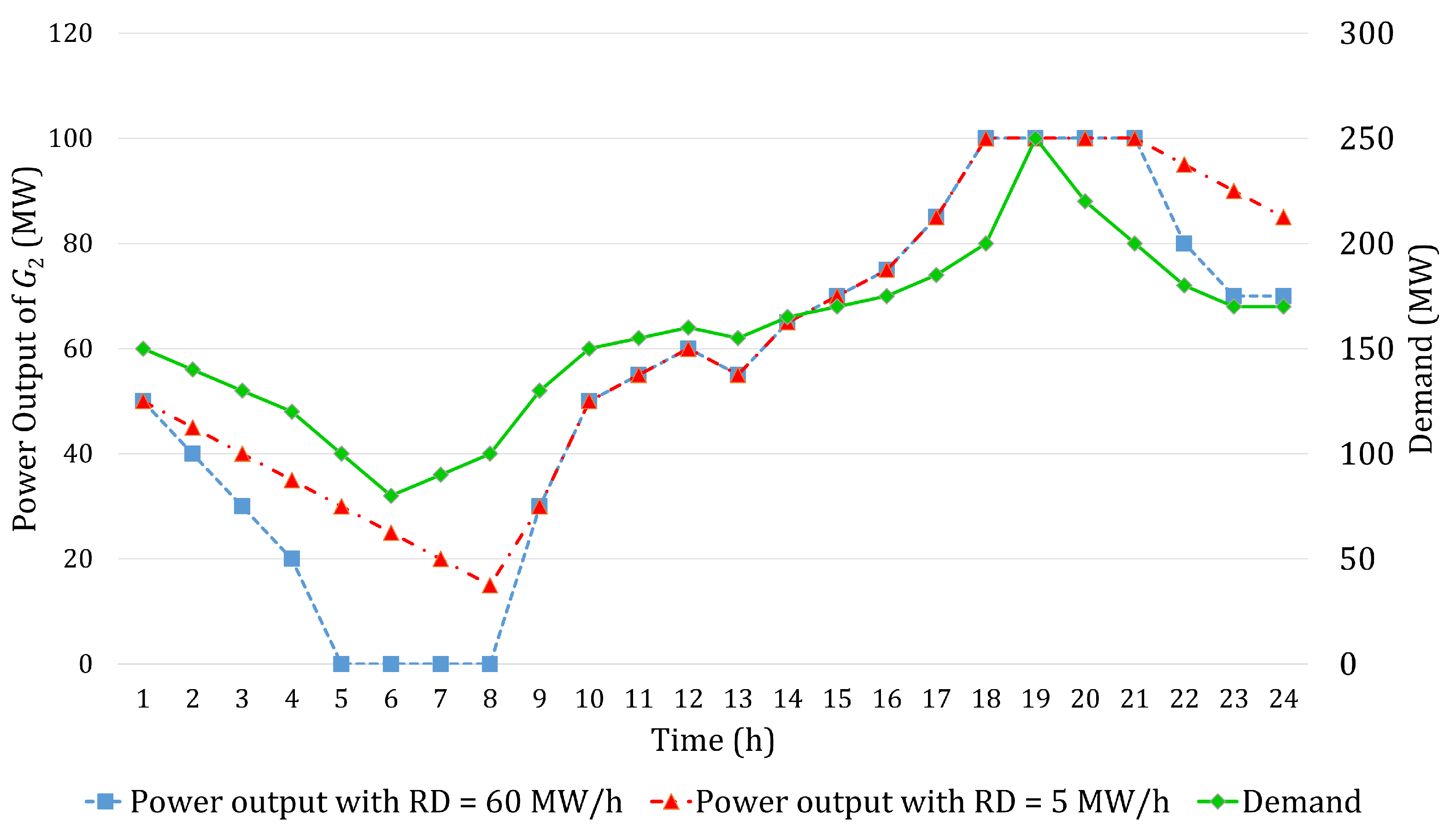
Figure 4.
Demand and profits of under different reported ramp-down rates.
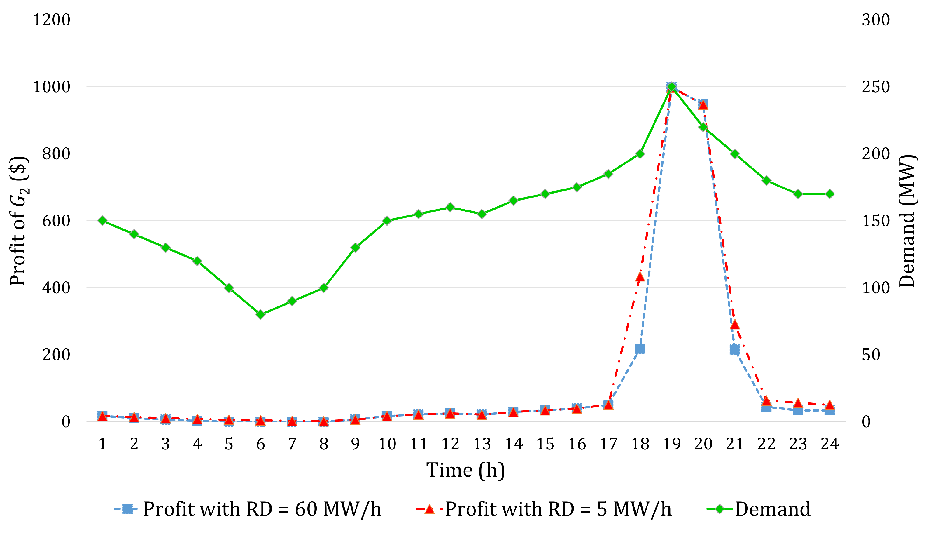
Figure 5.
Generator profits with quadratic costs.

Table 1.
Generator parameters.
| G | Capacity (MW) | True Ramp Rate (MW/h) | Linear Costs ($/MW) | Piecewise Linear Costs ($/MW) | Quadratic Cost Functions ($) |
|---|---|---|---|---|---|
| 100 | 25 | 28 | (28,29) | 0.008568 + 28.7897g | |
| 100 | 60 | 30 | (30,31) | 0.007 + 29.9626g | |
| 100 | 60 | 40 | (40,41) | 0.008568 + 39.7897g |
Table 2.
Profits with piecewise linear costs.
| G | Report Truth | Under-Report | ||
|---|---|---|---|---|
| RD (MW/h) | Profit ($) | RD (MW/h) | Profit ($) | |
| 25 | 7460 | 5 | 8260 | |
| 60 | 3340 | 5 | 3420 | |
| 60 | 0 | 5 | 120 | |
Table 3.
Profits with quadratic costs.
| G | Report Truth | Under-Report | ||
|---|---|---|---|---|
| RD (MW/h) | Profit ($) | RD (MW/h) | Profit ($) | |
| 25 | 6884 | 5 | 7075 | |
| 60 | 2774 | 5 | 3153 | |
| 60 | 25 | 5 | 76 | |
Disclaimer/Publisher’s Note: The statements, opinions and data contained in all publications are solely those of the individual author(s) and contributor(s) and not of MDPI and/or the editor(s). MDPI and/or the editor(s) disclaim responsibility for any injury to people or property resulting from any ideas, methods, instructions or products referred to in the content. |
© 2023 by the authors. Licensee MDPI, Basel, Switzerland. This article is an open access article distributed under the terms and conditions of the Creative Commons Attribution (CC BY) license (https://creativecommons.org/licenses/by/4.0/).
Share and Cite
MDPI and ACS Style
Hyder, F.; Yan, B.; Luh, P.; Bragin, M.; Zhao, J.; Zhao, F.; Schiro, D.; Zheng, T. Discussion on Incentive Compatibility of Multi-Period Temporal Locational Marginal Pricing. Energies 2023, 16, 4977. https://doi.org/10.3390/en16134977
AMA Style
Hyder F, Yan B, Luh P, Bragin M, Zhao J, Zhao F, Schiro D, Zheng T. Discussion on Incentive Compatibility of Multi-Period Temporal Locational Marginal Pricing. Energies. 2023; 16(13):4977. https://doi.org/10.3390/en16134977
Chicago/Turabian StyleHyder, Farhan, Bing Yan, Peter Luh, Mikhail Bragin, Jinye Zhao, Feng Zhao, Dane Schiro, and Tongxin Zheng. 2023. "Discussion on Incentive Compatibility of Multi-Period Temporal Locational Marginal Pricing" Energies 16, no. 13: 4977. https://doi.org/10.3390/en16134977
Note that from the first issue of 2016, this journal uses article numbers instead of page numbers. See further details here.