

Optimal Participation of Co-Located Wind–Battery Plants in Sequential Electricity Markets


Department of Wind and Energy Systems, Risø Campus, Technical University of Denmark (DTU), 4000 Roskilde, Denmark
*
Authors to whom correspondence should be addressed.
Energies 2023, 16(15), 5597; https://doi.org/10.3390/en16155597
Submission received: 21 June 2023
/
Revised: 7 July 2023
/
Accepted: 20 July 2023
/
Published: 25 July 2023
(This article belongs to the Special Issue Advanced Research on Clean Energy and Electricity Market)
Abstract
:Since hybrid power plants (HPPs) play an intensive role in the energy supply balance of future energy systems, there is today increased attention on co-located wind–battery HPPs both in industry and academia. This paper proposes an energy management system (EMS) methodology for wind–battery plants participating in two sequential electricity markets, namely in the spot market (SM) and the balancing market (BM). The proposed and implemented EMS consists of day-ahead (DA) spot market optimization, hour-ahead (HA) balancing market optimization, and intra-hour re-dispatch optimization to allow HPPs to achieve energy arbitrage, to offer regulation power at the HA stage, and to reduce real-time imbalances. The optimization models used in the EMS incorporate an accurate battery degradation model and grid connection constraints. This paper presents a detailed case analysis of the profitability of HPPs in markets towards 2030 based on the proposed EMS. Furthermore, the value of intra-hour re-dispatch optimization in improving the feasibility of generation plans, as well as the impacts of overplanting on wind energy curtailment and battery degradation, is also investigated based on the proposed EMS.
1. Introduction
The green transition of the energy system is witnessing an increase in the share of wind energy [1]. Nevertheless, the power system imbalances caused by the variability and uncertainty of wind generation bring huge challenges to power system operators [2,3]. Such power systems with a large share of wind energy require large power capacity reserves or a huge curtailment of wind power to maintain the power system balance. In this respect, energy storage technologies are seen as potential solutions to mitigate such concerns. These storage technologies can either be connected directly in the power systems close to loads or together with wind power plants (WPPs), forming hybrid power plants (HPPs). Figure 1 illustrates an example diagram of a wind–battery HPP. Compared with a virtual power plant, an obvious feature of the HPP is the co-location; namely, the assets in the HPP share the same point of interconnection. On the one hand, this makes it possible to overplant HPPs with respect to grid connection capacity. Overplanting means increasing the HPP capacity above the grid connection capacity. As an example, a utility-scale HPP—Kennedy Energy Park [4]—was constructed in Queensland, Australia, in 2019. In this project, 12 wind turbines amounting to a 43 MW installed capacity are coupled with 15 MW of solar photovoltaic (PV) and a 2 MW/4 MWh battery energy storage system (BESS). The total installed capacity is higher than the grid connection capacity (50 MW) [4]. It is foreseeable that overplanting helps optimize transmission system utilization and delays the reinforcement of transmission infrastructures during renewable energy integration. On the other hand, an HPP with storage can increase generation flexibility because, by shifting energy through charging or discharging the battery, more stable power can be inserted into the electrical grid [5,6]. This helps the HPP to capture more revenue streams [7] in electricity markets to overcome operation costs including battery degradation costs, etc. One market opportunity is, for example, the balancing market, where HPPs might receive payments by voluntarily providing a balancing service. Individual WPPs are less likely to provide balancing services due to their power variability and uncertainty.
There have been various investigations in the literature regarding the short-term optimal offering challenges of wind–battery HPPs in electricity markets. Comparisons of existing works regarding different aspects are summarized in Table 1. It is clear that all the works cover the aspect of day-ahead (DA) energy trading in the spot market. Additionally, ref. [8] also studies the optimal offering of regulation power in the hour-ahead (HA) balancing market. The grid connection constraint is considered in [9,10], where the total power output of HPPs is limited by the grid connection capacity. However, the models proposed in [9,10] do not include a battery degradation model, which could have significant impacts on the making of generation plans. Ref. [11] proposes a distributionally robust chance-constraint model for the optimal operation of the wind–battery plant in the day-ahead market. The battery degradation is modeled by the battery energy throughput multiplied by the fixed degradation coefficient. The price maker model for wind–battery plants in the day-ahead market is proposed in [12], where the battery degradation cost depends on the depth of discharge (DoD) of the discharging cycles. The degradation in [13,14] is modeled based on the degradation state of the charge curve, while the non-linear relationship between degradation and the DoD is considered in [15]. The others consider neither grid connection constraints nor battery degradation.
Accordingly, none of the aforementioned studies consider both battery degradation and grid connection constraints, which play important roles in the operation of wind–battery plants. Moreover, transmission system operators in many countries have legal or contractual requirements for power plants to track their generation plans. None of the aforementioned studies investigate whether wind–battery plants with variable and uncertain wind generation can track their generation plans.
To fill this gap, this article proposes a novel EMS methodology consisting of three optimization models for wind–battery plants to participate in the spot market and balancing market, including battery degradation and grid connection constraints.
The main contributions of this paper are as follows:
- A novel EMS methodology is proposed for operating wind–battery HPPs in electricity markets considering the battery degradation model and grid connection constraints. The novelty lies in the fact that there has been no method in the literature that considers operation in sequential markets, i.e., the spot market, the balancing market, and real-time operation, as well as the non-linear battery degradation model and grid connection constraints, simultaneously.
- The value of wind–battery HPPs providing regulation power, i.e., a balancing service in the Nordic balancing market in 2030, is investigated by comparing the annual profits of different operation strategies. This value quantification provides HPP developers and owners with knowledge of profit maximization from the balancing market while taking in cognizance the bulk-power offer in the spot market and limiting the overdegradation of batteries.
- The value of intra-hour re-dispatch optimization on improving the feasibility of the generation plan is analyzed through specific case studies. This is particularly relevant as numerous countries have legal or contractual obligations for power plants to adhere to their generation plans.
- A detailed investigation of the impacts of overplanting on wind energy curtailment and battery degradation is performed, which helps HPP developers and owners to understand the potential benefits or adverse effects of overplanting with respect to the grid connection constraints.
2. Methodology
This section discusses the methodology of the developed EMS. As demonstrated in Figure 2, the EMS is on top of the power management system (PMS) (also often referred to as the HPP controller (HPPC) [23]). It works through three optimizations, including DA spot market optimization (SMOpt), HA balancing market optimization (BMOpt), and intra-hour re-dispatch optimization (RDOpt). All optimization models integrate a detailed battery degradation model [24]. The inputs of the EMS are external forecasts of wind power and market prices, updated real-time (RT) information from the PMS, and information from markets and transmission system operators (TSOs). The outputs of the EMS are traded energy and power into markets and energy set-points to the PMS.
2.1. Battery Degradation Model
In this paper, a semi-empirical model (SEM) [24] is used to estimate the loss of capacity (LoC) of the battery. The formulations are given by the following:
Equation (1) provides the non-linear models (as shown in Figure 2) to be used to express the accumulated LoC d for a fresh battery and used battery after the formation of an SEI film, respectively. A pre-defined value , e.g., 8% [24], is used to switch between the models. and are the LoC and linear degradation rate when d exceeds for the first time. The remaining energy capacity is estimated by Equation (2), where is the rated energy capacity of the battery.
The linear degradation rate l in Equation (1), calculated by Equations (3) and (4), depends on the DoD , the elapsed time , the state of charge (SoC) , and the cell temperature .
For each cycle i, the linear degradation rate is calculated by Equation (4), which consists of the cycling degradation and calendar degradation. These two components depend on four stress factor models, including the DoD stress model , time stress model , SoC stress model , and temperature stress model . Their formulations are given as follows [24]:
where , , , , , and are parameters fitted by experiment data. and are the reference SoC and reference temperature, respectively.
It should be noticed that the model is a post-processing model. A rainflow counting [25,26] needs to be implemented on the historical SoC profile to obtain the cycle DoD, cycle average SoC, cycle number, and cycle time duration, as shown in Figure 2. Therefore, the model as it is in this form cannot be directly integrated into optimization.
To solve this problem, a throughput-based model is used to approximate the semi-empirical model based on the assumption that the battery degrades linearly in a short period, e.g., one week. Based on this, the accumulated LoC per MWh throughput, i.e., slope , can be calculated in a short period using the following:
where is the LoC obtained by (1). represents the energy throughput for a past period. Then, the LoC caused by the charging/discharging throughput in a future period can be estimated using the following:
where is the energy throughput for a future period.
2.2. Spot Market Optimization
The goal of spot market optimization is to decide how much energy should be committed to the spot market based on wind power forecasts and spot market price forecasts. This model operates once a day, before the closure of the spot market.
2.2.1. Objective Function
The objective function in the spot market optimization is to maximize profits, i.e., revenues minus the degradation cost, in the spot market, namely,
where , , and are spot price forecasts, the power of the HPP in the SM, and the power of the battery in the SM, respectively. The first item is the revenues from selling energy in the spot market. is typically one hour. represents battery degradation costs given by the following:
where is the marginal degradation cost of the battery. and are the discharging and charging power of the battery in the SM, respectively.
2.2.2. Technical and Operation Constraints
The technical and operation constraints are given as:
where , , , /, , and are the dispatched wind power in the SM, rated power capacity of the battery, stored energy of the battery, minimum/maximum stored energy of the battery, grid connection capacity, and DA wind power forecasts, respectively. Equation (13) calculates the power output of HPPs based on wind and battery generation, where is calculated in (14). Constraints (15) and (16) limit the battery that cannot charge or discharge at the same time, where means the battery works on the discharging status; otherwise, means the battery works on the charging status. Equation (17) models the evolution of battery energy over time. Constraint (18) sets the limits of energy. Constraint (19) details that the power output of HPPs cannot exceed grid limitations. Constraint (20) restricts the wind power output to less than the forecasting value.
2.3. Balancing Market Optimization
The goal of BMOpt is to optimize regulation power offers and update power schedules based on the updated forecast information, e.g., the HA wind power forecast. This model operates hourly, starting from the current OI to the end of the day.
2.3.1. Objective Function
The objective function of BMOpt is to maximize profits in the balancing market, namely,
where , /, /, and / are the HA battery power schedule, upward/downward balancing power offer, positive/negative imbalance power, and charging/discharging power of the battery, respectively. The objective function (21) includes revenues from the regulation power and imbalance settlement, as well as penalties of battery degradation. Revenues from the regulation power and imbalance settlement are computed in (22) and (23), respectively, where and are up and down balancing prices, respectively. They are calculated by and . The represents forecasts of the regulation price (RP) during period k. It should be noticed that the cleared spot prices (SPs) for all days are known in balancing market optimization. and indicate the activation signal of regulation power of the coming hour generated by (25) and (26), which can be regarded as forecasts of the activation signal. refers to the penalties of battery degradation, given in (24), where is the penalty coefficient, which reflects the degradation mode. is the DI, which is typically of a 5-min resolution. is the SI, which is typically an hourly or 15-min resolution. The set is defined as . There is . Therefore, the optimization horizon decreases as time increases.
2.3.2. Technical and Operation Constraints
In BMOpt, a sub-hourly resolution is applied because the TSO requires a higher-resolution power schedule to balance the power system, namely, for ,
where , , and are the HA dispatched wind power, HA plan of stored energy in the battery, and HA wind power forecasts. The constraints in balancing market optimization are defined in a similar way as for spot market optimization, with just the small difference that in balancing market optimization a sub-hourly resolution is applied according to the requirement from the TSO.
2.3.3. Imbalance Settlement Constraints
The revenue from imbalance settlement should also be considered when optimizing regulation power offers and power schedules. This refers to whether HPPs should deliberately create an imbalance in order to capture revenue opportunities from providing regulation power. For , the imbalance settlement constraints are expressed in (35)–(37).
where is the imbalance power in an SI. Equation (35) calculates imbalance power that is the difference between the HA power schedule and DA promised power as well as the regulation power. It is noted that the upward and downward regulating power offer of the current hour, denoted as and , are fixed at the time of executing BMOpt. The set is defined as . There is . The set is defined as .
and are the activation signals of the regulation power of the current hour coming from the TSO. A value of 1 means activation and a value of 0 means no activation.
2.4. Re-Dispatch Optimization
The RDOpt operates between two BMOpts when part of the imbalances has been realized. It repeats every 5 min, which is a nearly real-time optimization starting from the dispatch interval (DI) to the end of the day. The goal of this model is to update the power schedule continuously with real-time information to maximize profits in imbalance settlement and also consider the potential profit opportunities for providing regulation power in future offering intervals (OIs).
2.4.1. Objective Function
The objective function is given as:
The objective function of RDOpt is similar to BMOpt, but the difference is that the index of regulation revenues is , meaning that the start interval for regulation power offers is after 2 OIs because regulation power offers for the current OI and next OI are already determined at the time of optimization. means rounding down.
2.4.2. Technical and Operation Constraints
For , The general constraints are the same as BMOpt, i.e., (27)–(34).
2.4.3. Imbalance Settlement Constraints
In the re-dispatch stage, the calculation of imbalance power is classified into four situations: the current settlement interval (SI), the remaining SIs in the current OI, the SIs in the next OI, and the SIs for the rest of the day. For , the constraints are shown in (36), (37), and (39)–(42):
2.5. Post-Calculation of Revenue and Cost
The profits calculation happens after the operation day when all information is realized. Accordingly, the profits can be calculated. The realized spot market revenue is calculated by multiplying the energy schedule with cleared spot prices:
The realized regulation revenue is equal to activated regulation powers multiplied by RPs (44).
where is the activated regulation power calculated by (45):
The realized imbalance revenue is equal to differences among the real-time measurements and spot market power schedule as well as the activated regulation power multiplied by the up price or down price according to the sign of the delta (46).
where and are the realized imbalance power given in (47) and (48).
where is the real-time measured generation provided by the PMS.
Apart from revenues, the realized battery degradation cost is also calculated in (50) to reflect where the battery lifetime is.
where represents the total number of 100% DOD cycles that make the battery reach a 80% state of health (SoH). is the capital cost of the battery. is the equivalent 100% DoD cycle number, which can be identified by Equations (1), (3), and (4) assuming the observed LoC is loaded by repeated cycles with a 100% DoD and 50% average SoC.
2.6. Real-Time Measurements
In the real world, communication between the EMS and PMS is required to exchange information. The interface of the EMS and PMS is shown in Figure 3 [27], where the EMS provides energy set-points to the PMS and obtains real-time measurement values, e.g., , from the PMS. However, it is impossible to connect the developed EMS to a real PMS to implement long-term case analysis. To solve this problem, a real-time algorithm to emulate active power control logic [23] is proposed as depicted in Figure 4.
In each DI, the behavior of the controller depends on the difference between the available wind power and power reference, battery charging/discharging abilities, and whether the point of connection (PoC) is congested. The final outputs of the algorithm are 3 states with a priority that follows reference > create imbalance > power curtailment.
3. Case Studies
A set of case studies is carried out to assess the performance of the proposed EMS methodology for HPPs in sequential electricity markets and to understand the profitability of HPPs in sequential electricity markets towards the year 2030. As an HPP located in Western Denmark is considered, the market rules of DK1 are applied, where the DI, SI, and OI are 5 min, 15 min, and 1 h, respectively. As shown in Table 2, four operation strategies are considered in the analysis. It should be noted that, since there is no trade of regulation power when using SMOpt and RDOpt, the variables and objective function terms regarding regulation power in RDOpt are not considered. The parameters for the HPP, based on [27] and the Danish Energy Agency catalogue [28], are depicted in Table 3.
All three optimization models proposed and described in the previous section are solved using the solver of IBM Decision Optimisation Studio CPLEX through the docplex python library [29] operating on the DTU’s high-performance computing cluster Sophia [30].
3.1. Wind and Market Data
Wind power time series are simulated with the CorRES simulation tool [31,32,33]. This tool is based on re-analyzing meteorological data from the weather research and forecast model with the stochastic model to add fluctuations. CorRES is capable of simulating wind power time series in minute resolution. The longitude, latitude, and hub height of the HPP, power curves of wind turbines, and simulation period are required as inputs for CoRES to simulate wind power time series. The weather year used for the time series corresponds to 2012. The assumption behind this is that the climate in 2030 does not change compared to 2012. The DA and HA wind power time series forecasts are also obtained from CorRES with the same setup. The 5-min-ahead forecasts are generated based on the realized wind power of the previous 5 min as the forecast of the next 5 min.
The balancing tool chain (BTC) [34] is used to model the SP and RP in 2030 electricity markets, which combines the Balmorel open-source energy system model [35] to emulate the operation of electricity markets from day-ahead to real-time dynamics. This model considers not only Denmark but also neighboring countries. On top of it, an investment optimization of northern central Europe is implemented to have the 2030 energy system scenario [36,37,38]. To simulate wind and solar power time series in the BTC, CorRES is applied to incorporate the correlation between solar and wind, resulting in simulated prices that are correlated with renewable energy generation. Furthermore, the correlation between the renewable energy generation and load is also considered in the BTC. To obtain the SP and RP forecasts, different techniques are used. Specifically, the SP forecast is derived using a long short-term memory network [39]. The RP forecast is obtained via persistence forecast, which simply uses the previous day’s realized price as the forecast of the current day’s price.
Figure 5 shows the DA, HA, and 5-min-ahead forecasts and measurements of wind power as well as the actual and forecasted spot and regulation price. It is noted that the wind power forecasts of the HPP may not be correlated with market prices. For example, the actual wind power during 8 August to 10 August is higher than DA wind power forecasts. However, the regulating price is higher than the spot price; namely, the whole system requires more generation. Therefore, the wind power forecasting errors in this period do not impact the regulating price.
3.2. Annual Profit of HPP
In DK1, deviations between participants’ metering power and most recent power schedules are penalized via a special power imbalance settlement. The settlement is based on the original energy notification, the most recently updated power schedule converting to 15 min resolution time series, and real-time metering power converting to 15 min resolution time series. In every 15 min, deviations bigger than 10 MW are punished. The details of the calculation can be found in [40]. This part of the penalties is also considered to analyze the profitability, which is marked as “special imbalance costs” in Table 4. Accordingly, the annual statistics of revenues and costs for different operation strategies are shown in Table 4 and Figure 6.
As observed in Table 4 and Figure 6, it is clear that the total profit of HPP in the operation strategy SM + BM + RD is the biggest (13.7 M EUR), followed by the operation strategies SM + BM (13.6 M EUR) and SM+RD (12.2 M EUR), respectively, with the lowest profit being achieved in the operation strategy SM (10.3 M EUR). Furthermore, it is also seen that the intra-hour re-dispatch can unilaterally improve the profits of HPP by reducing imbalance costs from 3.9 M EUR to 1.8 M EUR. while providing balancing service can individually improve the profits of THE HPP by capturing the regulation revenue stream leading to almost no penalties in the BM. The comparison illustrates that the profit potential of providing balancing services is higher than the real-time imbalance cost reduction. Moreover, it can also be noticed that the battery degradation cost approximately doubles with the operation strategy SM + BM compared with the operation strategy SM. The reason is the fact that the battery is more stressed when providing a balancing service. However, the aid of intra-hour re-dispatch helps the battery degradation cost decrease by comparing operation strategies SM + BM + RD and SM+BM, which illustrates that energy set-points derived from re-dispatch optimization stress the battery less.
3.3. Value of Re-Dispatch Optimization
In some Nordic countries, there are contractual or legal requirements with regard to participants tracking their most recent generation plans [41]. Due to the fact that wind forecasting errors are relatively smaller as the time is close to real-time, this section verifies the value of intra-hour re-dispatch for obtaining more trackable generation plans.
As shown in Figure 7, one week is picked up randomly to compare the real-time measured power and power schedules for all operation strategies and to analyze whether power schedules are well tracked. Table 5 demonstrates the percentage of time during the year in terms of the exceedance of the 10 MW threshold with different operation strategies. It is clear in Figure 7 that the HPP can follow its power schedule for more time with re-dispatch optimization in (b) and (d) compared with (a) and (c). Moreover, the percentages of exceedance are significantly reduced, from 19% to 0% and from 2% to 0%, respectively, with the implementation of intra-hour re-dispatch optimization in the EMS, as indicated in Table 5. Accordingly, the special imbalance costs are also reduced to zero, as shown in Table 4. Therefore, the energy set-points obtained by intra-hour re-dispatch are easy to track via the PMS. The reason is that a 5 min ahead forecast of wind power is more accurate and hence stresses the battery less when following such power set-points.
3.4. The Impacts of Overplanting on Wind Energy Curtailment
This section investigates the impact of overplanting on wind energy curtailment, which is the ratio between the annual curtailed wind energy and annual available wind energy. We keep the grid connection capacity fixed at 100 MW and vary the wind power plant capacity from 100 MW to 150 MW. The power capacity of the battery changes from 10 MW to 50 MW with a fixed C-rate of . The simulation results are demonstrated in Figure 8.
It is evident that augmenting the capacity of wind power plants leads to a substantial increase in wind energy curtailment, due to the restricted grid connection capacity. For instance, the curtailment percentage rises to when the wind power plant capacity reaches 150 MW, with the minimum battery capacity. Additionally, the figure indicates that increasing the battery size can alleviate the curtailment to some extent, but the wind power plant capacity still dominates the curtailment due to the limited energy capacity of the battery.
3.5. The Impacts of Overplanting on Battery Degradation
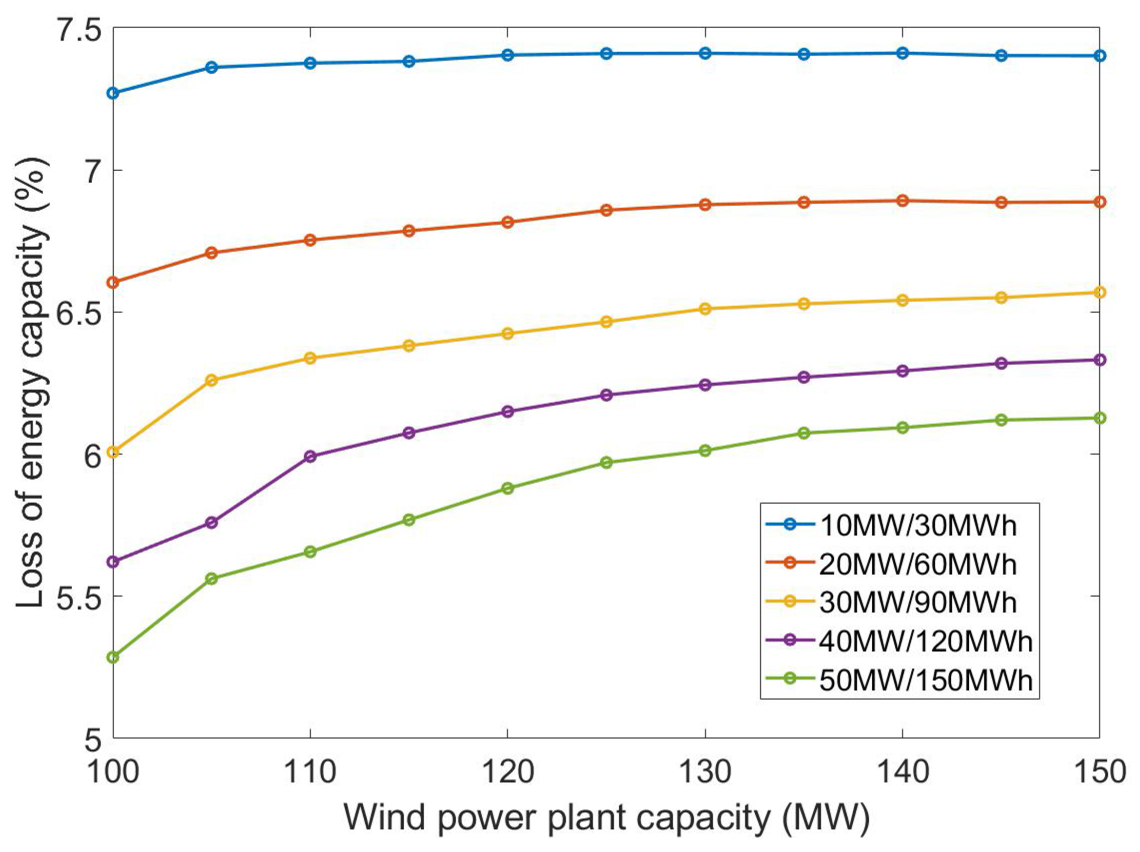
Furthermore, the impacts of overplanting HPPs on battery degradation are also studied with the same HPP configurations. The simulation results are shown in Figure 9.
The figure demonstrates that, irrespective of the battery size, an increase in the wind power plant capacity results in an observable upward trend in the loss of energy capacity. This phenomenon arises due to the deployment of batteries to handle surplus power when the wind power exceeds the grid connection capacity. Additionally, Figure 9 exhibits that the loss of energy capacity curve for relatively smaller batteries plateaus when the wind power plant capacity surpasses a particular value, e.g., 120 MW for a 10 MW/30 MWh battery. This is due to the excess wind power being too substantial for the battery to accommodate. As a result, the battery has already reached its maximum potential and cannot undergo any further degradation.
4. Conclusions
This article has proposed an EMS for wind–battery hybrid power plants (HPPs) in electricity markets, which allows HPPs to obtain revenues from energy arbitrage, the provision of balancing services, and a reduction in real-time imbalances. An annual simulation of wind–battery HPPs in sequential electricity markets towards 2030 has been carried out to analyze the performance of the EMS. The analysis revealed that the balancing market offers profit potential in 2030, with a 33% increase in annual profits compared to participation in the spot market alone. Additionally, the proposed intra-hour re-dispatch optimization helps to formulate more tractable generation plans. The percentages of imbalance power exceeding the 10 MW threshold are reduced to 0% with the intra-hour re-dispatch optimization. However, it was observed that overplanting wind–battery HPPs beyond the grid connection capacity could result in significant wind energy curtailment, which was up to 9% in the studied case. Furthermore, overplanting can also accelerate battery degradation, highlighting the need for the careful planning of wind–battery HPPs to ensure their optimal operation in electricity markets.
This work mainly focused on the EMS methodology for different markets and its application in investigating balancing market potentials. The decisions made by the EMS depend on forecasts. The future work will focus on investigating the impact of forecast errors on the profitability of HPPs and take the uncertainties of the wind power and market prices into account. Moreover, this work assumes the HPP is the price taker. Future work will also focus on the price maker model for the energy management of HPPs.
Author Contributions
Conceptualization, methodology, validation, visualization, and writing—original draft preparation, R.Z.; writing—review and editing, R.Z., K.D. and A.D.H.; supervision, project administration, and funding acquisition, K.D., P.E.S. and A.D.H. All authors have read and agreed to the published version of the manuscript.
Funding
The research performed for this paper received funding from the European Union’s Horizon 2020 research and innovation programme under Marie Skłodowska-Curie grant agreement No. 861398. Kaushik Das would like to thank the funding from EUDP IEA Wind Task 50-Hybrid Power Plants for his contribution.
Data Availability Statement
Not applicable.
Acknowledgments
The authors would like to thank Matti Koivisto, Polyneikis Kanellas, Juan Gea-Bermudez, and Juan Pablo Murcia from the Department of Wind and Energy Systems at Technical University of Denmark for their support for CorRES, the balancing tool chain, and the HPC cluster.
Conflicts of Interest
The authors declare no conflict of interest.
Abbreviations
The following abbreviations are used in this manuscript:
| HPP | Hybrid power plant |
| EMS | Energy management system |
| SM | Spot market |
| BM | Balancing market |
| DA | Day-ahead |
| HA | Hour-ahead |
| WPP | Wind power plant |
| PV | Photovoltaic |
| BESS | Battery energy storage system |
| DoD | Depth of discharge |
| SMOpt | Spot market optimization |
| BMOpt | Balancing market optimization |
| RDOpt | Re-dispatch optimization |
| DI | Dispatch interval |
| SI | Settlement interval |
| OI | Offering interval |
| PMS | Power management system |
| HPPC | Hybrid power plant controller |
| RT | Real time |
| TSO | Transmission system operator |
| SEM | Semi-empirical model |
| LoC | Loss of capacity |
| SoC | State of charge |
| SoH | State of health |
| CorRES | Correlated renewable energy source simulation tool |
| BTC | Balancing tool chain |
| PoC | Point of connection |
References
- Agency, I.E. Renewables 2021-Analysis and forecast to 2026; Technical Report; International Energy Agency: Paris, France, 2021.
- Das, K.; Gea-Bermudez, J.; Kanellas, P.; Koivisto, M.; Leon, J.P.M.; Sørensen, P.E. Recommendations for balancing requirements for future North Sea countries towards 2050. In Proceedings of the 19th Wind Integration Workshop 2020, Online, 11–12 November 2020; Energynautics GmbH: Darmstadt, Germany, 2020. [Google Scholar]
- Shen, J.; Cheng, C.; Jia, Z.; Zhang, Y.; Lv, Q.; Cai, H.; Wang, B.; Xie, M. Impacts, challenges and suggestions of the electricity market for hydro-dominated power systems in China. Renew. Energy 2022, 187, 743–759. [Google Scholar] [CrossRef]
- Petersen, L.; Hesselbæk, B.; Martinez, A.; Borsotti-Andruszkiewicz, R.M.; Tarnowski, G.C.; Steggel, N.; Osmond, D. Vestas power plant solutions integrating wind, solar pv and energy storage. In Proceedings of the 3rd International Hybrid Power Systems Workshop, Tenerife, Spain, 8–9 May 2018; Energynautics: Darmstadt, Germany. [Google Scholar]
- Dykes, K.; King, J.; DiOrio, N.; King, R.; Gevorgian, V.; Corbus, D.; Blair, N.; Anderson, K.; Stark, G.; Turchi, C.; et al. Opportunities for Research and Development of Hybrid Power Plants; National Renewable Energy Laboratory (NREL): Golden, CO, USA, 2020.
- WindEurope. Renewable Hybrid Power Plants: Exploring the Benefits and Market Opportunities; WindEurope: Brussels, Belgium, 2019. [Google Scholar]
- Gorman, W.; Mills, A.; Bolinger, M.; Wiser, R.; Singhal, N.G.; Ela, E.; O’Shaughnessy, E. Motivations and options for deploying hybrid generator-plus-battery projects within the bulk power system. Electr. J. 2020, 33, 106739. [Google Scholar] [CrossRef]
- Wang, Y.; Zhao, H.; Li, P. Optimal offering and operating strategies for Wind-Storage system participating in spot electricity markets with progressive stochastic-robust hybrid optimization model series. Math. Probl. Eng. 2019, 2019, 2142050. [Google Scholar] [CrossRef] [Green Version]
- Ding, H.; Pinson, P.; Hu, Z.; Song, Y. Optimal offering and operating strategies for wind-storage systems with linear decision rules. IEEE Trans. Power Syst. 2016, 31, 4755–4764. [Google Scholar] [CrossRef] [Green Version]
- Das, K.; Grapperon, A.L.T.P.; Sørensen, P.E.; Hansen, A.D. Optimal battery operation for revenue maximization of wind-storage hybrid power plant. Electr. Power Syst. Res. 2020, 189, 106631. [Google Scholar] [CrossRef]
- Xu, X.; Hu, W.; Cao, D.; Huang, Q.; Liu, Z.; Liu, W.; Chen, Z.; Blaabjerg, F. Scheduling of wind-battery hybrid system in the electricity market using distributionally robust optimization. Renew. Energy 2020, 156, 47–56. [Google Scholar] [CrossRef]
- Mohamed, M.A.; Jin, T.; Su, W. An effective stochastic framework for smart coordinated operation of wind park and energy storage unit. Appl. Energy 2020, 272, 115228. [Google Scholar] [CrossRef]
- Loukatou, A.; Johnson, P.; Howell, S.; Duck, P. Optimal valuation of wind energy projects co-located with battery storage. Appl. Energy 2021, 283, 116247. [Google Scholar] [CrossRef]
- Wang, Y.; Zhou, Z.; Botterud, A.; Zhang, K.; Ding, Q. Stochastic coordinated operation of wind and battery energy storage system considering battery degradation. J. Mod. Power Syst. Clean Energy 2016, 4, 581–592. [Google Scholar] [CrossRef] [Green Version]
- Khaloie, H.; Anvari-Moghaddam, A.; Contreras, J.; Toubeau, J.F.; Siano, P.; Vallée, F. Offering and bidding for a wind producer paired with battery and CAES units considering battery degradation. Int. J. Electr. Power Energy Syst. 2022, 136, 107685. [Google Scholar] [CrossRef]
- Ding, H.; Pinson, P.; Hu, Z.; Song, Y. Integrated bidding and operating strategies for wind-storage systems. IEEE Trans. Sustain. Energy 2015, 7, 163–172. [Google Scholar] [CrossRef] [Green Version]
- Cai, Z.; Bussar, C.; Stöcker, P.; Moraes, L., Jr.; Magnor, D.; Sauer, D.U. Optimal dispatch scheduling of a wind-battery-system in German power market. Energy Procedia 2016, 99, 137–146. [Google Scholar] [CrossRef]
- Crespo-Vazquez, J.L.; Carrillo, C.; Diaz-Dorado, E.; Martinez-Lorenzo, J.A.; Noor-E-Alam, M. A machine learning based stochastic optimization framework for a wind and storage power plant participating in energy pool market. Appl. Energy 2018, 232, 341–357. [Google Scholar] [CrossRef]
- Al-Lawati, R.A.; Crespo-Vazquez, J.L.; Faiz, T.I.; Fang, X.; Noor-E-Alam, M. Two-stage stochastic optimization frameworks to aid in decision-making under uncertainty for variable resource generators participating in a sequential energy market. Appl. Energy 2021, 292, 116882. [Google Scholar] [CrossRef]
- Abdeltawab, H.H.; Mohamed, Y.A.R.I. Market-oriented energy management of a hybrid wind-battery energy storage system via model predictive control with constraint optimizer. IEEE Trans. Ind. Electron. 2015, 62, 6658–6670. [Google Scholar] [CrossRef]
- Han, X.; Hug, G. A distributionally robust bidding strategy for a wind-storage aggregator. Electr. Power Syst. Res. 2020, 189, 106745. [Google Scholar] [CrossRef]
- Crespo-Vazquez, J.L.; Carrillo, C.; Diaz-Dorado, E.; Martinez-Lorenzo, J.A.; Noor-E-Alam, M. Evaluation of a data driven stochastic approach to optimize the participation of a wind and storage power plant in day-ahead and reserve markets. Energy 2018, 156, 278–291. [Google Scholar] [CrossRef]
- Long, Q.; Das, K.; Pombo, D.V.; Sørensen, P.E. Hierarchical control architecture of co-located hybrid power plants. Int. J. Electr. Power Energy Syst. 2022, 143, 108407. [Google Scholar] [CrossRef]
- Xu, B.; Oudalov, A.; Ulbig, A.; Andersson, G.; Kirschen, D.S. Modeling of lithium-ion battery degradation for cell life assessment. IEEE Trans. Smart Grid 2016, 9, 1131–1140. [Google Scholar] [CrossRef]
- Downing, S.D.; Socie, D. Simple rainflow counting algorithms. Int. J. Fatigue 1982, 4, 31–40. [Google Scholar] [CrossRef]
- Shi, Y.; Xu, B.; Tan, Y.; Zhang, B. A convex cycle-based degradation model for battery energy storage planning and operation. In Proceedings of the 2018 Annual American Control Conference (ACC), Milwaukee, WI, USA, 27–29 June 2018; IEEE: Piscataway, NJ, USA, 2018; pp. 4590–4596. [Google Scholar]
- Long, Q.; Zhu, R.; Das, K.; Sørensen, P.E. Interfacing Energy Management with Supervisory Control for Hybrid Power Plants. In Proceedings of the 20th Wind Integration Workshop 2021, Hybrid Conference, Berlin, Germany, 29–30 September 2021. [Google Scholar]
- Agency, D.E. Technology Data for Energy Storage. Available online: https://ens.dk/sites/ens.dk/files/Analyser/technology_data_catalogue_for_energy_storage.pdf (accessed on 25 November 2021).
- IBM. Decision Optimization Modeling for Python (DOcplex). Available online: https://github.com/IBMDecisionOptimization/docplex-doc (accessed on 25 November 2021).
- Technical University of Denmark. Sophia HPC Cluster. In Research Computing at DTU. 2019. Available online: https://dtu-sophia.github.io/docs/ (accessed on 25 November 2021). [CrossRef]
- Murcia Leon, J.P.; Koivisto, M.J.; Sørensen, P.; Magnant, P. Power fluctuations in high-installation-density offshore wind fleets. Wind. Energy Sci. 2021, 6, 461–476. [Google Scholar] [CrossRef]
- Koivisto, M.; Das, K.; Guo, F.; Sørensen, P.; Nuño, E.; Cutululis, N.; Maule, P. Using time series simulation tools for assessing the effects of variable renewable energy generation on power and energy systems. Wiley Interdiscip. Rev. Energy Environ. 2019, 8, e329. [Google Scholar] [CrossRef]
- Koivisto, M.; Jónsdóttir, G.M.; Sørensen, P.; Plakas, K.; Cutululis, N. Combination of meteorological reanalysis data and stochastic simulation for modelling wind generation variability. Renew. Energy 2020, 159, 991–999. [Google Scholar] [CrossRef]
- Kanellas, P.; Das, K.; Gea-Bermudez, J.; Sørensen, P. Balancing Tool Chain: Balancing and Automatic Control in North Sea Countries in 2020, 2030 and 2050; DTU Wind Energy: Roskilde, Denmark, 2020. [Google Scholar]
- Wiese, F.; Bramstoft, R.; Koduvere, H.; Alonso, A.P.; Balyk, O.; Kirkerud, J.G.; Tveten, Å.G.; Bolkesjø, T.F.; Münster, M.; Ravn, H. Balmorel open source energy system model. Energy Strategy Rev. 2018, 20, 26–34. [Google Scholar] [CrossRef]
- Koivisto, M.; Gea-Bermúdez, J.; Sørensen, P. North Sea offshore grid development: Combined optimisation of grid and generation investments towards 2050. IET Renew. Power Gener. 2020, 14, 1259–1267. [Google Scholar] [CrossRef] [Green Version]
- Gea-Bermúdez, J.; Pade, L.L.; Koivisto, M.J.; Ravn, H. Optimal generation and transmission development of the North Sea region: Impact of grid architecture and planning horizon. Energy 2020, 191, 116512. [Google Scholar] [CrossRef]
- Gea-Bermúdez, J.; Jensen, I.G.; Münster, M.; Koivisto, M.; Kirkerud, J.G.; Chen, Y.k.; Ravn, H. The role of sector coupling in the green transition: A least-cost energy system development in Northern-central Europe towards 2050. Appl. Energy 2021, 289, 116685. [Google Scholar] [CrossRef]
- Hochreiter, S.; Schmidhuber, J. Long short-term memory. Neural Comput. 1997, 9, 1735–1780. [Google Scholar] [CrossRef] [PubMed]
- Energinet. Regulation C2: The Balancing Market and Balance Settlement 2023. Available online: https://energinet.dk/media/pufj5pkx/forskrift-c2.pdf (accessed on 1 May 2023).
- Model, N.B. Current Requirements for Production Plans and Imbalances, Monitoring and the Use of Production Plans in Balancing. Available online: https://nordicbalancingmodel.net/wp-content/uploads/2020/03/Current-requirements-for-production-plans-and-imbalances_FINAL.pdf (accessed on 25 November 2021).
Figure 1.
Diagram example for a wind–battery hybrid power plant.

Figure 2.
Diagram of energy management system and its interface with other models and agents.

Figure 3.
An overview of HPP EMS and HPP PMS [27].
Figure 3.
An overview of HPP EMS and HPP PMS [27].

Figure 4.
Real-time simulation algorithm.
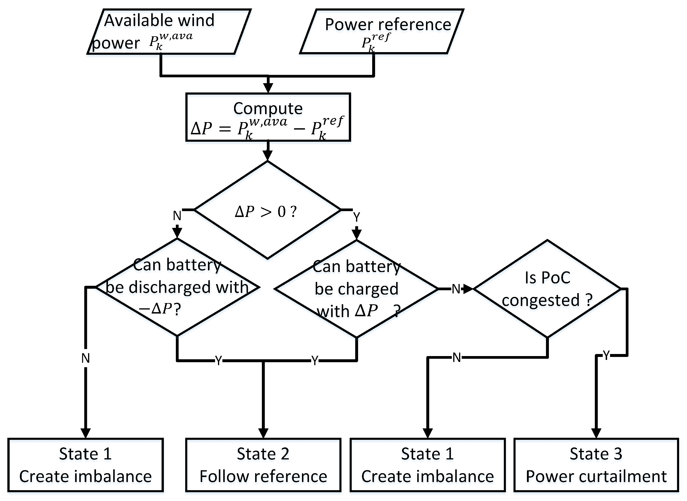
Figure 5.
Demonstration of wind and market data in one week: (a) DA, HA, and 5-min-ahead forecast and measurement of wind power time series; (b) forecasted and actual SP time series; (c) forecasted and actual RP time series.
Figure 5.
Demonstration of wind and market data in one week: (a) DA, HA, and 5-min-ahead forecast and measurement of wind power time series; (b) forecasted and actual SP time series; (c) forecasted and actual RP time series.
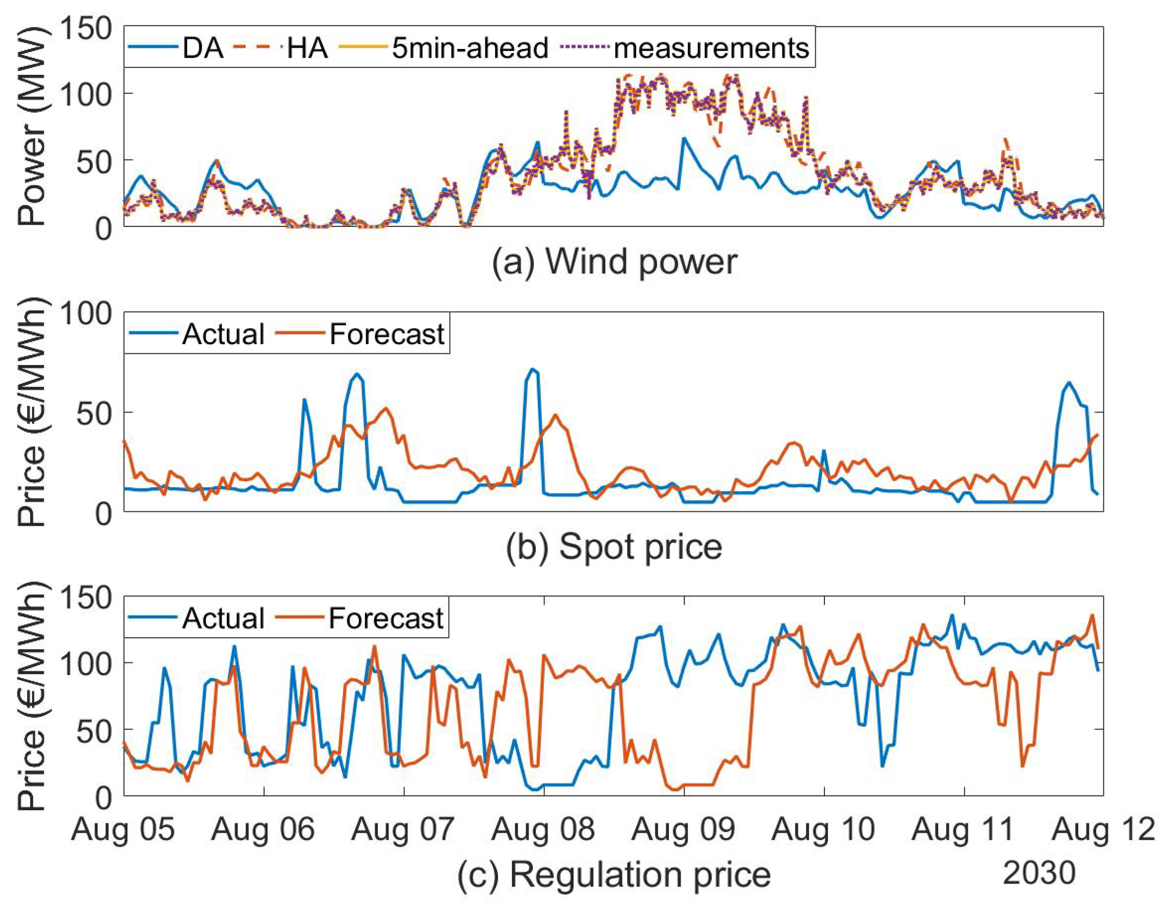
Figure 6.
Comparison of SM revenue, BM revenue, degradation cost, and total profits of all operation strategies.
Figure 6.
Comparison of SM revenue, BM revenue, degradation cost, and total profits of all operation strategies.

Figure 7.
Real-time power measurements and power schedules with different operation strategies: (a) SM; (b) SM + RD; (c) SM+BM; (d) SM + BM + RD.
Figure 7.
Real-time power measurements and power schedules with different operation strategies: (a) SM; (b) SM + RD; (c) SM+BM; (d) SM + BM + RD.

Figure 8.
Wind energy curtailment (%) with different capacities of wind power plants.

Figure 9.
Loss of energy capacity (%) with different capacity of wind power plants.

Table 1.
Overview and comparison of the research focus in the literature and the work presented in this paper.
Table 1.
Overview and comparison of the research focus in the literature and the work presented in this paper.
| Ref. No. | Time Scale | Battery Degradation | Grid Connection Constraints | ||
|---|---|---|---|---|---|
| DA Energy Offering | HA Regulation Power Offering | Intra-Hour Balancing | |||
| [8] | 🗸 | 🗸 | |||
| [9] | 🗸 | 🗸 | |||
| [10] | 🗸 | 🗸 | |||
| [11] | 🗸 | 🗸 | |||
| [12] | 🗸 | 🗸 | |||
| [13] | 🗸 | 🗸 | |||
| [15] | 🗸 | 🗸 | |||
| [14] | 🗸 | 🗸 | |||
| [16] | 🗸 | ||||
| [17] | 🗸 | ||||
| [18] | 🗸 | ||||
| [19] | 🗸 | ||||
| [20] | 🗸 | ||||
| [21] | 🗸 | ||||
| [22] | 🗸 | ||||
| This work | 🗸 | 🗸 | 🗸 | 🗸 | 🗸 |
Table 2.
Operation strategy definition.
| Operation Strategy | Spot Market | Balancing Market | |
|---|---|---|---|
| SMOpt | BMOpt | RDOpt | |
| SM | 🗸 | ||
| SM + RD | 🗸 | 🗸 | |
| SM + BM | 🗸 | 🗸 | |
| SM + BM + RD | 🗸 | 🗸 | 🗸 |
Table 3.
Parameters of the HPP.
| Item | Parameters | Values |
|---|---|---|
| WPP | 120 MW | |
| BESS | 20 MW | |
| 60 MWh | ||
| 12 MWh | ||
| 97% | ||
| 98% | ||
| 0% | ||
| 0.142 M EUR/MWh | ||
| 11.72 M EUR | ||
| Grid | 100 MW |
Table 4.
Annual revenues and costs of HPP with different operation strategies (million EUR).
| Operation Strategy | SM Revenues | BM Revenues | Total Revenues | Degradation Costs | Total Profits | |||
|---|---|---|---|---|---|---|---|---|
| Regulation Revenues | Imbalance Revenues | Special Imbalance Costs | Total | |||||
| SM | 14.7 | 0 | −2.0 | 2.0 | −4.0 | 10.7 | 0.4 | 10.3 |
| SM + RD | 14.5 | 0 | −1.8 | 0.0 | −1.8 | 12.7 | 0.5 | 12.2 |
| SM + BM | 14.6 | 3.9 | −4.1 | 0.1 | −0.3 | 14.3 | 0.7 | 13.6 |
| SM + BM + RD | 14.5 | 4.0 | −4.1 | 0.0 | −0.2 | 14.3 | 0.6 | 13.7 |
Table 5.
Percentage of time during the year that the difference between and exceeds 10 MW threshold with different operation strategies.
Table 5.
Percentage of time during the year that the difference between and exceeds 10 MW threshold with different operation strategies.
| SM | SM + RD | SM + BM | SM + BM + RD | |
|---|---|---|---|---|
| Percentage (%) | 19 | 0 | 2 | 0 |
Disclaimer/Publisher’s Note: The statements, opinions and data contained in all publications are solely those of the individual author(s) and contributor(s) and not of MDPI and/or the editor(s). MDPI and/or the editor(s) disclaim responsibility for any injury to people or property resulting from any ideas, methods, instructions or products referred to in the content. |
© 2023 by the authors. Licensee MDPI, Basel, Switzerland. This article is an open access article distributed under the terms and conditions of the Creative Commons Attribution (CC BY) license (https://creativecommons.org/licenses/by/4.0/).
Share and Cite
MDPI and ACS Style
Zhu, R.; Das, K.; Sørensen, P.E.; Hansen, A.D. Optimal Participation of Co-Located Wind–Battery Plants in Sequential Electricity Markets. Energies 2023, 16, 5597. https://doi.org/10.3390/en16155597
AMA Style
Zhu R, Das K, Sørensen PE, Hansen AD. Optimal Participation of Co-Located Wind–Battery Plants in Sequential Electricity Markets. Energies. 2023; 16(15):5597. https://doi.org/10.3390/en16155597
Chicago/Turabian StyleZhu, Rujie, Kaushik Das, Poul Ejnar Sørensen, and Anca Daniela Hansen. 2023. "Optimal Participation of Co-Located Wind–Battery Plants in Sequential Electricity Markets" Energies 16, no. 15: 5597. https://doi.org/10.3390/en16155597
Note that from the first issue of 2016, this journal uses article numbers instead of page numbers. See further details here.