
Assessment of Converter Performance in Hybrid AC-DC Power System under Optimal Power Flow with Minimum Number of DC Link Control Variables
National Institute of Technology Silchar, Silchar 788010, India
*
Author to whom correspondence should be addressed.
Energies 2023, 16(15), 5800; https://doi.org/10.3390/en16155800
Submission received: 30 June 2023
/
Revised: 25 July 2023
/
Accepted: 28 July 2023
/
Published: 4 August 2023
(This article belongs to the Special Issue Optimization and Control for Power Grid with the Support of HVDC Systems)
Abstract
:This paper presents a strategy to evaluate the performances of converter stations under the optimized operating points of hybrid AC-DC power systems with a reduced number of DC link variables. Compared to previous works reported with five DC-side control variables (CVs), the uniqueness of the presented optimal power flow (OPF) formulation lies within the selection of only two DC-side control variables (CVs), such as the inverter voltage and current in the DC link, apart from the conventional AC-side variables. Previous research has mainly been focused on optimizing hybrid power system performance through OPF-based formulations, but has mostly ignored the associated converter performances. Hence, in this study, converter performance, in terms of ripple and harmonics in DC voltage and AC current and the utilization of the converter infrastructure, is evaluated. The minimization of active power loss is taken as an objective function, and the problem is solved for a modified IEEE 30 bus system using a recently developed and very efficient Archimedes optimization algorithm (AOA). Case studies are performed to assess the efficacy of the presented OPF model in power systems, as well as converter performance. Furthermore, the results are extended to assess the applicability of the proposed model to the allocation of photovoltaic (PV)-type distributed generations (DGs) in hybrid AC-DC systems. The average improvement in power loss is found to be around 7.5% compared to the reported results. Furthermore, an approximate 10% improvement in converter power factor and an approximate 50% reduction in ripple factor are achieved.
1. Introduction
Due to the advancement in solid-state technologies, the applications of power-electronics-based converters in power systems have rapidly increased recently. In particular, high-voltage direct current (HVDC) transmission systems and the integration of power electronics interface-based renewable energy sources (RESs) are the dominant ones [1,2,3]. For example, India’s total HVDC terminal capacity reached to 33,500 MW by the end of 2022 [4], and the percentage of PV-based RES in total installed capacity is around 15% [5]. The key benefits of HVDC systems are the higher-power throughputs [6], flexibility of power flow control [7,8], and ease in submarine power transmission [9,10]. Given the advantages mentioned above, transforming modern power systems from conventional AC systems to hybrid AC-DC systems and increasing the penetration of RES are inevitable trends [11,12]. Hence, the research to establish a framework for the coordinated control and optimization of hybrid power systems with RES is crucial.
However, challenges arise due to the distinct AC and DC system model, wherein HVDC converters are mainly line-commutated converters (LCCs) or voltage-source converters (VSCs) connected through HVDC cables [13,14]. The control of the HVDC link is carried out through constant current, constant ignition angle, constant voltage, constant extinction angle control, etc., and is generally performed by the adjustment of variables, like the tap ratio, firing angle, direct current, and direct voltage [15]. However, the selection of these variables depends on the choice of the control strategy. The optimum values of these variables can be decided based on the operational requirements of a given hybrid AC-DC power system.
Of late, some studies related to the planning and operation of hybrid AC-DC power systems have been reported in the literature [16,17,18,19,20,21,22,23,24,25,26,27,28,29,30]. A survey revealed that the authors had performed the studies through an optimization approach called optimal power flow (OPF). Conceptually, an OPF is a non-convex and nonlinear complex optimization problem that aims to optimize certain objective(s) while obeying all operational constraints (equality and inequality) with the adjustment of control settings (variables) [31]. Generally, the power balance equations in OPF represent the equality constraints and power apparatuses’ operational limits, load bus voltage limits, line flow limits, etc., forming the inequality constraints. The literature further reveals that the OPF problem becomes more complex for hybrid AC-DC power systems because of the addition of CV associated with the HVDC link and the interaction between AC and DC systems [23]. In modeling, a sequential method of load flow is used to tackle the interaction between AC and DC systems [23,24,25,26,27,28,29,30]; in solving the DC system, the AC bus voltages of either end of the DC link are kept constant, and for the AC system, the DC link is modeled with fixed reactive and active power injections. In [17,18,19], the converter reactive and active power injections are added in load flow equations, and the linkage between AC and DC systems is addressed by adding equality constraints associated with converters.
When viewed as an optimization problem, the solution of OPF for hybrid AC-DC systems is very challenging. Authors in the past have applied the sequential gradient-restoration algorithm [16], linear programming [19,20,21], steepest descent algorithm [18], interior point method [17,22], etc., to solve OPF for hybrid AC-DC systems. They have considered voltage deviation [16,17], active power loss [17,18,19,20,22], cost [16,18], and the voltage stability index [21] as objective functions in their work. A survey revealed that the conventional methods stated above are cumbersome with respect to the integration of HVDC modeling in OPF and higher computational requirements [23]. Nevertheless, they do not guarantee optimum solutions for practical nonlinear, non-convex problems. Consequently, researchers have applied metaheuristic approaches [23,24,25,26,27,28,29,30] to solve the complex OPF problem for hybrid AC-DC power systems.
Particularly, in [23], optimal reactive power dispatch (ORPD), considering active power loss minimization as an objective function, was addressed by modifying the existing differential evolution (DE) method with a novel neighborhood mutation step. The applicability of the method was tested by applying it to a large-scale practical power system (Algerian 114 bus). Similarly, in [30], a modification in the DE algorithm using a local search mutation was suggested to overcome the problems of poor exploitation and a local optima trap. The method was tested for the OPF problem with generation cost as an objective function and applied to four hybrid AC-DC power systems. In [25], the ORPD with real power loss as an objective was solved using the genetic algorithm (GA), and a comparative analysis was shown for three different test systems. In [24], by applying the artificial bee colony (ABC) optimization technique, the authors addressed the single-objective OPF problem with the aim of either generation cost or active power loss. Arithmetic crossover was suggested to enhance the performance of the moth swarm algorithm [27]. The superiority of this modified algorithm was verified by applying it to a standard benchmark test system and an OPF problem in a hybrid power system. Three objective functions, namely, the voltage stability index, power generation cost, and voltage deviation, were explored individually on a New England 39 bus system. In [28], the backtracking search algorithm (BSA) was used to solve the hybrid power system’s active power loss minimization problem. Furthermore, the optimal allocation of distributed generation was also explored. Similarly, BSA was also used to solve an optimal generation cost problem for a power system with a two-terminal HVDC link [26]. A comparative analysis for CPU time and objective function value was also provided. In [29], the authors applied the ABC algorithm to solve the loss minimization problem and presented a statistical comparison.
It has been revealed from the state of the art [23,24,25,26,27,28,29,30] that the previous authors consider as many as five CVs per HVDC link. Among these, four are related to reactive and active power injections at the inverter and rectifier stations, and the fifth one is the direct current of the HVDC link. A critical observation reveals that the simultaneous consideration of active power at both the converter stations, along with the direct current as an independent CV, may cause a mismatch at times in the power balance of the HVDC link. Moreover, the converter may operate with wider variations of firing angle. Consequently, to examine the effect of the firing angle on the utilization of the converter infrastructure, power factor, and harmonic injection, further study on converter performance is required. Therefore, the selection of proper variables for HVDC links is an important task and has not been carried out in the past. A summary of the main contributions of this work is highlighted as follows:
- The assessment of HVDC converter performances through a conventional OPF formulation is unique and presented for the first time in the literature.
- Identifying the possibilities of power imbalances in the DC link in the case of random selection of DC-side CVs, such as power at converter stations, DC link current, etc., in the OPF formulation and summarizing its impact on converter performance is novel. Based on the above, an OPF with only two CVs on the DC side is proposed for a hybrid AC-DC system.
- Analyzing the effectiveness of the devised model in converter performances side by side with power system indices can be considered the first of its kind in the literature.
- The assessment of the applicability of the proposed model to the allocation of PV-type DG in hybrid AC-DC systems is a unique contribution to the best of the authors’ knowledge.
When viewed as an optimization problem, the present OPF is very complex and challenging. Of late, the trend of verifying the applicability of new metaheuristics for engineering solutions can be witnessed globally among researchers. Recently, the application of AOA was witnessed to solve OPF for AC systems [32]. The obtained results were promising, giving strong reason to continue the further investigation on verifying the search capability of AOA in order to solve the highly complex optimization problems of hybrid AC-DC systems.
The organization of the paper is as follows: The modeling of the LCC-based two-terminal HVDC link and the derived OPF model for hybrid AC-DC systems are presented in Section 2 and Section 3, respectively. In Section 4, a brief overview of AOA and its implementation for the considered OPF problem is given. The results of case studies on modified IEEE 30 bus systems are shown in Section 5. Comparative analysis and the converter performance evaluation at optimal points are also presented in the same section. Section 6 presents the conclusion of various case studies performed in the paper.
2. Modeling of HVDC
A schematic representation of the two-terminal HVDC link is illustrated in Figure 1. The HVDC link includes a DC line and two converter stations connected at either end of the HVDC line. AC buses at the sending and receiving ends are represented by bus r and bus i, respectively.
The rectifier converter is connected to AC bus r through the converter transformer at one end of the HVDC line. At the other end, the inverter is connected to AC bus i. The voltage at buses r and i are indicated by and , respectively. The tap ratio of converter transformers, connected at both ends of the HVDC line, are represented by and . The direct current flowing through the DC line is indicated by . and represent the DC link voltage at the rectifier and inverter end, respectively.
In Figure 2, based on assumptions pertaining to ripples, losses of transformers and converters mentioned in [25], the equivalent circuit of the LCC based two-terminal HVDC link is shown. The and denote the extinction advance and ignition delay angles for the inverter and rectifier converter, respectively. The maximum no-load DC voltage at inverter and rectifier end are denoted as and , respectively.
With the consideration of equal voltage and power base on both DC and AC sides, the basic equations related to the inverter and rectifier side can be expressed as follows:
Here, and are the reactive and active power injections at the rectifier station and and are the injections at the inverter end. and denote equivalent commutating resistance of the inverter and rectifier converter, respectively, and and are the converter power factor angles seen from the inverter and rectifier end.
The linkage between the inverter and rectifier terminals can be expressed as follows:
3. Background of the Research and Mathematical Formulation
3.1. Control Variables
The following five CVs for the DC link are considered in the work reported in [23,24,25,26,27,28,29,30].
With the given set of CVs, as per Equation (8), certain observations related to the calculation of and DC link resistance, , are made to evolve the present mathematical model. For this, 100 different random combinations of , , and are generated, and the consequences are presented in Figure 3 for a DC link resistance of 0.05 pu.
A careful observation reveals that due to the independent selection of , , and to fulfill the power balance equation, as in Equation (7), the value of needs to be adjusted, as shown in Figure 3. The worst scenario arises when the independent selected value of is greater than , and then, can even take negative values. However, due to being a physical property of the DC link, the value of cannot be adjusted. Moreover, one can use either a power Equation (4) or linkage Equation (6) to calculate . However, ambiguity arises as they provide different values, creating confusion on the selection of the exact firing angles. Furthermore, the independent selection of , , , and may operate converters with wider variations in power factor.
Therefore, unlike the five CVs considered in the literature [23,24,25,26,27,28,29,30], in this work, only two CVs, namely, DC link voltage at the inverter () and dc current (), are chosen as the CV of the DC side (), which overcomes the above-mentioned issues. Reducing CV is beneficial when viewed as an optimization problem, as this leads to a smaller search dimension problem.
However, other CVs related to the AC side are kept the same, as in previous works [23,24,25,26,27,28,29,30]. In this work, real power generation () except the slack bus, the generator voltage (), the tap ratio of transformers (t), and the reactive power output of synchronous condenser or shunt capacitor () are selected as the CV of the AC side ().
where NG, NT, and NC represent the number of generators, transformers, and reactive power compensator devices, respectively.
3.2. State Variable
On the AC side, generally, the slack bus output (), load bus voltage magnitude (), and generator reactive power output () are considered as AC state variables ().
where NP represents the total number of load buses.
However, on the DC-side tap ratio of the converter transformers ( and ), active ( and ) and reactive ( and ) powers at the converter, delay angles (,), and DC link voltage at the rectifier () are considered as state variables ().
3.3. Objective Function
Active power loss: In this paper, due to the utilities’ minimum loss energy dispatch target, the total active power loss (Ploss), including both AC and DC transmission lines, is considered an objective function. Mathematically, this is described as follows:
where NL represents the number of lines, and and are the resistance and current of the line.
3.4. Constraints
3.4.1. Equality Constraints
Figure 4 illustrates the representation of AC bus m with the HVDC link. From the figure, it can be observed that the set of equality constraints in terms of the active and reactive power balance equations can be derived as follows:
where and are the real power generation and active power demand, respectively, at the bus. Similarly, is the reactive power demand wherein and are the reactive power generation from the generator and synchronous condenser or shunt capacitor, respectively.
At the bus, the net active and reactive power injections, and , can be described as follows:
Here, and denote the magnitude and phase angle of voltage at the bus, and can be obtained by extracting the real and imaginary parts of the element (m and n) of the bus admittance matrix (Ybus), and N represents the total number of buses in the system.
It can be noted that in the presence of the HVDC converter at the bus, and represent the active and reactive powers injected from the AC system into the converter.
3.4.2. Inequality Constraints
4. Archimedes Optimization Algorithm
A novel metaheuristic optimization algorithm called AOA was presented by Hashim et al. [33]. The algorithm is inspired from the law of physics named Archimedes’ principle, which emulates a buoyant force experienced by a completely or partly immersed object in the fluid. Like other metaheuristic algorithms, AOA is also a population-based optimization tool wherein the optimization process starts with randomly initializing the objects (population) within the search space. The density and volume of each object are modified based on the best object, while each individual’s acceleration is evaluated based on collisions with neighbors. The AOA algorithm’s detailed steps and pseudo code are presented in [33]. A flowchart of AOA for the considered optimization problem is presented in Figure 5.
5. Simulation Results and Discussion
To demonstrate the efficacy of the presented strategy for the selection of CV, the proposed OPF model is solved using the metaheuristic AOA for modified IEEE 30 bus systems (Appendix A). The modified IEEE 30 bus system data are taken from [28,34]. A description of various case studies performed in this work is given in Table 1.
The programs were developed in MATLAB, version 2020b, on a computer with an Intel Core i5 processor, 1.60 GHz, and 8 GB RAM. The tuning parameters of AOA were properly adjusted before declaring the optimum results. The , , , and values were selected as 2, 6, 2, and 0.5, respectively, in all cases. Again, a population size of 30 and a maximum iteration of 200 were found to be suitable for the case studies. The feasibility results were obtained through a penalty-based approach. The optimized results were declared after 30 trial runs. The search capability of AOA was compared with methods reported in the state-of-the-art literature. To assess the converter performance, various power quality indices (Appendix B) were evaluated based on the results through the proposed OPF and reported OPF with five CVs.
5.1. Result Analysis without Considering DG
In Case 1 and Case 2, the OPF problem is solved to minimize the active power loss for the modified IEEE 30 bus systems. Altogether, 13 CVs are adjusted during the optimization, among which 2 CVs are related to the asynchronous tie. The best results for both cases are presented in Table 2. The optimized values of CV and a few important state variables are also mentioned in Table 2. The shaded portions in Table 2 represent the optimized values of the CV obtained and reported in various research works. It can be observed that under the optimized CV, the minimum power losses obtained with AOA are 11.47 MW and 11.0246 MW for Case 1 and Case 2, respectively. A comparison with other reported methods available in the literature reveals that AOA is able to optimize the real power loss by maximum value among all other methods. Moreover, to verify the feasibility of the obtained solution, the bus voltage magnitudes are plotted in Figure 6, showing that all bus voltages are within their permissible limits [28,29]. Moreover, the parametric analysis to select the tunable parameters is presented in Table 3. As mentioned in [33], 24 different combinations are explored, and the optimum value of power loss for each combination is presented in Table 3. The values of 2, 6, 2, and 0.5 are found to be best for , , , and , respectively.
To assess the converter performance, the converters’ power factor angles, extinction advance angle, and ignition delay angle were analyzed. It is worth noting that the lower values of the above-mentioned angles would ensure better operational aspects of the power system from a reactive power and voltage management point of view. The numerical values of the angles obtained for various methods are mentioned in Table 2 and plotted in Figure 7. It can be observed that the angles obtained through the proposed model are significantly lower than other contemporary methods, as the proposed strategy for CV selection ensures the operation of the converter at the smallest possible firing angle. Furthermore, the operation of the converter at a higher power factor is ensured due to a lower firing angle. For example, in Case 1, the inverter station operates at a power factor of 0.8944 in the case of the previously reported OPF with five CVs, while in the case of the proposed OPF, the power factor is 0.9853.
Furthermore, the harmonic components in the DC link voltage and AC currents were analyzed. The harmonics of the 6th, 12th, and 18th orders in the DC link voltage, as a percentage of the no-load maximum DC voltage, were evaluated for the results obtained through various optimization techniques and are plotted in Figure 8 and Figure 9. For all the orders of harmonics, a significant reduction can be observed in the case of AOA, which results from obtaining a lower value in the ignition delay and extinction advance angle with the proposed minimum CV. Similarly, the reduction factor for the harmonics of the 5th, 7th, 11th, and 13th orders of the AC current was evaluated and is presented in Table 4 and Table 5. The obtained results for AOA are better than BSA [28] and ABC [29], as the overlap angles obtained under the proposed OPF are the highest.
Moreover, the performance parameters, like the valve utilization factor (VUF), form factor (FF) [35], ripple factor (RF) [35], transformer utilization factor (TUF) [35], and total demand distortion (TDD) [36], were also evaluated for the optimal solution from the proposed OPF, as well as from the reported OPF with five CVs. The values obtained for both cases are tabulated in Table 6 and Table 7. A careful observation reveals that in the case of the proposed OPF, the obtained values of FF and RF are lowest among all the methods, indicating the minimum harmonic content in the DC link voltage. Similarly, the lowest value is achieved for VUF, which signifies the better utilization of converter infrastructure. The lowest values of FF, RF, and VUF are the result of the proposed selection of CVs, which ensures the operation of the converter with a lower firing angle. Likewise, the obtained values of TDD for AOA in both cases are slightly better compared to other methods due to higher value of overlap angles.
5.2. Result Analysis Considering DG
This section examines the applicability of the devised model in determining the DG allocation problem in hybrid AC-DC systems. In previous work [28], three numbers of PV-type DGs were considered. Hence, here, in Case 3 and Case 4, the OPF is also solved to find the optimal location and size for three DGs, with the objective of real power loss minimization. In the problem formulation, two inequality constraints for each DG are added, and PV power is the added inequality constraint of the active power Equation (14). The best results obtained by AOA for both cases are tabulated in Table 8. Moreover, the values of all CVs and a few important state variables are presented in Table 8. The shaded portions in Table 8 represent the optimized values of the CV obtained and reported in various research works. The optimal locations of DGs in Case 3 are 5, 19, and 30, and in Case 4, the optimal locations are 5, 24, and 30. Moreover, the optimal size of all DGs is 10 MW by AOA, indicating the highest penetration of DGs. A comparison of the results with the methods reported in the recent literature is presented in Table 8. The best value of 8.5842 MW is obtained for real power loss in Case 3 using AOA, and it is better by 6.99% using BSA [28] and 8.90% using ABC [28]. Similarly, the real power loss in Case 4 is 8.0435 MW, which is the lowest among all the methods. Compared to Cases 1 and 2, it can be observed that a considerable reduction in power loss in Cases 3 and 4 is achieved due to the optimal allocation of DGs. To show the feasibility of the solutions, the voltage magnitude of all buses in both cases is shown in Figure 10.
In order to showcase the effectiveness of the proposed selected CV, the firing angle and power factor angle of the converters were evaluated for the optimal solutions and are presented in Figure 11. All the angles obtained in the case of the proposed OPF are lower compared to other reported methods, which is due to the facility of the proposed strategy to ensure the operation of the converter with the minimum firing angle. Because of the same reason, the converter station operates at a higher power factor. For example, in Case 3, the rectifier and inverter station operate at power factors of 0.9776 and 0.9836, respectively, which are the highest among all the considered methods.
Furthermore, similar to previous cases, the harmonic components in the DC link voltage and AC currents were evaluated for the results obtained through AOA and reported in the literature and are presented in Figure 12 and Figure 13 and Table 9 and Table 10. Due to the assurance of the lower values of the ignition delay and extinction advance angle with the proposed strategy of CV selection, the values for all orders of harmonics in the DC link voltage are minimum in the case of AOA. For example, in Case 3, the 6th, 12th, and 18th harmonics evaluated as a percentage of no-load maximum DC voltage at the rectifier side are 6.4772, 2.6607, and 1.6643, respectively, which are the minimum values among all the methods. Similarly, due to higher value of the overlap angle, the obtained values of all harmonics in the AC current are minimum in the case of AOA.
Moreover, for both cases, the performance parameters, like VUF, FF, RF, TUR, and TDD, were also evaluated and are tabulated in Table 11 and Table 12. Due to obtaining a lower value in the firing angle with the selected CV, the lowest value is achieved for FF, RF, TDD, and VUF. This ensures operation with a lower harmonic content in the DC link voltage and AC current and better utilization of the converter infrastructure. Moreover, the value of TUF is also highest in both the cases, which signifies the better utilization of the converter transformer.
6. Conclusions
This study presented an OPF formulation with objective of active power loss for hybrid AC-DC systems with minimum CV at the DC links. For the first time, in this study, an analysis on the performance of HVDC converter stations under OPF in hybrid AC-DC systems was carried out. The considered OPF was applied to a modified IEEE 30 bus system and solved using AOA. The major findings of the presented work are summarized below:
- With the proposed OPF model, the active power loss (without considering DG) was found to be 4% (8%) better than that reported in the existing literature with BSA (ABC).
- The DC link converter station could operate with 10% improved power factor conditions, as compared to the reported OPF with five CVs. The main reason for this is the ability of the converter stations to operate at lower firing angles. Typically, this is smaller in comparison to the reported results.
- Furthermore, the lower value of the firing angle led to a noteworthy reduction of about 10–30% in VUF. Similarly, in all cases, the obtained value of RF was near about half compared to the methods reported in the literature. Likewise, improvements in other performance parameters, like FF, TUF, and TDD, were also observed with the selected CV.
- The proposed OPF model was also suitable for optimal DG allocation in hybrid power systems. Along with highest DG integration and improved converter performance, a notable reduction of 8% (10%) in active power loss was found compared to the reported results by BSA (ABC).
Author Contributions
Conceptualization, C.P. and T.M.; methodology, C.P. and T.M.; software, C.P.; validation, C.P., T.M. and S.S.; formal analysis, C.P., T.M. and S.S.; writing—original draft preparation, C.P.; writing—review and editing, T.M. and S.S.; supervision, T.M. and S.S. All authors have read and agreed to the published version of the manuscript.
Funding
This research received no external funding.
Data Availability Statement
The references for the data are mentioned in the article.
Conflicts of Interest
The authors declare no conflict of interest.
Abbreviations
The following abbreviations are used in this manuscript:
| OPF | Optimal power flow |
| CV | Control variable |
| HVDC | High-voltage direct current |
| AOA | Archimedes optimization algorithm |
| PV | Photovoltaic |
| DG | Distributed generation |
| RES | Renewable energy source |
| LCC | Line-commutated converter |
| VSC | Voltage-source converter |
| ORPD | Optimal reactive power dispatch |
| DE | Differential evolution |
| GA | Genetic algorithm |
| ABC | Artificial bee colony |
| BSA | Backtracking search algorithm |
| VUF | Valve utilization factor |
| TUF | Transformer utilization factor |
| TDD | Total demand distortion |
| FF | Form factor |
| RF | Ripple factor |
| Voltage magnitude at bus r | |
| Angle of voltage at bus r | |
| Direct current | |
| , | Direct voltage at rectifier and inverter end, respectively |
| , | No-load maximum DC voltage at rectifier and inverter end, respectively |
| DC link resistance | |
| , | Tap ratio at rectifier and inverter, respectively |
| Ignition delay angle | |
| Extinction advance angle | |
| , | Rectifier active and reactive power |
| , | Inverter active and reactive power |
| , | Rectifier and inverter end power factor |
| DC link control variable | |
| AC-side control variable | |
| DC link state variable | |
| AC-side state variable | |
| , | Active and reactive power of generator |
| NG | Number of generators |
| Tap ratio of transformer | |
| NT | Number of transformers |
| Reactive power injection by synchronous condenser | |
| NC | Number of synchronous condensers |
| NP | Number of load buses |
| Active power loss | |
| NL | Number of lines |
| Resistance of line | |
| Current through line | |
| Ybus | Bus admittance matrix |
Appendix A
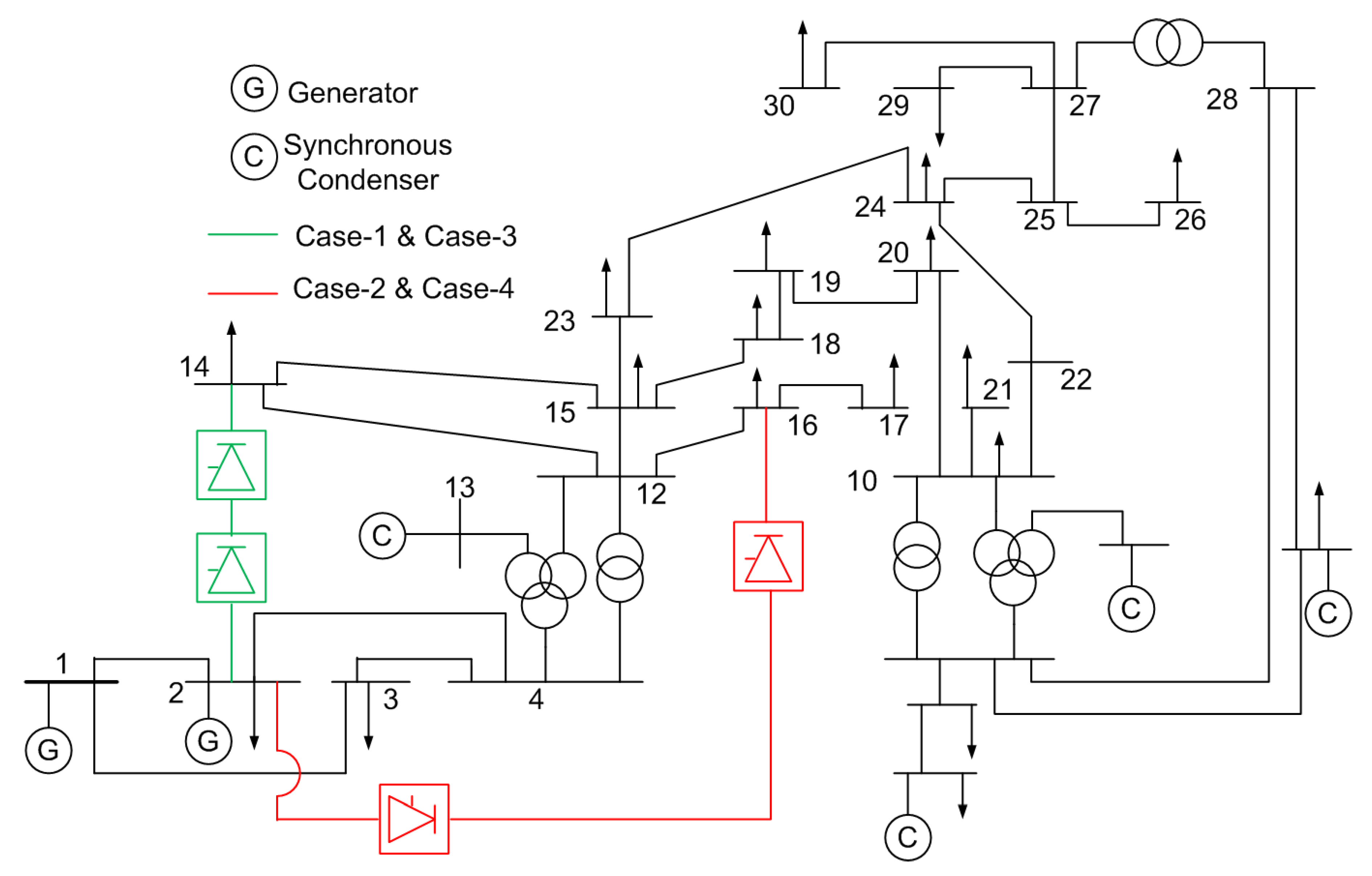
The single-line diagram of modified IEEE 30 bus test system is presented in Figure A1. The two-terminal LCC-based HVDC link is inserted in IEEE 30 bus system to make it a hybrid AC-DC system. Particularly, HVDC link is inserted between bus 2 and bus 14 in Case 1 and Case 3, whereas the link is connected between bus 2 and bus 16 in Case 2 and Case 4.
Figure A1.
Modified IEEE 30 bus test system.
Appendix B
The equations for the performance evaluation of the LCC-based HVDC converter are as follows:
1. Converter power factor
where and are the reactive and active power injection at the converter station, respectively.
2. Form factor (FF)
where and are the rms and average value of voltage.
3. Ripple factor (RF)
where is the dc value of voltage.
4. Total demand distortion (TDD)
where and are the rms values of the fundamental component and total current, respectively, and is the maximum value of current.
5. Transformer utilization ration (TUF)
6. Valve utilization factor (VUF)
where PIV and are the peak inverse voltage of the valve and the direct voltage of the converter, respectively.
7. Reduction factor for harmonics in AC current
where is the harmonic current of order, is the harmonic current of order without the overlap angle, is the firing angle, and is the overlap angle.
8. Harmonics in DC voltage
where is the harmonic voltage of order and is the no-load maximum direct voltage.
References
- Baseer, M.A.; Alsaduni, I. A Novel Renewable Smart Grid Model to Sustain Solar Power Generation. Energies 2023, 16, 4784. [Google Scholar] [CrossRef]
- Huang, X.; Wang, H.; Zhou, Y.; Zhang, X.; Wang, Y.; Xu, H. Photovoltaic Power Plant Collection and Connection to HVDC Grid with High Voltage DC/DC Converter. Electronics 2021, 10, 3098. [Google Scholar] [CrossRef]
- ABB. Special Report—60 Years of HVDC. ABB Group. Available online: https://library.e.abb.com/public/aff841e25d8986b5c1257\d380045703f/140818$%$20ABB$%$20SR$%$2060$%$20years$%$20of$%2$0HVDC_72dpi.pdf (accessed on 1 June 2023).
- “Progress of Substations in the Country”, Central Electricity Authority, Ministry of Power, Government of India. Available online: https://cea.nic.in/wp-content/uploads/transmission/2022/11/GS_SS_1.pdf (accessed on 1 June 2023).
- All India Installed Capacity (in MW) of Power Stations. Central Electricity Authority, Ministry of Power, Government of India. Available online: https://cea.nic.in/wp-content/uploads/installed/2022/11/IC_Nov_2022.pdf (accessed on 1 June 2023).
- Oliveira, D.; Leal, G.C.B.; Herrera, D.; Galván-Díez, E.; Carrasco, J.M.; Aredes, M. An Analysis on the VSC-HVDC Contribution for the Static Voltage Stability Margin and Effective Short Circuit Ratio Enhancement in Hybrid Multi-Infeed HVDC Systems. Energies 2023, 16, 532. [Google Scholar] [CrossRef]
- Wang, Y.; Wu, L.; Chen, S. A Simplified Model of the HVDC Transmission System for Sub-Synchronous Oscillations. Sustainability 2023, 15, 7444. [Google Scholar] [CrossRef]
- Pragati, A.; Mishra, M.; Rout, P.K.; Gadanayak, D.A.; Hasan, S.; Prusty, B.R. A Comprehensive Survey of HVDC Protection System: Fault Analysis, Methodology, Issues, Challenges, and Future Perspective. Energies 2023, 16, 4413. [Google Scholar] [CrossRef]
- Wu, Y.K.; Gau, D.Y.; Tung, T.D. Overview of Various Voltage Control Technologies for Wind Turbines and AC/DC Connection Systems. Energies 2023, 16, 4128. [Google Scholar] [CrossRef]
- Marzinotto, M.; Molfino, P.; Nervi, M. On the Measurement of Fields produced by Sea Return Electrodes for HVDC Transmission. In Proceedings of the 2020 International Symposium on Electromagnetic Compatibility-EMC EUROPE, Rome, Italy, 23–25 September 2020. [Google Scholar]
- Zhou, B.; Ai, X.; Fang, J.; Yao, W.; Zuo, W.; Chen, Z.; Wen, J. Data-adaptive robust unit commitment in the hybrid AC/DC power system. Appl. Energy 2019, 254, 113784. [Google Scholar] [CrossRef]
- Lekić, A.; Ergun, H.; Beerten, J. Initialisation of a hybrid AC/DC power system for harmonic stability analysis using a power flow formulation. High Volt. 2020, 5, 534–542. [Google Scholar] [CrossRef]
- Li, G.; Liang, J.; Joseph, T.; An, T.; Lu, J.; Szechtman, M.; Zhuang, Q. Feasibility and reliability analysis of LCC DC grids and LCC/VSC hybrid DC grids. IEEE Access 2019, 7, 22445–22456. [Google Scholar] [CrossRef]
- Battaglia, A.; Buono, L.; Marzinotto, M.; Palone, F.; Patti, S. LCC and beyond: The new SaCoI link. In Proceedings of the 2021 AEIT HVDC International Conference (AEIT HVDC), Genoa, Italy, 27–28 May 2021. [Google Scholar]
- Kundur, P.B. Power System Stability and Control, 1st ed.; McGraw Hill Education: Noida, India, 2006. [Google Scholar]
- de Martinis, U.; Gagliardi, F.; Losi, A.; Mangoni, V.; Rossi, F. Optimal load flow for electrical power systems with multiterminal HVDC links. IEE Proc. (Gener. Transm. Distrib.) 1990, 137, 139–145. [Google Scholar] [CrossRef]
- Li, Q.; Liu, M.; Liu, H. Piecewise normalized normal constraint method applied to minimization of voltage deviation and active power loss in an AC–DC hybrid power system. IEEE Trans. Power Syst. 2014, 30, 1243–1251. [Google Scholar] [CrossRef]
- Arifoglu, U.; Tarkan, N. New sequential AC-DC load-flow approach utilizing optimization techniques. Eur. Trans. Electr. Power 1999, 9, 93–100. [Google Scholar] [CrossRef]
- Sreejaya, P.; Iyer, S.R. Optimal reactive power flow control for voltage profile improvement in AC-DC power systems. In Proceedings of the 2010 Joint International Conference on Power Electronics, Drives and Energy Systems & 2010 Power India, New Delhi, India, 20–23 December 2010. [Google Scholar]
- Taghavi, R.; Seifi, A. Optimal reactive power control in hybrid power systems. Electr. Power Components Syst. 2012, 40, 741–758. [Google Scholar] [CrossRef]
- Thukaram, D.; Yesuratnam, G. Optimal reactive power dispatch in a large power system with AC–DC and FACTS controllers. IET Gener. Transm. Distrib. 2008, 2, 71–81. [Google Scholar] [CrossRef]
- Yu, J.; Yan, W.; Li, W.; Wen, L. Quadratic models of AC–DC power flow and optimal reactive power flow with HVDC and UPFC controls. Electr. Power Syst. Res. 2008, 78, 302–310. [Google Scholar] [CrossRef]
- Sayah, S. Modified differential evolution approach for practical optimal reactive power dispatch of hybrid AC–DC power systems. Appl. Soft Comput. 2018, 73, 591–606. [Google Scholar] [CrossRef]
- Kılıç, U.; Ayan, K. Optimizing power flow of AC–DC power systems using artificial bee colony algorithm. Int. J. Electr. Power Energy Syst. 2013, 53, 592–602. [Google Scholar] [CrossRef]
- Kılıç, U.; Ayan, K.; Arifoğlu, U. Optimizing reactive power flow of HVDC systems using genetic algorithm. Int. J. Electr. Power Energy Syst. 2014, 55, 1–12. [Google Scholar] [CrossRef]
- Ayan, K.; Kılıç, U. Optimal power flow of two-terminal HVDC systems using backtracking search algorithm. Int. J. Electr. Power Energy Syst. 2016, 78, 326–335. [Google Scholar] [CrossRef]
- Duman, S. A modified moth swarm algorithm based on an arithmetic crossover for constrained optimization and optimal power flow problems. IEEE Access 2018, 6, 45394–45416. [Google Scholar] [CrossRef]
- Fadel, W.; Kilic, U.; Ayan, K. Optimal reactive power flow of power systems with two-terminal HVDC and multi distributed generations using backtracking search algorithm. Int. J. Electr. Power Energy Syst. 2021, 127, 106667. [Google Scholar] [CrossRef]
- KILIÇ, U.; Ayan, K. Artificial bee colony algorithm based optimal reactive power flow of two-terminal HVDC systems. Turk. J. Electr. Eng. Comput. Sci. 2016, 24, 1075–1090. [Google Scholar] [CrossRef]
- Sayah, S.; Hamouda, A. Optimal power flow solution of integrated AC-DC power system using enhanced differential evolution algorithm. Int. Trans. Electr. Energy Syst. 2019, 29, e2737. [Google Scholar] [CrossRef]
- Sahay, S.; Upputuri, R.; Kumar, N. Optimal power flow-based approach for grid dispatch problems through Rao algorithms. J. Eng. Res. 2023, 11, 100032. [Google Scholar] [CrossRef]
- Akdag, O. A improved Archimedes optimization algorithm for multi/single-objective optimal power flow. Electr. Power Syst. Res. 2022, 206, 107796. [Google Scholar] [CrossRef]
- Hashim, F.A.; Hussain, K.; Houssein, E.H.; Mabrouk, M.S.; Al-Atabany, W. Walid Archimedes optimization algorithm: A new metaheuristic algorithm for solving optimization problems. Appl. Intell. 2021, 51, 1531–1551. [Google Scholar] [CrossRef]
- The IEEE 30-Bus Test System. Available online: https://labs.ece.uw.edu/pstca/pf30/ieee30cdf.txt (accessed on 10 March 2023).
- Rashid, M.H. Power Electronics: Devices, Circuits, and Applications, 4th ed.; Pearson Education: Chennai, India, 2017. [Google Scholar]
- Abdalla, O.H.; Elmasry, S.; El Korfolly, M.I.; Htita, I. Harmonic Analysis of an Arc Furnace Load Based on the IEEE 519-2014 Standard. In Proceedings of the 2022 23rd International Middle East Power Systems Conference (MEPCON), Cairo, Egypt, 13–15 December 2022. [Google Scholar]
Figure 1.
A schematic representation of a two-terminal HVDC link.

Figure 2.
An equivalent circuit of a two-terminal HVDC link.

Figure 3.
Combinations of CV and associated and .

Figure 4.
A representation of AC bus m connected to HVDC link.

Figure 5.
Flowchart of AOA for OPF for hybrid AC-DC system.

Figure 6.
Voltage profiles for Case 1 and Case 2.

Figure 7.
Comparison of , , , and for Case 1 and Case 2.

Figure 8.
Harmonics in DC voltages in Case 1.

Figure 9.
Harmonics in DC voltages in Case 2.
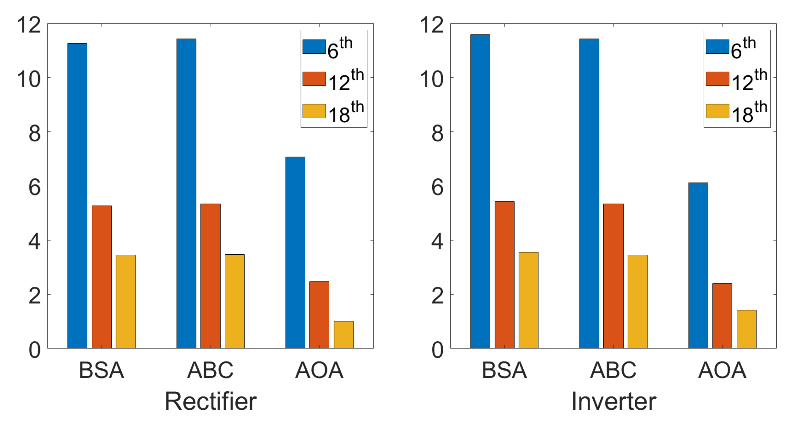
Figure 10.
Voltage profiles for Case 3 and Case 4.

Figure 11.
Comparison of , , , and for Case 3 and Case 4.
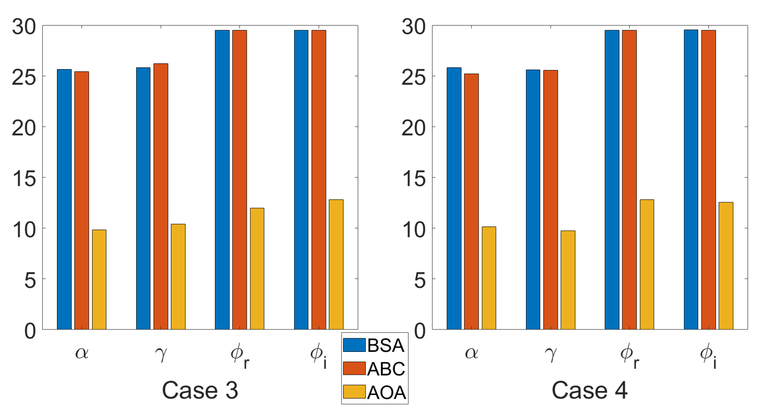
Figure 12.
Harmonics in DC voltages in Case 3.

Figure 13.
Harmonics in DC voltages in Case 4.


Table 1.
Description of case studies.
| Test System | HVDC Link | Without DG | With DG | |
|---|---|---|---|---|
| Rectifier Bus | Inverter Bus | |||
| IEEE 30 bus system | 2 | 14 | Case 1 | Case 3 |
| 2 | 16 | Case 2 | Case 4 | |
Table 2.
Optimized CV with corresponding state variables and comparison of results for Case 1 and Case 2.
Table 2.
Optimized CV with corresponding state variables and comparison of results for Case 1 and Case 2.
| Case 1 | Case 2 | |||||
|---|---|---|---|---|---|---|
| Variable | BSA [28] | ABC [29] | AOA | BSA [28] | ABC [29] | AOA |
| 1.4000 | 1.3211 | 1.4000 | 1.40 | 1.39982 | 1.4000 | |
| 1.0821 | 1.086 | 1.0821 | 1.0788 | 1.1000 | 1.0841 | |
| 1.0626 | 1.072 | 1.0671 | 1.0624 | 1.0614 | 1.0734 | |
| 0.4000 | 0.3600 | 0.3265 | 0.38 | 0.40 | 0.2935 | |
| 0.4000 | 0.4000 | 0.3956 | 0.40 | 0.40 | 0.4000 | |
| 0.2400 | 0.2400 | 0.2400 | 0.24 | 0.18 | 0.2400 | |
| 0.2400 | 0.0900 | 0.2399 | 0.24 | 0.17 | 0.1236 | |
| t(6–9) | 0.96 | 0.99 | 1.01 | 1.00 | 0.96 | 1.00 |
| t(6–10) | 1.05 | 1.08 | 0.90 | 0.91 | 0.94 | 0.92 |
| t(4–12) | 0.97 | 0.94 | 1.00 | 0.98 | 0.96 | 0.98 |
| t(28–27) | 0.97 | 0.98 | 0.96 | 0.94 | 1.00 | 0.97 |
| 0.3074 | 0.1261 | 0.2740 | 0.2782 | 0.4210 | 0.3940 | |
| 0.3025 | 0.1254 | 0.2710 | 0.2746 | 0.4136 | 0.3890 | |
| 0.1537 | 0.0631 | 0.0580 | 0.1391 | 0.2105 | 0.0850 | |
| 0.1513 | 0.0627 | 0.0470 | 0.1373 | 0.2068 | 0.0760 | |
| 0.2540 | 0.100 | 0.1853 | 0.2181 | 0.3129 | 0.2655 | |
| 1.1912 | 1.2539 | 1.4659 | 1.2592 | 1.3219 | 1.4678 | |
| 1.2102 | 1.2614 | 1.4790 | 1.2755 | 1.3453 | 1.4870 | |
| 1.5585 | 1.6375 | 1.5513 | 1.55249 | 1.56880 | 1.5495 | |
| 0.1264 | 0.0318 | 0.0058 | 0.05625 | 0.59452 | −0.0637 | |
| 0.2671 | 0.4248 | 0.2638 | 0.3328 | 0.02932 | 0.5000 | |
| 1.0328 | 1.035 | 1.0303 | 1.0296 | 1.0298 | 1.0313 | |
| 1.0294 | 1.031 | 1.0336 | 1.0269 | 1.0251 | 1.0355 | |
| 1.0949 | 1.076 | 1.0937 | 1.0914 | 1.0845 | 1.0951 | |
| 1.0676 | 1.046 | 1.0783 | 1.0730 | 1.0549 | 1.0531 | |
| 0.94 | 0.97 | 1.05 | 0.99 | 1.05 | 1.05 | |
| 0.96 | 1.02 | 1.05 | 1.02 | 1.08 | 1.07 | |
| 25.5893 | 25.855 | 11.1700 | 25.5899 | 25.9525 | 10.9570 | |
| 25.5952 | 26.387 | 8.6450 | 26.4719 | 25.8957 | 9.5580 | |
| 26.5651 | 26.5832 | 11.9519 | 26.5651 | 26.5651 | 12.1742 | |
| 26.5726 | 26.5651 | 9.8391 | 26.5651 | 26.5651 | 11.0548 | |
| 11.9679 | 12.3874 | 11.4700 | 11.4923 | 11.9300 | 11.0246 | |
Table 3.
Parametric analysis for Case 1 and Case 2.
| Scenarios | Parameter Value | (MW) | ||||
|---|---|---|---|---|---|---|
| Case 1 | Case 2 | |||||
| 1 | 1 | 2 | 1 | 0.5 | 12.0107 | 11.5050 |
| 2 | 1 | 2 | 1 | 1 | 13.1057 | 13.0687 |
| 3 | 1 | 2 | 2 | 0.5 | 11.7952 | 11.5628 |
| 4 | 1 | 2 | 2 | 1 | 12.1605 | 11.4449 |
| 5 | 1 | 4 | 1 | 0.5 | 11.7125 | 11.0981 |
| 6 | 1 | 4 | 1 | 1 | 12.5809 | 11.9604 |
| 7 | 1 | 4 | 2 | 0.5 | 11.5763 | 11.1384 |
| 8 | 1 | 4 | 2 | 1 | 11.5254 | 11.0643 |
| 9 | 1 | 6 | 1 | 0.5 | 11.6948 | 11.1663 |
| 10 | 1 | 6 | 1 | 1 | 12.3014 | 11.7696 |
| 11 | 1 | 6 | 2 | 0.5 | 11.5007 | 11.0332 |
| 12 | 1 | 6 | 2 | 1 | 11.5002 | 11.0379 |
| 13 | 2 | 2 | 1 | 0.5 | 11.7392 | 11.1290 |
| 14 | 2 | 2 | 1 | 1 | 11.8307 | 12.2741 |
| 15 | 2 | 2 | 2 | 0.5 | 11.9015 | 11.2261 |
| 16 | 2 | 2 | 2 | 1 | 12.2811 | 11.3594 |
| 17 | 2 | 4 | 1 | 0.5 | 11.9269 | 11.1986 |
| 18 | 2 | 4 | 1 | 1 | 11.9347 | 11.4218 |
| 19 | 2 | 4 | 2 | 0.5 | 11.6119 | 11.0854 |
| 20 | 2 | 4 | 2 | 1 | 11.5357 | 11.0796 |
| 21 | 2 | 6 | 1 | 0.5 | 11.6670 | 11.5911 |
| 22 | 2 | 6 | 1 | 1 | 12.8450 | 11.4789 |
| 23 | 2 | 6 | 2 | 0.5 | 11.4700 | 11.0246 |
| 24 | 2 | 6 | 2 | 1 | 11.5045 | 11.0405 |
Table 4.
Reduction factor of the harmonic components in AC current in Case 1.
| Order of Harmonics | Rectifier | Inverter | ||||
|---|---|---|---|---|---|---|
| BSA [28] | ABC [29] | AOA | BSA [28] | ABC [29] | AOA | |
| 5th | 0.9995 | 0.9999 | 0.9988 | 0.9994 | 0.9999 | 0.9982 |
| 7th | 0.9991 | 0.9999 | 0.9976 | 0.9988 | 0.9998 | 0.9964 |
| 11th | 0.9977 | 0.9997 | 0.9941 | 0.9970 | 0.9996 | 0.9911 |
| 13th | 0.9967 | 0.9996 | 0.9917 | 0.9959 | 0.9995 | 0.9875 |
Table 5.
Reduction factor of the harmonic components in AC current in Case 2.
| Order of Harmonics | Rectifier | Inverter | ||||
|---|---|---|---|---|---|---|
| BSA [28] | ABC [29] | AOA | BSA [28] | ABC [29] | AOA | |
| 5th | 0.9997 | 0.9994 | 0.9832 | 0.9996 | 0.9992 | 0.9968 |
| 7th | 0.9994 | 0.9989 | 0.9673 | 0.9992 | 0.9985 | 0.9938 |
| 11th | 0.9984 | 0.9972 | 0.9204 | 0.9981 | 0.9964 | 0.9847 |
| 13th | 0.9978 | 0.9961 | 0.8899 | 0.9973 | 0.9949 | 0.9786 |
Table 6.
Performance parameters of converters in Case 1.
| Performance Parameters | Rectifier | Inverter | ||||
|---|---|---|---|---|---|---|
| BSA [28] | ABC [29] | AOA | BSA [28] | ABC [29] | AOA | |
| FF | 1.0116 | 1.0119 | 1.0029 | 1.0116 | 1.0125 | 1.0022 |
| RF | 0.1530 | 0.1549 | 0.0761 | 0.1530 | 0.1583 | 0.0659 |
| TDD | 23.32 | 23.39 | 23.20 | 23.30 | 23.39 | 23.10 |
| TUF | 0.1833 | 0.0752 | 0.1634 | 0.1804 | 0.0748 | 0.1616 |
| VUF | 1.3497 | 1.2949 | 1.1044 | 1.3712 | 1.3027 | 1.1143 |
Table 7.
Performance parameters of converters in Case 2.
| Performance Parameters | Rectifier | Inverter | ||||
|---|---|---|---|---|---|---|
| BSA [28] | ABC [29] | AOA | BSA [28] | ABC [29] | AOA | |
| FF | 1.0116 | 1.0120 | 1.0033 | 1.0125 | 1.0119 | 1.0025 |
| RF | 0.1531 | 0.1552 | 0.0810 | 0.1586 | 0.1548 | 0.0706 |
| TDD | 23.35 | 23.31 | 21.45 | 23.34 | 23.28 | 22.91 |
| TUF | 0.1659 | 0.2510 | 0.2349 | 0.1637 | 0.2466 | 0.2319 |
| VUF | 1.2806 | 1.2142 | 1.0985 | 1.2972 | 1.2357 | 1.1128 |
Table 8.
Optimized CV with corresponding state variables and comparison of results for Case 3 and Case 4.
Table 8.
Optimized CV with corresponding state variables and comparison of results for Case 3 and Case 4.
| Case 3 | Case 4 | |||||
|---|---|---|---|---|---|---|
| Variable | BSA [28] | ABC [28] | AOA | BSA [28] | ABC [28] | AOA |
| 1.4000 | 1.28270 | 1.4000 | 1.4000 | 1.18985 | 1.3996 | |
| 1.078 | 1.073 | 1.0737 | 1.075 | 1.049 | 1.0823 | |
| 1.063 | 1.049 | 1.0724 | 1.058 | 1.027 | 1.0687 | |
| 0.26 | 0.40 | 0.3037 | 0.40 | 0.31 | 0.2601 | |
| 0.36 | 0.29 | 0.3021 | 0.35 | 0.40 | 0.3868 | |
| 0.16 | 0.20 | 0.2357 | 0.24 | 0.24 | 0.1747 | |
| 0.24 | 0.23 | 0.2393 | 0.24 | 0.19 | 0.1510 | |
| t(6–9) | 0.96 | 0.97 | 1.02 | 1.01 | 0.94 | 1.00 |
| t(6–10) | 0.92 | 0.91 | 0.90 | 0.90 | 0.91 | 0.90 |
| t(4–12) | 1.03 | 0.97 | 1.00 | 0.97 | 0.96 | 0.98 |
| t(28–27) | 0.98 | 0.95 | 0.97 | 0.99 | 0.90 | 0.95 |
| DG1 size(loc) | 10.00 (5) | 10.00 (5) | 10.00 (30) | 9.50 (5) | 9.75 (5) | 10.00 (30) |
| DG2 size(loc) | 10.00 (19) | 9.75 (19) | 10.00 (7) | 7.25 (21) | 8.75 (19) | 10.00 (19) |
| DG3 size(loc) | 6.75 (30) | 9.25 (25) | 10.00 (5) | 10.00 (30) | 8.00 (30) | 10.00 (5) |
| 0.2500 | 0.2604 | 0.2650 | 0.3462 | 0.4320 | 0.4360 | |
| 0.2472 | 0.2566 | 0.2620 | 0.3409 | 0.4213 | 0.4300 | |
| 0.1250 | 0.1302 | 0.0570 | 0.1731 | 0.2160 | 0.0900 | |
| 0.1236 | 0.1283 | 0.0480 | 0.1705 | 0.2106 | 0.0850 | |
| 0.1940 | 0.2246 | 0.1767 | 0.2651 | 0.3773 | 0.2916 | |
| 1.2743 | 1.1422 | 1.4875 | 1.2859 | 1.1167 | 1.4758 | |
| 1.2888 | 1.1591 | 1.5000 | 1.3058 | 1.1450 | 1.4970 | |
| 1.26162 | 1.36131 | 1.2209 | 1.25923 | 1.48930 | 1.2208 | |
| 0.11841 | 0.25962 | −0.2188 | 0.12143 | 0.18268 | 0.0646 | |
| 0.38353 | 0.15983 | 0.5000 | 0.25626 | 0.41020 | 0.3538 | |
| 1.019 | 1.022 | 1.0375 | 1.033 | 0.990 | 1.0288 | |
| 1.020 | 1.010 | 1.0335 | 1.026 | 0.991 | 1.0344 | |
| 1.077 | 1.088 | 1.0882 | 1.085 | 1.094 | 1.0818 | |
| 1.042 | 1.070 | 1.0766 | 1.070 | 1.044 | 1.0616 | |
| 1.00 | 0.91 | 1.06 | 1.02 | 0.92 | 1.06 | |
| 1.05 | 0.92 | 1.07 | 1.04 | 0.92 | 1.07 | |
| 25.6475 | 25.4202 | 11.334 | 25.8082 | 25.2163 | 10.3270 | |
| 25.8038 | 26.1961 | 9.2970 | 25.6037 | 25.5373 | 9.4100 | |
| 29.5167 | 29.5167 | 12.1390 | 29.5167 | 29.5167 | 11.6633 | |
| 29.5167 | 29.5167 | 10.3818 | 29.5242 | 29.5107 | 11.1818 | |
| 9.2298 | 9.4227 | 8.4534 | 8.7459 | 8.9475 | 8.0041 | |
Table 9.
Reduction factor of the harmonic components in AC current in Case 3.
| Order of Harmonics | Rectifier | Inverter | ||||
|---|---|---|---|---|---|---|
| BSA [28] | ABC [28] | AOA | BSA [28] | ABC [28] | AOA | |
| 5th | 0.9997 | 0.9996 | 0.9989 | 0.9997 | 0.9994 | 0.9985 |
| 7th | 0.9994 | 0.9993 | 0.9979 | 0.9993 | 0.9987 | 0.9971 |
| 11th | 0.9986 | 0.9983 | 0.9949 | 0.9983 | 0.9969 | 0.9929 |
| 13th | 0.9980 | 0.9976 | 0.9928 | 0.9977 | 0.9957 | 0.9901 |
Table 10.
Reduction factor of the harmonic components in AC current in Case 4.
| Order of Harmonics | Rectifier | Inverter | ||||
|---|---|---|---|---|---|---|
| BSA [28] | ABC [28] | AOA | BSA [28] | ABC [28] | AOA | |
| 5th | 0.9996 | 0.9988 | 0.9972 | 0.9995 | 0.9985 | 0.9965 |
| 7th | 0.9992 | 0.9977 | 0.9946 | 0.9990 | 0.9971 | 0.9932 |
| 11th | 0.9981 | 0.9944 | 0.9867 | 0.9974 | 0.9927 | 0.9833 |
| 13th | 0.9974 | 0.9922 | 0.9815 | 0.9964 | 0.9899 | 0.9768 |
Table 11.
Performance parameters of converters in Case 3.
| Performance Parameters | Rectifier | Inverter | ||||
|---|---|---|---|---|---|---|
| BSA [28] | ABC [28] | AOA | BSA [28] | ABC [28] | AOA | |
| FF | 1.0117 | 1.0115 | 1.0037 | 1.0119 | 1.0122 | 1.0023 |
| RF | 0.1535 | 0.1520 | 0.0860 | 0.1544 | 0.1568 | 0.0682 |
| TDD | 23.35 | 23.34 | 20.13 | 23.35 | 23.30 | 23.16 |
| TUF | 0.1491 | 0.1553 | 0.1580 | 0.1474 | 0.1530 | 0.1562 |
| VUF | 1.2674 | 1.4092 | 1.0889 | 1.2818 | 1.4301 | 1.0981 |
Table 12.
Performance parameters of converters in Case 4.
| Performance Parameters | Rectifier | Inverter | ||||
|---|---|---|---|---|---|---|
| BSA [28] | ABC [28] | AOA | BSA [28] | ABC [28] | AOA | |
| FF | 1.0119 | 1.0113 | 1.0027 | 1.0117 | 1.0115 | 1.0025 |
| RF | 0.1544 | 0.1505 | 0.0735 | 0.1531 | 0.1524 | 0.0701 |
| TDD | 23.34 | 23.22 | 22.98 | 23.32 | 23.16 | 22.88 |
| TUF | 0.2064 | 0.2576 | 0.2600 | 0.2033 | 0.2512 | 0.2564 |
| VUF | 1.2509 | 1.4266 | 1.0911 | 1.2703 | 1.4627 | 1.1068 |
Disclaimer/Publisher’s Note: The statements, opinions and data contained in all publications are solely those of the individual author(s) and contributor(s) and not of MDPI and/or the editor(s). MDPI and/or the editor(s) disclaim responsibility for any injury to people or property resulting from any ideas, methods, instructions or products referred to in the content. |
© 2023 by the authors. Licensee MDPI, Basel, Switzerland. This article is an open access article distributed under the terms and conditions of the Creative Commons Attribution (CC BY) license (https://creativecommons.org/licenses/by/4.0/).
Share and Cite
MDPI and ACS Style
Patel, C.; Malakar, T.; Sreejith, S. Assessment of Converter Performance in Hybrid AC-DC Power System under Optimal Power Flow with Minimum Number of DC Link Control Variables. Energies 2023, 16, 5800. https://doi.org/10.3390/en16155800
AMA Style
Patel C, Malakar T, Sreejith S. Assessment of Converter Performance in Hybrid AC-DC Power System under Optimal Power Flow with Minimum Number of DC Link Control Variables. Energies. 2023; 16(15):5800. https://doi.org/10.3390/en16155800
Chicago/Turabian StylePatel, Chintan, Tanmoy Malakar, and S. Sreejith. 2023. "Assessment of Converter Performance in Hybrid AC-DC Power System under Optimal Power Flow with Minimum Number of DC Link Control Variables" Energies 16, no. 15: 5800. https://doi.org/10.3390/en16155800
Note that from the first issue of 2016, this journal uses article numbers instead of page numbers. See further details here.