Estimating Energy Consumption of Battery Electric Vehicles Using Vehicle Sensor Data and Machine Learning Approaches

Abstract

Transport electrification, which entails replacing fossil fuel-powered engines with electric drivetrains through the use of electric vehicles (EVs), has been identified as a potential strategy for reducing emissions in the transportation sector. As the adoption of EVs increases, there is a growing need to understand their performance and characteristics, particularly the factors that influence energy consumption under actual driving conditions. This study sought to investigate the actual energy consumption of commercial battery electric vehicles (BEVs) in Thailand by conducting real-world driving tests under various route conditions, including urban and rural route modes. Data collection was performed through the use of onboard diagnostics and global positioning system devices. The result shows that the average energy consumption of the BEVs in this study was 148.03 Wh/km. Moreover, several machine learning (ML) techniques were utilized to analyze the collected dataset to predict energy consumption and identify the key factors influencing energy consumption. A comprehensive investigation of factor significance was carried out by employing a specific algorithm in conjunction with the SHapley Additive exPlanations (SHAP) approach. This investigation provided insights into the influence of battery current and vehicle speed on the energy consumption of BEVs, particularly in the context of urban route conditions. The results of this study provide valuable insights into the energy consumption of BEVs and the factors affecting it, which can aid in improving energy efficiency and informing policy decisions related to transport electrification.

1. Introduction

The issue of global warming, characterized by a rising trend in global temperatures, is widely regarded as a critical concern. The primary cause of this phenomenon is the accumulation of greenhouse gases (GHG), particularly carbon dioxide (CO₂), in the atmosphere. The burning of fossil fuels, specifically in the power generation, industrial, agricultural, and transportation sectors, is the major source of CO₂ emissions. Among these, the transportation sector has emerged as a significant contributor to global GHG emissions, accounting for approximately 25% of total emissions, and showing no signs of abating [1]. In particular, road transport has become a leading contributor to emissions, with the use of vehicles such as cars, trucks, and buses having significant detrimental effects on both the environment and public health due to their emissions of GHG and air pollution caused by fossil fuel combustion. As the global population and economy continue to expand, it becomes increasingly imperative to take into consideration the environmental impact of these vehicles and explore ways to decrease their energy consumption and emissions. The European Union (EU) has taken a leading role in addressing the issue of global warming by devising strategies to decrease emissions from the transportation sector and achieve the objectives of the Paris Climate Agreement. As per the European Commission, CO₂ emissions from new vehicles in the EU are projected to decrease by 55% by the year 2030 as compared with 2021 levels [2]. Furthermore, all new vehicles registered in the EU starting from 2035 must be zero-emission vehicles, resulting in the phasing out of conventional internal combustion engine vehicles (ICEVs), which are the primary source of emissions in the transportation sector. In line with the long-term objectives set forth by the European Green Deal [2], there is a critical imperative to achieve a substantial reduction of approximately 90% in emissions from the transportation sector by 2050. These ambitious targets underscore the urgency and necessity of implementing sustainable measures to combat climate change and foster a greener future in the realm of transportation [3].

Transport electrification, which involves transitioning from fossil fuel-powered engines to electric drivetrains, has been identified as a possible strategy for reducing emissions in the transportation sector. This shift towards a clean and sustainable energy system in transportation holds the potential to significantly decrease emissions. As a result, the promotion of electric vehicles (EVs) has gained traction as a means of reducing CO₂ emissions and addressing the issue of climate change [4]. It is projected that EVs will become the prevalent form of vehicle in the global automotive market by the year 2030–2050, thus effectively phasing out the use of gasoline and diesel-burning engines [5]. By incorporating low-emission drivetrains and utilizing renewable energy sources [6,7], EVs have the potential to significantly decrease emissions from both the transportation sector and power generation. EVs, a type of transport electrification, rely on electric motors powered by rechargeable batteries or a combination of an electric motor and an internal combustion engine, instead of solely traditional gasoline or diesel engines. There are three main types of commercial EVs currently available in the market, including battery electric vehicles (BEVs), hybrid electric vehicles (HEVs), and plug-in hybrid electric vehicles (PHEVs). BEVs, propelled solely by an electric motor, are powered by stored electricity and do not emit tailpipe emissions. HEVs have both electric and gasoline engines, which can be powered individually or simultaneously. PHEVs have a larger battery that can be charged by plugging the vehicle into an electric power outlet and can operate in all-electric mode for a certain distance before switching to the gasoline engine. The various types of EVs available exhibit different characteristics. In recent years, the EV market has experienced rapid growth, with a significant increase in the number of EVs on the road. This growth can be attributed to a range of factors, including the falling costs of EV technology, increased availability of EVs, and supportive government policies. As a result, automotive industries in many countries expect EVs to become the primary powertrain in the car market within the next decade. McKinsey and Company, a global management consulting firm, has analyzed the long-term market dynamics of EV market share towards 2030 and found that the EV market share in China, Europe, and the US could increase by approximately 35 to 50%, 35 to 45%, and 15 to 35%, respectively, compared with 2020 [8].

Even though the EV market has seen significant growth in recent years as a way to promote zero-emission transportation, EVs still make up a small percentage of the global vehicle market. Additionally, the majority of EVs are concentrated in a few countries with high EV market shares, such as China, which accounted for around half of the world’s EVs as of 2021, followed by the EU and the US, which together hold about 40% [9]. Among the commercial EVs, BEVs have been observed to have the lowest environmental impact in the long run as they do not produce emissions from tailpipes and can be powered using renewable energy sources. However, certain factors such as range anxiety, the availability of charging infrastructure, the total cost of ownership, and actual vehicle performance can present barriers for some individuals and businesses [10,11,12]. These challenges stand as an obstruction to transition in the early stage. Nevertheless, as the growth in the EV market, especially BEVs, is expected to expand to all regions globally, countries that aim to encourage the adoption of EVs in their transportation systems should be prepared for this shift and conduct further research to be ready for the new normal. The growing interest in BEVs in recent years can be attributed to their potential to mitigate environmental issues arising from fossil fuel consumption and road transportation emissions. To evaluate the potential and practicality of BEVs, numerous studies have been carried out on various facets of EVs, including battery technology, cost-benefit analysis, vehicle efficiency, and environmental impacts [9,13,14,15,16,17].

Energy consumption estimation models play a crucial role in forecasting and assessing the performance and environmental consequences of diverse vehicle types operating under varying traffic conditions. These models serve as indispensable instruments for comprehending the energy efficiency of different traffic configurations, enabling informed decisions in transportation planning and policymaking [18,19,20,21,22]. Analytical, statistical, and machine learning (ML) models are among the various approaches employed to model the energy consumption of vehicles. The ML approach is a rapidly growing field that utilizes algorithms and large datasets to enable computers to learn and make predictions or decisions [23]. Its applications are wide-ranging and have been found to be particularly useful in the transportation industry for understanding and predicting patterns of consumption and emissions. Using ML algorithms, researchers have been able to identify factors that contribute to energy efficiencies, such as vehicle type, driving behavior, and road conditions. The analysis of large datasets through ML has also allowed for the prediction of future energy consumption and emissions based on associated factors [24,25,26]. This information is vital for transportation planners and policymakers as it can be used to make informed decisions on how to reduce energy consumption and emissions most effectively.

The widespread adoption of EVs has led to a growing need to understand their performance and characteristics, particularly the factors that affect energy consumption under actual driving conditions. To our knowledge, no published reports exist regarding the estimation of energy consumption for various brands of current commercial BEVs available in the early stage of the Thai market. Furthermore, based on our extensive literature review, only a limited number of previous studies have explored the applicability of ML techniques to estimate BEV energy consumption and comprehensively analyze the influential variables that contribute to it. For this reason, this study aims to evaluate the energy consumption of current commercial BEVs, which are considered to have the lowest environmental impact among EV types, using in-vehicle sensors and locational tracking data. Additionally, this study employs ML techniques to analyze the collected data and establish predictive models of energy consumption, as well as identify the significance of the variables impacting energy consumption. The findings and conclusions of this research have the potential to be beneficial for EV users, manufacturers, and policymakers in determining the actual efficiency of BEVs.

The present article is structured into five distinct sections. Section 2 elucidates the experimental protocol employed for real-world driving, outlining the proposed methodology for capturing the actual energy consumption of BEVs. This section encompasses aspects such as vehicle specifications, route selection, data collection devices, and the determination of energy consumption. Section 3 details the ML approach utilized. Subsequently, Section 4 presents the results obtained and provides a comprehensive discussion. Lastly, Section 5 presents the overarching conclusions drawn from the study, providing a concise summary of the research findings.

2. Experimental Procedure

The methodology used for determining the energy consumption of BEVs in this study was carefully designed and implemented according to a standard experimental methodology to ensure accurate and reliable results. In this section, we describe the method in detail, including the vehicle specifications, route modes, data collection devices, and energy consumption calculations. In all the real-world driving tests, the onboard diagnostics (OBD) and global positioning system (GPS) devices were used to continuously log in-vehicle sensor and locational data, respectively, via smartphone applications.

2.1. Vehicle Specifications

The driving data used in this study were collected from a real-world driving test conducted with three BEVs that are popular in Thailand and commonly utilized as medium-sized family vehicles in urban and rural areas. The specifications of the test vehicles are presented in

Table 1. Specifications of test vehicles.

Details	BEV1	BEV2	BEV3
Body type	SUV	SUV	C segment
Model year	2019	2020	2018
Electric motor	Permanent-magnet synchronous	Permanent-magnet synchronous	Alternating current synchronous
Motor power (kW)	110	102	110
Battery type	Lithium iron	Lithium iron	Lithium iron
Battery capacity (Wh)	44.50	47.79	40.00
Curb weight (kg)	1535	1510	1580

.

2.2. Route Modes

The test routes for this study were located primarily in Chiang Mai, a city in Thailand with a diverse range of terrain and road types. For a realistic evaluation of energy consumption under actual driving conditions, the routes were selected and classified based on environmental and traffic conditions, in accordance with the European Real Driving Emissions (RDE) test for quasi-flat roads. The routes were differentiated by vehicle speed range, with the urban mode covering speeds below 60 km/h and the rural mode covering speeds between 60 and 90 km/h, both requiring a trip distance of over 16 km and cumulative positive altitude not exceeding 1200 m/100 km [27]. The urban mode focused on traffic-related factors such as light, medium, and heavy congestion. Tests in this mode were conducted in six city areas across various provinces in Thailand, including Chiang Mai, Lampang, Tak, Kamphaeng Phet, Nakhon Sawan, Bangkok, and Phuket. The rural mode aimed to replicate driving conditions on roads in addition to those of the urban mode. These routes were selected to provide a representative sample of different road conditions and speed ranges, such as the changes in curves and elevation of long routes. All round trips in this mode covered a minimum distance of 20 km. The use of RDE test methods and this specific route classification ensures a rigorous and accurate assessment of the energy consumption of BEVs in real-world scenarios. In order to obtain results that truly reflect actual driving conditions, all available vehicle auxiliaries such as music players, air conditioners, and power supplies for mobile devices were used as per normal usage in reality. The total distance traveled by the test vehicles across all trips in all route modes exceeded 7000 km. The experimental design of this study included conducting tests over a three-month period, encompassing both weekdays and weekends. The ambient temperature during testing varied between 26 °C and 31 °C, and the altitudes, relative to sea level, ranged from −10 to 400 m.

2.3. Data Collection Devices

The utilization of sensors and diagnostic tools in commercial vehicles has been on the rise in recent times as these devices are essential for monitoring the performance of the vehicle and ensuring safe and efficient operation by facilitating the diagnosis and monitoring of essential vehicle components, i.e., the engine control module, transmission control module, electronic control units, and various sensors. The most recent version of the OBD system, the second generation of OBD (OBD-II), is an advanced version that employs standardized commands to communicate with other devices within the vehicle. The widespread adoption of Bluetooth technology has made access and control of the OBD system more accessible. Many research studies have employed OBD-II devices to capture and log data from in-vehicle sensors, making the OBD system a vital enabler for various vehicle applications [28,29]. In this study, it was assumed that the use of the OBD system does not affect the energy consumption of the vehicle as it has low energy demands [30].

2.4. Determination of Energy Consumption and Emissions

The electric consumption of BEVs is commonly calculated by measuring the corresponding battery current and voltage, typically in terms of watt-hour per kilometer (Wh/km). The determination of the electric energy consumed by BEVs during a trip in the unit of watt-hour (Wh) can be analyzed from in-vehicle sensor data related to the battery information as follows [30]:

$$E_{\mathrm{trip}}=\frac{1}{3600}{\displaystyle \sum }_{i=1}^n{V}_i\times I_i i=1, 2, 3,\dots ., n$$

(1)

where $V_i$ and $I_i$ denote the battery voltage and current measured at second $i$, while $n$ denotes the last second of a trip. Afterward, the energy consumption $EC$ of BEVs in the unit of Wh/km can be computed by

$$EC=\frac{E_{\mathrm{trip}}}{d_{\mathrm{trip}}}$$

(2)

where $d_{\mathrm{trip}}$ is the total distance of the travel trip in the unit of km.

Furthermore, to assess the environmental impact of BEVs, it is possible to employ a carbon lifecycle analysis as a means to estimate the overall carbon emissions. In the case of BEVs, the carbon pathway primarily encompasses the production, processing, and distribution of electric energy sources. By utilizing a conversion factor, the carbon emissions of BEVs can be calculated based on their energy consumption. According to the guidelines provided by the Thailand Greenhouse Gas Management Organization [31], a BEV’s energy consumption in terms of kWh/km can be approximately converted into the amount of carbon emissions in grams of CO₂ equivalent per kilometer (gCO₂eq/km) using a factor of 598.6 gCO₂eq/kWh.

3. Machine Learning Method

In this study, the development of predictive models was achieved by studying the collected dataset of in-vehicle sensor data and applying ML techniques to investigate patterns and insights that affect the EV’s energy consumption. In the ML process, preprocessing the raw data was performed before creating the model to ensure that only useful data were incorporated into the models. Moreover, the process of selecting suitable algorithms was undertaken to ensure the congruence between the model and the unique demands and characteristics of the dataset.

3.1. Data Collection and Preprocessing

A comprehensive driving dataset comprising approximately 35,000 short-trip data points was acquired, leveraging a diverse range of in-vehicle sensors connected to the OBD-II system. GPS technology was employed to accurately track the vehicle’s location throughout the data collection process. This dataset encompassed multiple BEVs, with careful consideration given to the variables that impact their energy consumption. Data acquisition occurred at a consistent frequency of 1 Hz, ensuring the reliable capture of observed variables, including vehicle speed, acceleration, road slope, battery current, and state of charge.

In order to mitigate the impact of varying ranges among the input features, a standardization process was conducted prior to analysis. Furthermore, to enhance the normal distribution characteristics of the dataset, the Yeo–Johnson non-linear transformation technique was applied [23]. These preprocessing steps significantly contribute to both the stability and expediency of the training process. By standardizing the input features and achieving a normal distribution, potential biases and distortions within the data are minimized, ensuring robustness and facilitating efficient model training.

3.2. Machine Learning Algorithms and Model Evaluation

This study employed four popular and efficient ML algorithms, including Extreme Gradient Boosting (XGB), Random Forest (RF), Multilayer Perceptron (MLP), and Support Vector Regression (SVR) for modeling purposes. The performance of these algorithms on the feature input and target output dataset was assessed using the ten-fold cross-validation method, in which the data are divided into ten subsets, with nine subsets utilized for model training and the remaining one for validation, as shown in Figure 1. Consequently, the training process is carried out with ten loops, and the accuracy of the training process was computed as the mean of those from all the training loops [32,33]. The utilization of the ten-fold cross-validation method allows for a reliable evaluation of the generalization ability of an ML model and can aid in identifying the optimal set of hyperparameters for a given dataset.

The assessment of ML model accuracy constitutes a crucial step in the model development process. Performance evaluation metrics, namely the Coefficient of Determination (R-Squared, ${\mathrm{R}}^2$), Root Mean Squared Error (RMSE), and Mean Absolute Percentage Error (MAPE), were employed to gauge the effectiveness of these models. In order to provide an objective comparison of the estimation model’s performance within this study, these evaluation metrics were utilized. The equations for calculating these metrics can be expressed as follows:

$${\mathrm{R}}^2=1-\frac{{{\displaystyle \sum }}_{i=1}^n{\left(E{C}_i^P-E{C}_i^R\right)}^2}{{{\displaystyle \sum }}_{i=1}^n{\left(E{C}_i^R-\mathrm{mean}\left(E{C}_i^R\right)\right)}^2}.$$

(3)

$$\mathrm{RMSE}=\sqrt{\frac{{{\displaystyle \sum }}_{i=1}^n{\left(E{C}_i^P-E{C}_i^R\right)}^2}{n}}$$

(4)

$$\mathrm{MAPE}=\frac{1}{n} {\displaystyle \sum }_{i=1}^n\left|\frac{E{C}_i^P-E{C}_i^R}{E{C}_i^R}\right|.$$

(5)

Here, $E{C}_i^P$ is the predicted energy consumption, $E{C}_i^R$ denotes the associated real-world energy consumption measured with identical parameters, and $n$ stands for the number of samples. Generally, a higher value of ${\mathrm{R}}^2$ and lower values of RMSE and MAPE indicate superior model performance as they signify a reduced discrepancy between the predicted and actual outcomes. These evaluation metrics serve as reliable indicators of the model’s accuracy, with larger ${\mathrm{R}}^2$ values denoting a stronger correlation and smaller RMSE and MAPE values reflecting decreased errors in the predictions compared with the ground truth.

4. Results and Discussion

4.1. Real-World Energy Consumption

The test routes in this study include a variety of driving conditions, which can be classified as urban and rural routes based on the RDE test. With more than 80 trips, a large number of data points were collected for the variables related to energy consumption. To accurately determine the energy consumption of the vehicles under real-world driving conditions, the energy consumption was estimated using numerous short-distance trips. This approach allows for more accurate capture of variations in energy consumption than considering the average of an entire trip. Figure 2 illustrates the energy consumption of the BEVs against average travel speed.

When evaluating the energy consumption of the BEVs based on route modes, the average consumption was found to be 159.90 Wh/km and 132.24 Wh/km for the urban and rural modes, respectively. It was observed that the consumption of BEVs was higher in the urban mode than in the rural mode, with a difference of 20.92%. A comparison of the individual BEVs on urban routes revealed that BEV2 consumed the highest energy among the BEVs, while BEV1 and BEV3 had similar consumption values. The data also indicated that energy consumption fluctuated greatly in the urban mode, while it was more consistent in the rural mode. Overall, the average energy consumption of the BEVs in this study was determined to be 148.03 Wh/km, as measured across all speed ranges and tests, as shown in Figure 2. It is important to note that Figure 2 visually represents the real-world driving data pertaining to numerous short-distance trips across various average speed ranges. The classification of route modes can be determined by considering the specific speed ranges associated with the data.

Moreover, considering the energy consumption of BEVs, the average carbon emissions were determined to be 95.72 and 79.19 gCO₂eq/km for the urban and rural modes, respectively. The results of this investigation demonstrate that compared with the emissions of ICEVs reported in the literature [14], the BEVs exhibited a reduction in emissions of approximately 60% and 56% in urban and rural settings, respectively.

4.2. Input Features

In this study, Pearson correlation analysis was employed to evaluate the variables associated with the real-world energy consumption of the test vehicles. The objective of utilizing this technique was to identify and eliminate variables that exhibit high correlations with one another. Such variables can pose a challenge in regression models, as they tend to result in unstable and unreliable coefficients. By eliminating these highly correlated variables, the interpretability and stability of the ML models can be improved. In this study, variables with absolute values of the Pearson coefficient greater than 0.8 were removed as they were considered to have a high degree of correlation. The set of input variables (features) selected for the ML models includes vehicle speed, acceleration, road slope, battery current, and state of charge, while the target variable is energy consumption. The values, mean values, and standard deviation (SD) of the input and output variables are presented in

Table 2. Statistical data of the features.

Feature	Unit	Range	Mean	SD
Speed ($v$)	km/h	1.00, 138.61	53.2915	32.2183
Acceleration ($a$)	m/s2	−5.79, 15.99	0.0508	0.6404
Road slope ($m$)	%	−69.85, 69.98	0.0611	10.8670
Battery current ($I$)	A	−246.20, 335.10	11.0517	43.0538
State of charge ($SOC$)	%	13.20, 97.97	50.4685	22.2618

. Note that all data collected from the experiment were used for ML processing.

4.3. Model Selection

Assessing the accuracy of ML models plays a vital role in the process of selecting an optimal model. In the context of this study, various evaluation metrics, including ${\mathrm{R}}^2$, RMSE, and MAPE, were utilized to evaluate the performance of the proposed ML models in predicting the energy consumption of the BEVs. These evaluation metrics provide unique insights into the model’s fit within the framework of a regression model. By employing these metrics, the most effective model can be identified, facilitating the analysis of the influential variables that contribute to the energy consumption. This rigorous evaluation process enables researchers to make informed decisions regarding model selection and gain a deeper understanding of the factors that impact BEV energy consumption.

Table 3. Performance metrics and run times of the considered ML algorithms.

ML Algorithm	Route Mode	${\mathrm{R}}^2$	RMSE	MAPE	Run Time (Second)
XGB	Urban	0.9136 (0.0171)	54.6055 (6.0350)	0.4373 (0.2266)	57.0548
	Rural	0.8380 (0.0211)	34.6301 (2.4754)	0.4180 (0.2330)	45.1028
RF	Urban	0.9261 (0.0113)	51.9839 (4.5549)	0.1181 (0.0049)	56.7060
	Rural	0.8563 (0.0222)	33.2777 (2.8756)	0.2460 (0.1334)	48.6161
MLP	Urban	0.9221 (0.0209)	53.3689 (7.7778)	0.2448 (0.0642)	203.1225
	Rural	0.8400 (0.0168)	35.0335 (2.0151)	0.3015 (0.1016)	120.4364
SVR	Urban	0.3289 (0.0806)	109.3919 (7.2751)	1.2344 (0.4907)	318.6580
	Rural	0.6994 (0.0356)	42.4560 (2.8301)	0.2441 (0.0794)	218.8431

Note: The standard deviation is shown in brackets, (SD).

presents the predictive models’ accuracy in terms of the evaluation metrics and run times. Again, to assess the selected ML algorithms, a comprehensive grid search with a nested ten-fold cross-validation is conducted to determine the optimal hyperparameters. Each training loop’s accuracy is evaluated based on the metrics presented in Table 3, with the average scores and their SDs (indicated in parentheses) provided to gauge the model’s overall performance. Notably, all the models exhibit comparable ${\mathrm{R}}^2$ and RMSE values, except for the SVR model, which stands out with very poor performance outcomes. The achieved high accuracy scores are in line with expectations, considering the utilization of appropriate algorithms and the substantial volume of input data points used for training. Among the ML models, the XGB and RF models exhibit commendable scores in terms of evaluation metrics and run-time efficiency, while the MLP model demonstrates a favorable metric score but requires a longer run time. Conversely, it is worth noting that the SVR model appears unsuitable for this particular dataset.

The RF model exhibits exceptional ${\mathrm{R}}^2$ scores, indicating a robust fit of the model to the data in terms of linear regression. The high percentage values obtained from the RF model emphasize the strong correlation and coherence between the predicted and measured data. These results underscore the efficacy of the RF model in capturing the underlying relationships and patterns within the dataset. On the other hand, the RF model demonstrates the lowest RMSE scores, indicating a superior fit between the predicted and measured data. The excellent absolute measure of fit suggests that the standard deviation of the data variance is minimal. Furthermore, the RF model also exhibits the lowest MAPE scores, which provide an indication of the average percentage difference between the predicted and measured data. As shown in Table 3, the MAPE scores for the RF model in predicting energy consumption under urban and rural modes reveal average deviations of 11.81% and 24.60%, respectively, from the measured values. These evaluation scores indicate that the RF model delivers the most accurate predictions for the dataset examined in this study. It is worth noting that the RF model’s superior performance in terms of accuracy makes it a reliable tool for estimating energy consumption in both urban and rural driving modes. The excellent evaluation scores suggest that the predicted values align closely with the actual energy consumption values, signifying the model’s ability to capture the underlying patterns and factors influencing energy consumption accurately.

Given the satisfactory accuracy achieved by most models, the ML implementation in this study adopts the model with the best performance in accuracy and run time. Consequently, the RF algorithm is chosen to establish the predictive model. The predicted values of energy consumption generated by the chosen ML model were compared with the measured values, the red square dots, as shown in Figure 3. The diagonal lines in the figures represent the ideal estimation, while the green and blue lines indicate error boundaries of $\pm$10% and $\pm$20%, respectively. Most of the results were found to fall along the diagonal line within the green line boundary, indicating the accuracy of the predictive models. The difference between the measured and predicted results for the urban mode showed more fluctuation than that of the rural mode, with some results outside the 10% error region. Additionally, a few results were observed beyond the 20% error lines. Figure 3a provides visual evidence of the significant presence of highly scattered consumption data within the range of 300 to 1000 Wh/km for the urban mode. Conversely, Figure 3b reveals that for the rural mode, the consumption data are primarily concentrated within the −400 to 600 Wh/km range, suggesting a comparatively lower rate of energy consumption in this route mode.

4.4. Feature Importance

Determining feature importance is a critical step in the ML approach as it enables a deeper understanding of the extent to which features influence the target variable. This knowledge not only enhances interpretability but also provides valuable insights into the intricate relationships between features and the target variable. Given the complexity of estimating energy consumption, which is influenced by a multitude of variables, a feature importance analysis was conducted using the RF algorithm in conjunction with SHapley Additive exPlanations (SHAP) method. SHAP is a game-theoretic approach used to elucidate a model’s output by scoring the contribution of each feature to the predicted results [34]. In this research, the SHAP approach was employed to analyze feature importance and identify the significant impacts of the input variables.

To effectively present the distribution of SHAP values for each feature in the ML model, beeswarm plots were employed, as depicted in Figure 4 and Figure 5. The horizontal axis of the plot represents the range of SHAP scores for the features, while the red and blue contour dots indicate the high and low impact levels, respectively, of these features on the energy consumption of the BEVs. These visual representations allow for a comprehensive understanding of the relative importance and influence of each feature on the energy consumption predictions.

The classification of route modes in this study results in distinct variations in energy consumption ($EC$) of the BEVs. Figure 4 visually presents the SHAP analysis of the energy consumption prediction for the urban route mode, revealing notable findings regarding the impact of input variables $I$ and $v$ on the $EC$. The analysis demonstrates a highly significant influence of both $I$ and $v$, as indicated by their SHAP scores. Evidently, the SHAP scores for $I$ exhibit a relatively uniform distribution, encompassing both positive and negative scores of approximately $\pm$800. This suggests a linear relationship between $I$ and $EC$, with the positive scores associated with high values of $I$ (represented by the red contour dots). Consequently, an increase in $I$ corresponds to an elevation in the $EC$, while a decrease in $I$ results in a decrease in $EC$. Conversely, the SHAP scores for variable $v$ display an uneven distribution, with a range of scores approximately between $-$250 and $+$1000, as depicted in Figure 4. This observation signifies a non-linear relationship between $v$ and $EC$. Positive SHAP scores associated with low values of $v$ indicate that at a lower vehicle speed, the energy consumption increases, and vice versa. However, the degree of change in the negative range is less significant than in the positive range. The varying degrees of change in the positive and negative score ranges highlight the greater significance of low values of $v$ to the energy consumption, which is characteristic of heavy urban traffic conditions. The resulting significant impact of $v$ on energy consumption is consistent with a report in the literature [35] which highlights the strong correlation between vehicle speed and energy consumption, particularly in the ranges of speed below 30 km/h. The state of charge, acceleration, and road slope also exert influences on energy consumption; however, their respective SHAP scores are notably lower in comparison with those of the battery current and vehicle speed.

The SHAP analysis results for the rural route mode are presented in Figure 5. Among the input variables, $I$ demonstrates the most substantial impact on the energy consumption of the BEVs, as evidenced by the highest SHAP score. The SHAP scores for $I$ display a relatively uniform distribution across both positive and negative ranges, approximately $\pm$600. This indicates a linear relationship between $I$ and $EC$, where an increase in $I$ corresponds to an increase in $EC$, and vice versa. However, these findings differ from those of the urban route mode as the SHAP score of $I$ in the rural route mode is clearly lower. Furthermore, in this route mode, the influence of $v$ on $EC$ is significantly diminished, suggesting $v$ is a low-impact feature. The observed positive shift in the analysis results concerning energy consumption demonstrates the efficacy of BEVs in the rural route mode, aligning with both experimental findings and the existing literature. Moreover, the state of charge, acceleration, and road slope can be categorized as features with low impacts on the energy consumption of BEVs in both urban and rural route modes.

5. Conclusions

This study investigated the actual energy consumption of commercial BEVs in Thailand, by conducting real-world driving tests in both urban and rural modes. Moreover, the ML approach was applied to analyze the large amount of data obtained from the tests. This enabled the prediction of energy consumption and the identification of the key factors influencing energy consumption. The following key findings were observed in this study:

• The average energy consumption of the BEVs was found to be 159.90 Wh/km for the urban mode and 132.24 Wh/km for the rural mode, while the overall average consumption was 148.03 Wh/km.
• There was a difference of approximately 21% in the average energy consumption between driving on urban and rural routes.
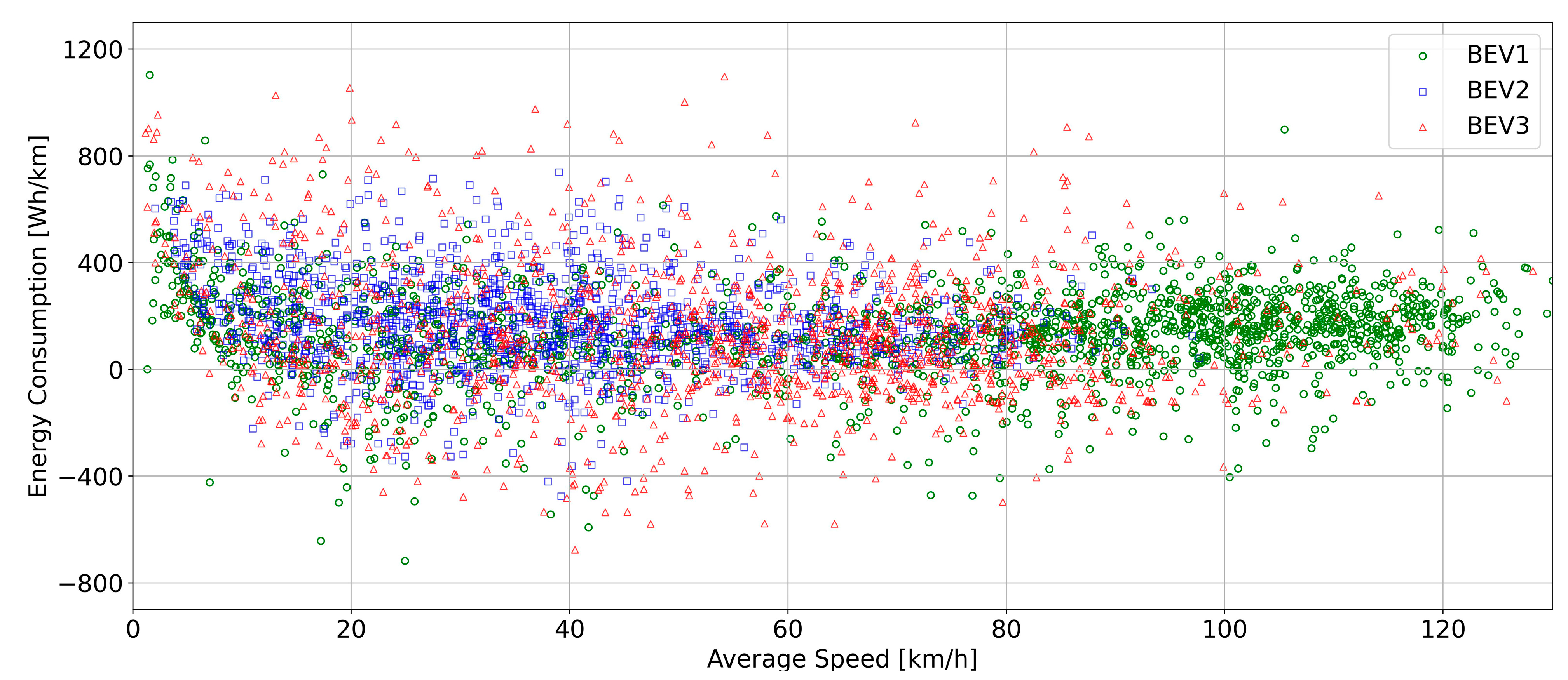
• The BEVs showed higher energy consumption rates in the speed range below 30 km/h.
• The energy consumption of the BEVs has higher fluctuations in the urban route mode.
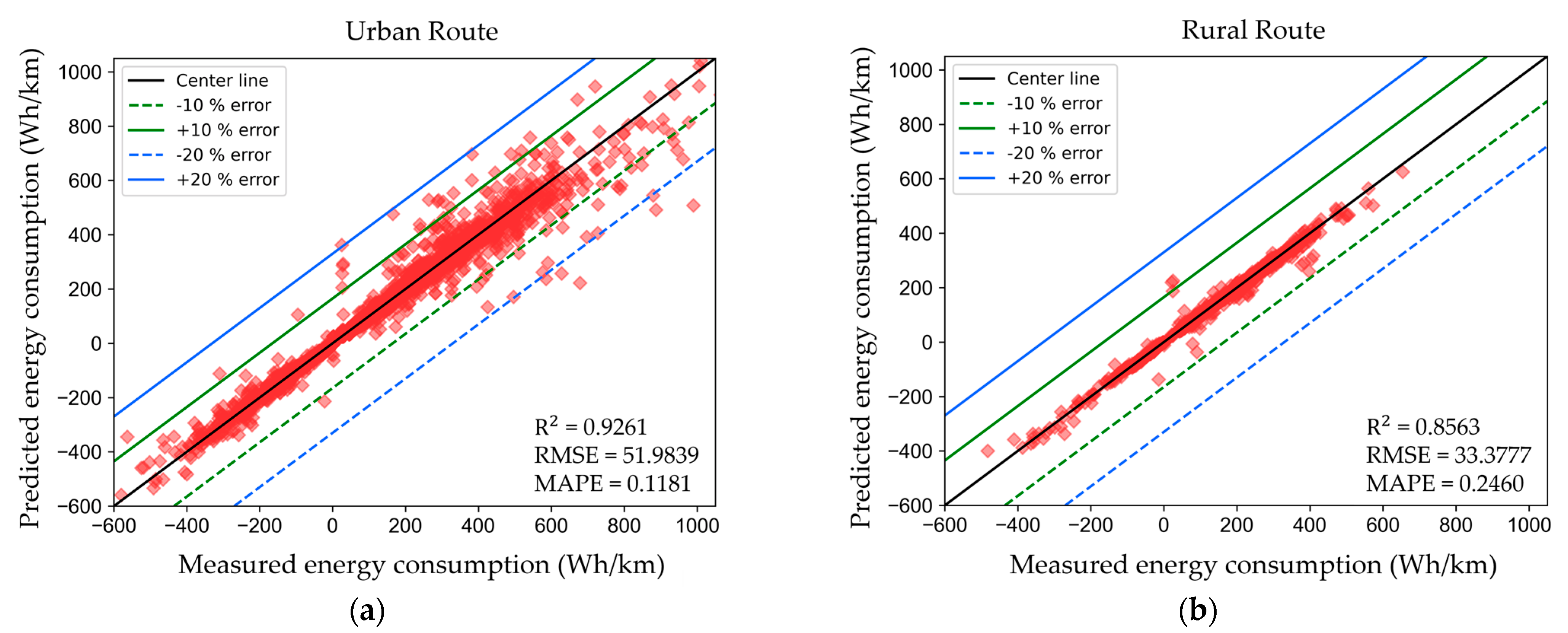
• The RF algorithm demonstrated the best performance in terms of accuracy and run time, with MAPE scores of 11.81 and 24.60% for urban and rural routes, respectively.
• The factors that have an impact on the energy consumption, in descending order, were found to be battery current, speed, state of charge, acceleration, and road slope.

Based on the findings of this study, generalized conclusions can be drawn regarding the substantial influence of traffic conditions on the energy consumption of BEVs. It was observed that BEVs tend to consume more electric power when operating at lower average speeds with frequent fluctuations in acceleration. Furthermore, the utilization of appropriate ML models based on real-world data measurements has demonstrated efficacy in accurately predicting BEV energy consumption. These potential predictive models can be further applied in the development of autonomous control systems for advanced automotive technologies.

References

1. International Energy Agency (IEA). Greenhouse Gas Emissions from Energy Data Explorer. Available online: https://www.iea.org/data-and-statistics/data-tools/greenhouse-gas-emissions-from-energy-data-explorer (accessed on 10 November 2021).
2. European Commission (EC). European Green Deal: Commission Proposes Transformation of EU Economy and Society to Meet Climate Ambitions. Available online: https://ec.europa.eu/commission/presscorner/detail/en/IP_21_3541 (accessed on 14 July 2021).
3. Szaruga, E.; Załoga, E. Qualitative–Quantitative Warning Modeling of Energy Consumption Processes in Inland Waterway Freight Transport on River Sections for Environmental Management. Energies 2022, 15, 4660. [Google Scholar] [CrossRef]
4. Kłos-Adamkiewicz, Z.; Szaruga, E.; Gozdek, A.; Kogut-Jaworska, M. Links between the Energy Intensity of Public Urban Transport, Regional Economic Growth and Urbanisation: The Case of Poland. Energies 2023, 16, 3799. [Google Scholar] [CrossRef]
5. International Energy Agency (IEA). Global Energy Review: CO2 Emissions in 2021. Available online: https://www.iea.org/reports/global-energy-review-co2-emissions-in-2021-2 (accessed on 8 March 2022).
6. Chaichana, C.; Wongsapai, W.; Damrongsak, D.; Ishihara, K.N.; Luangchosiri, N. Promoting community renewable energy as a tool for sustainable development in rural areas of Thailand. Energy Procedia 2017, 141, 114–118. [Google Scholar] [CrossRef]
7. Mona, Y.; Do, T.A.; Sekine, C.; Suttakul, P.; Chaichana, C. Geothermal electricity generator using thermoelectric module for IoT monitoring. Energy Rep. 2022, 8, 347–352. [Google Scholar] [CrossRef]
8. Gersdorf, T.; Hensley, R.; Hertzke, P.; Schaufuss, P. Electric Mobility after the Crisis: Why an Auto Slowdown Won’t Hurt EV Demand. McKinsey & Company. Available online: https://www.mckinsey.com/industries/automotive-and-assembly/our-insights (accessed on 16 September 2020).
9. Ayetor, G.K.; Opoku, R.; Sekyere, C.K.; Agyei-Agyeman, A.; Deyegbe, G.R. The cost of a transition to electric vehicles in Africa: A case study of Ghana. Case Stud. Transp. Policy 2022, 10, 388–395. [Google Scholar] [CrossRef]
10. Donkers, A.; Yang, D.; Viktorović, M. Influence of driving style, infrastructure, weather and traffic on electric vehicle performance. Transp. Res. Part D Transp. Environ. 2020, 88, 102569. [Google Scholar] [CrossRef]
11. Degen, F.; Schütte, M. Life cycle assessment of the energy consumption and GHG emissions of state-of-the-art automotive battery cell production. J. Clean. Prod. 2022, 330, 129798. [Google Scholar] [CrossRef]
12. Suttakul, P.; Wongsapai, W.; Fongsamootr, T.; Mona, Y.; Poolsawat, K. Total cost of ownership of internal combustion engine and electric vehicles: A real-world comparison for the case of Thailand. Energy Rep. 2022, 8, 545–553. [Google Scholar] [CrossRef]
13. Wei, H.; He, C.; Li, J.; Zhao, L. Online estimation of driving range for battery electric vehicles based on SOC-segmented actual driving cycle. J. Energy Storage 2022, 49, 104091. [Google Scholar] [CrossRef]
14. Suttakul, P.; Fongsamootr, T.; Wongsapai, W.; Mona, Y.; Poolsawat, K. Energy consumptions and CO2 emissions of different powertrains under real-world driving with various route characteristics. Energy Rep. 2022, 8, 554–561. [Google Scholar] [CrossRef]
15. Zhang, C.; Yang, F.; Ke, X.; Liu, Z.; Yuan, C. Predictive modeling of energy consumption and greenhouse gas emissions from autonomous electric vehicle operations. Appl. Energy 2019, 254, 113597. [Google Scholar] [CrossRef]
16. Achariyaviriya, W.; Suttakul, P.; Fongsamootr, T.; Mona, Y.; Phuphisith, S.; Tippayawong, K.Y. The social cost of carbon of different automotive powertrains: A comparative case study of Thailand. Energy Rep. 2023, 9, 1144–1151. [Google Scholar] [CrossRef]
17. Pignatta, G.; Balazadeh, N. Hybrid Vehicles as a Transition for Full E-Mobility Achievement in Positive Energy Districts: A Comparative Assessment of Real-Driving Emissions. Energies 2022, 15, 2760. [Google Scholar] [CrossRef]
18. Achariyaviriya, W.; Hayashi, Y.; Takeshita, H.; Kii, M.; Vichiensan, V.; Theeramunkong, T. Can Space–Time Shifting of Activities and Travels Mitigate Hyper-Congestion in an Emerging Megacity, Bangkok? Effects on Quality of Life and CO2 Emission. Sustainability 2021, 13, 6547. [Google Scholar] [CrossRef]
19. Kantavat, P.; Kijsirikul, B.; Iwahori, Y.; Hayashi, Y.; Panboonyuen, T.; Vateekul, P.; Achariyaviriya, W. Transportation Mobility Factor Extraction Using Image Recognition Techniques. In Proceedings of the 2019 First International Conference on Smart Technology & Urban Development (STUD), Chiang Mai, Thailand, 13–14 December 2019; pp. 1–7. [Google Scholar]
20. Kasemset, C.; Boonmee, C.; Arakawa, M. Traffic Information Sign Location Problem: Optimization and Simulation. Ind. Eng. Manag. Syst. 2020, 19, 228–241. [Google Scholar] [CrossRef]
21. Kasemset, C.; Suto, H. A case study of outbound-vehicle analysis in traffic system: Optimization to simulation. In Proceedings of the 2019 IEEE 6th International Conference on Industrial Engineering and Applications (ICIEA), Tokyo, Japan, 12–15 April 2019; pp. 775–779. [Google Scholar]
22. Zhang, Q.; Tian, S. Energy Consumption Prediction and Control Algorithm for Hybrid Electric Vehicles Based on an Equivalent Minimum Fuel Consumption Model. Sustainability 2023, 15, 9394. [Google Scholar] [CrossRef]
23. Katongtung, T.; Onsree, T.; Tippayawong, N. Machine learning prediction of biocrude yields and higher heating values from hydrothermal liquefaction of wet biomass and wastes. Bioresour. Technol. 2022, 344, 126278. [Google Scholar] [CrossRef]
24. Rivera-Campoverde, N.D.; Muñoz-Sanz, J.L.; Arenas-Ramirez, B.d.V. Estimation of pollutant emissions in real driving conditions based on data from OBD and machine learning. Sensors 2021, 21, 6344. [Google Scholar] [CrossRef]
25. Yao, Y.; Zhao, X.; Liu, C.; Rong, J.; Zhang, Y.; Dong, Z.; Su, Y. Vehicle fuel consumption prediction method based on driving behavior data collected from smartphones. J. Adv. Transp. 2020, 2020, 9263605. [Google Scholar] [CrossRef]
26. Basso, R.; Kulcsár, B.; Sanchez-Diaz, I. Electric vehicle routing problem with machine learning for energy prediction. Transp. Res. Part B Methodol. 2021, 145, 24–55. [Google Scholar] [CrossRef]
27. Prati, M.V.; Costagliola, M.A.; Giuzio, R.; Corsetti, C.; Beatrice, C. Emissions and energy consumption of a plug-in hybrid passenger car in Real Driving Emission (RDE) test. Transp. Eng. 2021, 4, 100069. [Google Scholar] [CrossRef]
28. Hien, N.L.H.; Kor, A.-L. Analysis and Prediction Model of Fuel Consumption and Carbon Dioxide Emissions of Light-Duty Vehicles. Appl. Sci. 2022, 12, 803. [Google Scholar] [CrossRef]
29. Frey, H.C.; Zheng, X.; Hu, J. Variability in measured real-world operational energy use and emission rates of a plug-in hybrid electric vehicle. Energies 2020, 13, 1140. [Google Scholar] [CrossRef]
30. Al-Wreikat, Y.; Serrano, C.; Sodré, J.R. Driving behaviour and trip condition effects on the energy consumption of an electric vehicle under real-world driving. Appl. Energy 2021, 297, 117096. [Google Scholar] [CrossRef]
31. Thailand Greenhouse Gas Management Organization (TGO). Emission Factor and Carbon Footprint of Products. Available online: http://thaicarbonlabel.tgo.or.th/index.php?lang=TH&mod=Y0hKdlpIVmpkSE5mWlcxcGMzTnBiMjQ9 (accessed on 12 October 2022).
32. Zhang, H.; Yang, S.; Guo, L.; Zhao, Y.; Shao, F.; Chen, F. Comparisons of isomiR patterns and classification performance using the rank-based MANOVA and 10-fold cross-validation. Gene 2015, 569, 21–26. [Google Scholar] [CrossRef]
33. Ullah, I.; Liu, K.; Yamamoto, T.; Al Mamlook, R.E.; Jamal, A. A comparative performance of machine learning algorithm to predict electric vehicles energy consumption: A path towards sustainability. Energy Environ. 2022, 33, 1583–1612. [Google Scholar] [CrossRef]
34. Ullah, I.; Liu, K.; Yamamoto, T.; Zahid, M.; Jamal, A. Modeling of machine learning with SHAP approach for electric vehicle charging station choice behavior prediction. Travel Behav. Soc. 2023, 31, 78–92. [Google Scholar] [CrossRef]
35. Fetene, G.M.; Kaplan, S.; Mabit, S.L.; Jensen, A.F.; Prato, C.G. Harnessing big data for estimating the energy consumption and driving range of electric vehicles. Transp. Res. Part D Transp. Environ. 2017, 54, 1–11. [Google Scholar] [CrossRef]
Figure 1. Ten-fold cross-validation diagram.
Energies 16 06351 g001
Figure 2. The energy consumption in relation to the average travel speed of the selected BEVs.
Energies 16 06351 g002
Figure 3. Plots of measured versus predicted values of the consumption of the BEVs under different route modes: (a) urban route; (b) rural route.
Energies 16 06351 g003
Figure 4. Beeswarm plot of SHAP values—Features influencing the BEVs’ energy consumption in urban route mode.
Energies 16 06351 g004
Figure 5. Beeswarm plot of SHAP values—Features influencing the BEVs’ energy consumption in rural route mode.
Energies 16 06351 g005