Developed and Intelligent Structure of a Control for PV Water Treatment System


1
Faculty of Sciences of Tunis, University of Tunis El Manar, UR-LAPER, Tunis 1068, Tunisia
2
Unit of Research ERCO-INSATE, National High School of Engineering of Tunis (ENSIT), Tunis 1002, Tunisia
3
Laboratory for Analysis Conception and Control of Systems, LR-11-ES20, Department of Electrical Engineering, National Engineering School of Tunis, Faculty of Sciences of Tunis, University of Tunis El Manar, Box 37, Le Belvedere, Tunis 1002, Tunisia
*
Author to whom correspondence should be addressed.
†
These authors contributed equally to this work.
Energies 2023, 16(18), 6540; https://doi.org/10.3390/en16186540
Submission received: 17 July 2023
/
Revised: 16 August 2023
/
Accepted: 24 August 2023
/
Published: 11 September 2023
(This article belongs to the Section A2: Solar Energy and Photovoltaic Systems)
Abstract
:The subject of this work is a UV-irradiated water disinfection prototype intended for use in rural areas where access to water is difficult. Given the favorable climatic conditions of our country, the use of photovoltaic panels as a source of energy is particularly interesting, and has relevance in regions with a similar climate. PV energy being a fluctuating source that influences water disinfection operations, we have developed a database to distribute the energy available to the loads (UV lamps, electric pumps) in order to ensure a better quality of the water. This database is used in deep learning to model water disinfection phenomena. This method is able to adjust the speed instructions of the motor pump (therefore the flow rate) and the UV irradiation according to the energy available to ensure optimal water quality. Several other techniques have been implemented to control the instructions generated by the deep learning developed, to control the motor, the inverter and the DC/DC converter (IRFOC, SVPWM, sliding mode). All these approaches are tested in real time and they represent good results in terms of water treatment control. The effectiveness of these types of control is proven by the results obtained.
1. Introduction
Recent decades have been marked by energy problems that have become international issues. No one can ignore the fact that the development of a region depends, in large part, on reliable, stable and sustainable energy production and supply. Energy production mainly relies on fossil fuel sources (nearly 80% of total primary energy production in the world [1]) such as oil, coal, gas, etc.
This electrical energy production model will lead in the long term to the depletion of fossil reserves, while nuclear sources pose a permanent risk [2]. Fossil fuels can also create environmental problems such as greenhouse gas emissions including carbon dioxide release. These reasons lead decision-makers and researchers to increasingly consider the use of so-called “green” techniques for the production of electrical energy. These are based on renewable sources such as water, the sun, the wind and biomass fuel. The production of electrical energy by a photovoltaic system is one of the solutions currently adopted. This energy is dependent on many factors such as the inclination of the panels, their technologies, climatic factors, etc.
Photovoltaic generators (PVGs) present a finite and fluctuating energy source, which can span a wide range of output voltages and currents. These PVGs can deliver maximum power only for particular values of current and voltage [2,3]. The efficiency depends on the operating point of the receiver. For optimum operation (maximum power), it is sometimes necessary to insert one or more controlled static converters between the generator and the receiver, allowing operation to be adjusted at the point of maximum power.
Water is an essential resource for the reproduction and maintenance of life. Access to clean water and sanitation is essential for human survival. However, geographic changes and globalization cause rivers to fluctuate. Due to the growth of urban spaces, water is considered a scarce and limited resource. Per capita freshwater availability is likely to deteriorate, especially in rural areas, where scattered settlements and limited energy facilities often make it more difficult to meet water demand. Therefore, all resources must be mobilized, including the storage of rainwater and the extraction of urban groundwater by wells. But if their operations are poorly managed and the water resources are insufficient, these resources can become a factor in the spread of diseases if they are not treated or are treated inadequately [4].
According to the work carried out in the literature, the results of water disinfection mainly depend on the illumination and the water flow, which have a nonlinear relationship. The system examined in this work is powered by a photovoltaic generator. This fluctuating light source makes it impossible to fix constant flux and irradiation. In unfavorable climatic conditions, we cannot have the photovoltaic energy necessary to respect the instructions in order to ensure optimal water quality. Therefore, each change in climatic factors will cause a variation in the PV power, which in turn will influence the flow of water and the UV flux and consequently the quality of the water. Likewise, the control of the system in real time will be very difficult given the absence of sensors indicating the bacteriological quality of the water, and knowing that the bacteriological analysis of the quality of the water requires three days. All these problems already bring us back to using intelligent control based on deep learning. This feature mainly allows us to manage the water treatment system in different climatic conditions. For these reasons, based on experimental tests (bacteriological analysis), we will create a database for the creation of a deep learning system. This deep learning system models the water disinfection phenomena and provides real-time control of the water treatment system according to the energy available. Similarly, the nonlinear relationship between water flow and UV flux has an influence on the management of water treatment in the presence of climatic variation.
Using the database enabled changing the flow rate of the water to be treated from a minimum value to a maximum value. For each flow value, we varied the UV flux. Bacteriological analysis allowed us to determine the UV flux value corresponding to the previously set flow for optimal water quality. We repeated this process until the maximum flow rate and corresponding UV flux values were reached [5].
In this work, we have detailed the different control techniques used, as follows: sliding mode control (MPPT) for the DC/DC converter, sliding mode control for the UV lamp, SVPWM pulse width modulation for the inverter key control and IRFOC command for the motor. These different control and command techniques are all implemented and tested experimentally. In this work, we used deep learning to model the phenomenon of water disinfection (to manage water disinfection based on available energy). This allows the control of the water treatment unit in real time according to the energy available.
This work covers the following points:
- Detailed study and development of a water treatment system with different control approaches;
- Verification and simulation;
- The establishment and implementation of an experimental test bench for the PV water treatment system based on a PVG, a chopper, inverter, motor pump, UV lamp, sensors, etc.;
- Interpretation of the results.
First of all, the results of the simulation clearly show the effectiveness of the control mode chosen for the UV lamp.
Then, the experimental results prove the effectiveness of the different control approaches used.
2. General Structure of PV Water Treatment System
Figure 1 summarizes the general architecture of our system. This structure is mainly composed of a moto-pump and UV lamp supplied by a PV generator via many static converters. These converters are controlled by a duty cycle and PWM signals delivered automatically by an STM32F4 microcontroller.
2.1. PVG Model
The traditional PV cell equivalent circuit is likened to a current source along with a diode, a series resistor and a shunt resistor [6], as shown in Figure 2.
Taking this into account, the current delivered to a load by an illuminated photovoltaic cell is written as:
In the ERCO research unit, we have a photovoltaic generator consisting of ten panels in series of the TITAN-12-50 type. In order to obtain the characteristics of the PVG, the voltage and current quantities are stored in a digital oscilloscope of the Metrix OX7104 type, (ERCO research unit (INSAT) in Tunisia).
Figure 3 shows a recording of the current and voltage quantities for an illumination of 400 W/m2 and a temperature of 28 °C.
These records are transformed into an Excel table and then plotted on MATLAB/Simulink as shown in the following Figure 4.
2.1.1. Effect of Series and Shunt Resistances
The effects of series and shunt resistances on the characteristics are intensively studied in several works such as [7]. In general, the influence of Rs is clear when the generator behaves like a voltage generator, while the influence of Rsh manifests when the generator behaves as a current generator, as shown in Figure 5.
2.1.2. Estimation of Series and Shunt Resistances
To correctly evaluate the energy balance, the estimation of the series resistance and the shunt resistance of the equivalent diagram of the PVG is certainly beneficial.
In order to facilitate the calculation, it is necessary to introduce and define certain sensitivity coefficients in order to arrange the calculation in the simplest and clearest possible way. Let us define the following quantities:
This estimate is based on the use of the equation of the internal conductance of the GPV in any regime, which is variable with the operating point, relationship (5) and the mathematical model given by relationship (6):
The simulation results mentioned above show that the effect of the resistance Rs manifests itself mainly in the vicinity of open voltage operation. In this area, the effect of the shunt resistance is not really significant. So, the estimation of Rs is carried out around a no-load operation while ignoring the effect of Rsh.
For this, we will use the derivatives of these quantities with respect to Vpv and Ipv:
The relationship used to estimate the series resistance is as follows:
with and .
Through the application of Equation (5), we obtained the following relationship:
In STC conditions, we obtain:
The second term of the quantity in square brackets being in practice small compared to unity, the expression of the series resistance could be simplified to:
For the shunt resistance, this can be estimated around the short-circuit operating point while neglecting the effect of Rs. We then pose:
where and .
So, we obtain:
This can also be expressed as:
For the resolution of this quadratic equation, the discriminant was calculated, which involves the square of the saturation current, which is of a very small magnitude. So, we can eliminate the second term of this equation and estimate the shunt resistance by the following relationship:
In STC conditions, we obtain:
2.1.3. Influence of Illumination and Temperature on the Estimated Series Resistance
Considering the relationship (12), at a constant temperature, the series resistance is marked by the inverse of the short-circuit current. As the latter increases proportionally to the illumination, it follows that the resistance Rs varies in the opposite direction to Es. This is well confirmed by the curve in the following Figure 6.
The relationship (11) shows that, at constant illumination, the series resistance is positively proportional to the temperature of the junction. This is quite apparent on the first curve of Figure 7.
2.1.4. Influence of Illumination and Temperature on the Estimated Shunt Resistance
The expression (16) of the shunt resistance gives rise to a term that decreases with the short-circuit current. Moreover, the denominator of this expression is proportional to the saturation current, which is very low. This justifies on the one hand the high values of this resistance at low value of illumination and its decrease on the other hand when Es increases, as shown in Figure 8.
Relationship (17) shows on one side a term proportional to the temperature and on the other side a second term that decreases exponentially with the temperature. This results in the overall decreasing behavior illustrated by the curve in the following Figure 9.
2.2. Optimal Operation of PV System
Solar cells naturally exhibit nonlinear characteristics that vary with solar radiation and temperature, as shown in the Figure 10 and Figure 11 below.
Various publications on MPPT controls have appeared in the literature since 1968, the date of publication of the first control law, adapted to a renewable energy source of the photovoltaic type. These techniques essentially consist in bringing each time the operating point of the photovoltaic generator to the MPP whatever the abrupt variations in the load or the weather conditions [8,9,10,11]. These different techniques are mainly used to control a static DC/DC type converter, which will play the role of an adaptation stage between the source and the load.
2.2.1. Adaptation Stage: DC/DC Converter
Therefore, the insertion of a DC/DC type static converter is necessary. This SCV acts as an adapter between the source and the load in order to reach the maximum power point that corresponds to the optimum power generated by the PV generator.
For the BOOST chopper configuration, the average output voltage is higher than the input voltage, hence its name, booster. This structure requires a switch controlled on triggering and blocking (bipolar, MOS, IGBT, etc.) and a diode (spontaneous triggering and blocking). A booster chopper, as its name suggests, converts a DC voltage into another DC voltage of greater value [12].
Figure 12 shows a block diagram of a parallel chopper. The inductance makes it possible to smooth the current supplied by the source. Capacitor C makes it possible to limit the output voltage ripple. In the case of the present study, the capacitance of the capacitor is taken so that the ripple of the voltage has no effect.
2.2.2. Adopted MPPT Technique: Sliding Mode Control
The MPPT control varies the duty cycle of the static converter (SCV), using an appropriate electrical signal to extract the maximum power that the PVG can provide. The MPPT algorithm can made be more or less complicated in order to find the PPM. In general, this is based on the variation of the duty cycle of the SCV according to the evolution of the input parameters of the latter (Ip and Vp) and consequently of the power of the PVG until it is placed on the MPP.
Sliding mode control is a technique with variable structure, which is mainly characterized by a structure that varies with the evolution of the control according to a very specific switching logic [13,14,15].
The principle of this method essentially consists of constraining the system to reach a given surface called “slip surface” and to remain there until reaching equilibrium. So, the control by sliding mode is carried out in two steps, as shown in Figure 13:
- Convergence towards the sliding surface;
- Sliding along it.
For the sliding surface, we chose the equation that characterizes the incremental conductance method:
At the point of maximum power, this surface satisfies the following relationship:
We considered as an incremental conductance and like an instantaneous inductor. So, we can write the slip surface in another form:
The equivalent ueq command is given by the following relationship:
The nonlinear command a is expressed by Equation (22):
So, we finally obtain the control law:
2.3. Kinetic Modeling of Water Disinfection
All discharge lamps convert electrical energy into light energy by converting electrical energy into kinetic energy of moving electrons, which in turn is converted into electromagnetic radiation by some collision processes with gas atoms (steam) or mixtures thereof. Some of the moving electrons act on the atom so strongly that the internal state of the atom changes (inelastic collision). These changes can be of two types: excitation or ionization. Many models are based on the current–voltage characteristics of high-frequency (>20 kHz) discharges. You are trying to find a function that describes the relationship between the voltage, current and power [16].
Discharge Lamp Model
The discharge conductance can be described using a first-order differential equation:
Therefore, the coefficient can be determined experimentally based on the voltage–current characteristics or physical evaluation (when is 2 or 3). In this case, the coefficients have physical meaning. The conductivity of the discharge can be calculated by the following formula:
where is the current through the discharge lamp, is the discharge voltage, is the specific resistance and is the conductivity of the discharge.
Polynomial models can be used with n = 2 with good results. In this case, the constants a, b1 and b2 will have physical meaning [17].
The lamp voltage and lamp conductance are obtained by solving the differential equations corresponding to the model. The input current i(t) supplied by the electronic ballast is known. There are many options for the shape of the UV lamp; we selected the G type. It can be seen that, even at high frequencies, the polynomial model fits slightly better than the exponential model [18]. Turning on the light gas discharge lamps require sufficient voltage to light them. The lamp uses a ballast capable of generating a high-frequency voltage and instantaneously increasing the voltage level of the UV lamp. This overvoltage is generated by the oscillator circuit (). The voltage provided by the DC/AC converter feeds the transformer into a resonant system consisting of a resistor in series with an inductor and two capacitors and (Figure 14). The receiver is a gas discharge (UV) lamp, which is compared to infinite impedance before emission and low impedance after emission.
Absorption of UV radiation is directly related to molecular structure, especially in reactive organic groups. The law describing this phenomenon is given by the Beer–Lambert expression [19]:
where E is the lamp intensity (μw/cm2), E0 is the initial intensity (μw/cm2), d is the thickness of the fluid or optical way (cm), and K is the absorption coefficient (cm−1), which is often given or identified.
The photobactericidal effect depends on the amount of exposure. The UV radiation dose at an engine point (D) is the product of the radiation intensity (illuminance) at that point () and the exposure time in the engine ():
where is UV dose at the point (mW·s·cm−2), is the intensity of the UV at the point (mW·cm−2) and is the contact time in seconds.
2.4. Deep Learning
From the previous relationship, we find that water disinfection effectiveness () depends on UV exposure based on UV dose (D = Et) and water flow. The system under study is powered by a photovoltaic generator as an energy source. This fluctuating light source makes it impossible to set up constant flow and lighting. In unfavorable climatic conditions, it may not be possible to obtain the photovoltaic energy necessary to maintain the previously established flow and UV set points to ensure optimal water quality. Bacteriological analysis of known water quality takes three days in the absence of sensors indicating the bacteriological quality of the water. These factors make real-time system control difficult. For these reasons, we will create a database of experimental tests (bacteriological analysis) for use in deep learning [20,21].
This deep learning system models water disinfection phenomena and allows real-time control of water treatment devices based on the available energy. The database permits changing the flow rate of the water to be treated from a minimum value to a maximum value. For each flow value, we varied the UV flow. Bacteriological analysis allowed us to determine the UV flow value corresponding to the previously set flow for optimal water quality. We repeated this process until the maximum flow rate and corresponding UV flux values were reached. Finally, we obtained a database showing that for each flow value () the UV irradiance () is sufficient to improve water quality. For each value of () and (), we can derive the required power, which corresponds to the power supplied by the PV generator () to the loads, i.e., the electric pump and UV lamp. The values of (), () and () form the database used to teach an artificial neural network whose input is energy () and whose output is the flow rate () of the electric pump (or the corresponding value force) and the UV irradiance () of the UV lamp (or the power value of the corresponding UV lamp). For the application of the neural network in the system operation, the input () corresponds to the maximum energy provided by the photovoltaic generator. The maximum power point (MPP) is determined by the MPP search algorithm developed, as shown in Figure 13. Figure 15 show the New system operation structure.
Investigating the Effect of Different Flow Rates on Disinfection Efficiency
The effectiveness of disinfection depends on many parameters, including cycle time, also known as contact or exposure time. It is a function of the flow rate and therefore the velocity of the water in the system. In order to control this effect, a subsequent course of bacterial killing according to different flow rates is provided. These experiments were repeated several times, varying the UV flux at the beginning of each treatment, in order to finally obtain results for adequate disinfection of the water, each corresponding to well-defined flow rates and flows. The results corresponding to the first operation using a UV flux equal to 3.5 mWs/cm2 are shown in Table 1.
The disinfection result summary database implements a control of the pilot unit controlling the water quality. Table 2 represents an extract from the database:
We entered into the database only the flows corresponding to the desired water quality, i.e., good-quality water. We then found that by increasing the dose of the UV flux (in a nonlinear fashion) the flux increases and thus the residence time decreases without losing enough water mass at the reactor outlet [23].
2.5. Description of the Pilot Unit
In this structure, we have determined a state-of-charge model that exhibits strong nonlinearities. We will develop a robust sliding mode control of the UV lamp. For the three-phase machine (motor pump), the command used is the IRFOC. This machine is powered by PVG through an inverter to ensure system performance and stability. The following Figure 16 shows the schematic model of the UV water disinfection system.
2.6. SVPWM Technique for Inverter
Figure 17 shows the block diagram of the three-phase inverter.
The inverter key control technique, Vector PWM, also known as “Space Vector Pulse Width Modulation” (SVPWM), uses the space voltage vector diagram and synthesizes a reference vector from the two neighboring vectors and and also from the null vector, as shown in Figure 18. This synthesis is carried out as an average value over a time interval . The vectors and are applied, respectively, during the time intervals and , while the null vector is applied in the remaining duration .
Where
In order to comply with the constraint: , the reference voltage module must be checked: .
The time intervals and are given by the following model equation, where is described as the duty cycle:
2.7. Asynchronous Machine and Vector Control by Orientation of the Rotor Flux
In this section, we realized vector control by orientation of the rotor flux (IRFOC) to control torque and speed in order to show the robustness of this control.The vector control of the asynchronous machine inverter group uses many PI regulators, i.e., a regulator for the speed, and two regulators for the two components of the stator current.
The diagram in Figure 19 represents the PV pumping system studied with vector control by orientation of the rotor flux.
2.8. Sliding Mode UV Lamp Control; Simulation Results
In this section, we used the sliding mode method to follow the instructions provided for the deep learning system. In the following paragraphs, all the development details of this technique with our system are represented.
We developed state models for low-pressure discharge lamps of the form:
where and
2.8.1. Nonlinear Control via Sliding Mode
We implemented UV lamp control to control the reference power and motor pump control to control the reference power [23].
The sliding surfaces have the following shapes:
In the following, we assume that the key is ideal:
where
2.8.2. Calculation of UV Lamp Control
Let us keep this in mind:
We have , , , and .
Figure 20 shows the equivalent electrical diagram of UV lamp power supply.
2.8.3. Nonlinear Component
The nonlinear component of the control law is determined using the next expression (in the case of exponentiation of the switching speed). This is based on a simple and easy-to-implement program. It consists of a differential equation that gives the dynamics of the system in the non-slip mode, given by:
where .
This control law makes it possible to increase the switching speed when the system state is far away from the sliding surface, and this decreases the switching speed when the system state is close to the surface. In this case, the reluctance phenomenon decreases with increasing switching speed.
Figure 21 show the evolution of the power of the UV lamp in the presence of the developed controls, as well as the sliding surfaces.
From the simulations, we found that the amplitude of the sliding surface decreases as a function of α. This phenomenon is caused by the nonlinear component of the control law. We tested the robustness of the control law implemented with parameter variations. We varied the ballast inductance value from its maximum value as well as the motor pump inductance and armature resistance values by 90%.
The Figure 22 below illustrates the evolution of the controlled quantity in the presence of parameter uncertainty.
Sliding mode control makes it possible to obtain dynamics that are largely independent of the system and its changes (disturbances, parameter changes) in closed-loop control. It uses discrete controls to keep the system evolving on selected buttons.
Figure 21 shows that the power of the UV lamp has the same shape and magnitude as the reference. Simulations prove that parameter changes have no effect on system output. On the other hand, the sliding surface tends to zero even in the presence of parameter variations. The presented simulations confirm the robustness of sliding mode control.
3. Experimental Results
An experimental study to evaluate the modeling of a water disinfection station with a new structure and advanced controls has been installed. Servo-control is ensured on the basis of instructions generated by deep learning, with the aim of creating an autonomous water treatment system.
3.1. Material Description of the Experimental Device
The last part of this work is devoted to experimental validation. The material used is part of the equipment of the CRTE research center and ERCO-INSAT laboratories.
The acquisition of the experimental measurements and the implantation were carried out by the STM32F407 board. Figure 23 shows a general view of the test bench.
3.2. Test of Sliding Mode (MPPT) Command with Resistive Load
In order to verify the effectiveness of this technique, especially on a practical level, we tried to test this approach with random light and temperature scenarios. For the implementation, we used the STM32F407 microcontroller (STMicroelectronics, Hong Kong).
First of all, this command was implemented and tested experimentally with a resistive load. Figure 24 shows the general structure of the test bench used, (they are part of the equipment of the ERCO research unit at INSAT).
This bench essentially comprises:
- STM microcontroller;
- A photovoltaic generator consisting of ten panels, type TITAN-12-50;
- A SEMIKRON-type DC/DC converter;
- A resistive load of 400 W power;
- A Metrix OX7104 type digital oscilloscope;
- A voltage sensor type LV-25-P, a current sensor type LA-25-NP, a temperature sensor and a sensor.
Figure 25 presents an illumination and temperature scenario recorded over 200 s using a digital oscilloscope of the Metrix OX7104 type. On the same figure, we will also find a recording of the voltage and the current of the GPV.
During a time interval of 200 s, we recorded 50,000 measurement points. These measurements were transformed into an Excel table. Then, they were imported into MATLAB/Simulink to enable them to be plotted against the relevant characteristics. As an indication, Figure 26 and Figure 27 give the variation of illumination and temperature with time.
The evolution of the illumination and the temperature are presented by the following figures.
The following Figure 28 shows a very high agreement between the two real and estimated powers, which proves the effectiveness of this approach for the extraction of the maximum power.
3.3. Test of SVPWM Technique for Inverter
Using an STM32F4 microcontroller, this PWM control technique was tested and implemented. The two direct and quadrature components of the output voltage were recorded using a Metrix OX7104 type digital oscilloscope for 5 ms as shown in the Figure 33.
3.3.1. Interface Board between STM32F4 and Inverter
The STM32F4 microcontroller provides 3 V control signals, while the inverter drivers (SEMIKRON type) require signals that have a voltage range of 15 V. So, to solve this problem, we resorted to making an interfacing board between the two based on the 4069 and HCPL2531 integrated circuits.
We recorded the signals c1, c2 and c3 generated by the microcontroller and at the output of the card, too. These readings were recorded using a digital oscilloscope (Metrix OX7104), then they are plotted in MATLAB. Figure 34 shows the signals generated by the interface board (15 V).
3.3.2. Inverter Forward and Quadrature Voltage Generation Board
This board is based on TLO82 amplifiers whose inputs are generated by an STM32F4 microcontroller. These are the control signals obtained by the vector PWM control. From the three keys, we determined the direct and quadrature voltages of a three-phase inverter while using the following expression:
Figure 35 and Figure 36, respectively, show the two direct and quadrature voltage components, unfiltered and filtered.
During an interval of 5 ms, 50,000 measurement points were recorded with the digital oscilloscope. These measurements were transformed into an Excel table. Then, they were imported into MATLAB/Simulink to plot the features shown by Figure 37, Figure 38 and Figure 39, i.e., unfiltered Vd = f(Vq), filtered Vd and Vq, and filtered Vd = f(Vq), respectively.
3.4. Implementation and Test of Vector Control by Orientation of the Rotor
Still using the STM32F4 board, we implemented this control technique to obtain speed variation with constant torque.
A recording was made (using a digital oscilloscope) of the reference speed applied, as well as of the mechanical speed of rotation of the machine. From this recording, we plotted the characteristics shown in Figure 40, which prove the good tracking of the mechanical speed with its applied reference.
3.5. Implementation and Test of UV Lamp Control
After preparing the environment and the necessary experimental equipment, we determined the electrical quantities related to the installed controls and the quantities that characterize the operation of the water treatment system in the newly adopted structure (maximum power point, command from deep learning power supply). Experimental measurements were carried out at the input of the DC/DC converter to verify the full utilization of the energy provided by the photovoltaic generator to the newly ordered system in a day. The validation was performed at different times of the day.
Figure 41, Figure 42, Figure 43, Figure 44, Figure 45 and Figure 46 show, respectively, the experimental results obtained for the extraction of the maximum power of the PVG and the results of the UV lamp control.
Figure 41, Figure 42, Figure 43, Figure 44, Figure 45 and Figure 46 show the evolution of the reference power and PV generator power generated by the maximum power point search algorithm. After the transient condition, the power of the PVG oscillates slightly around the reference power. The figures also show that the water treatment system is linked to the power levels of the receivers (UV lamps and electric pumps) according to the instructions of the deep learning.
3.6. Comparative Study of Simulation Results and Experimental Results
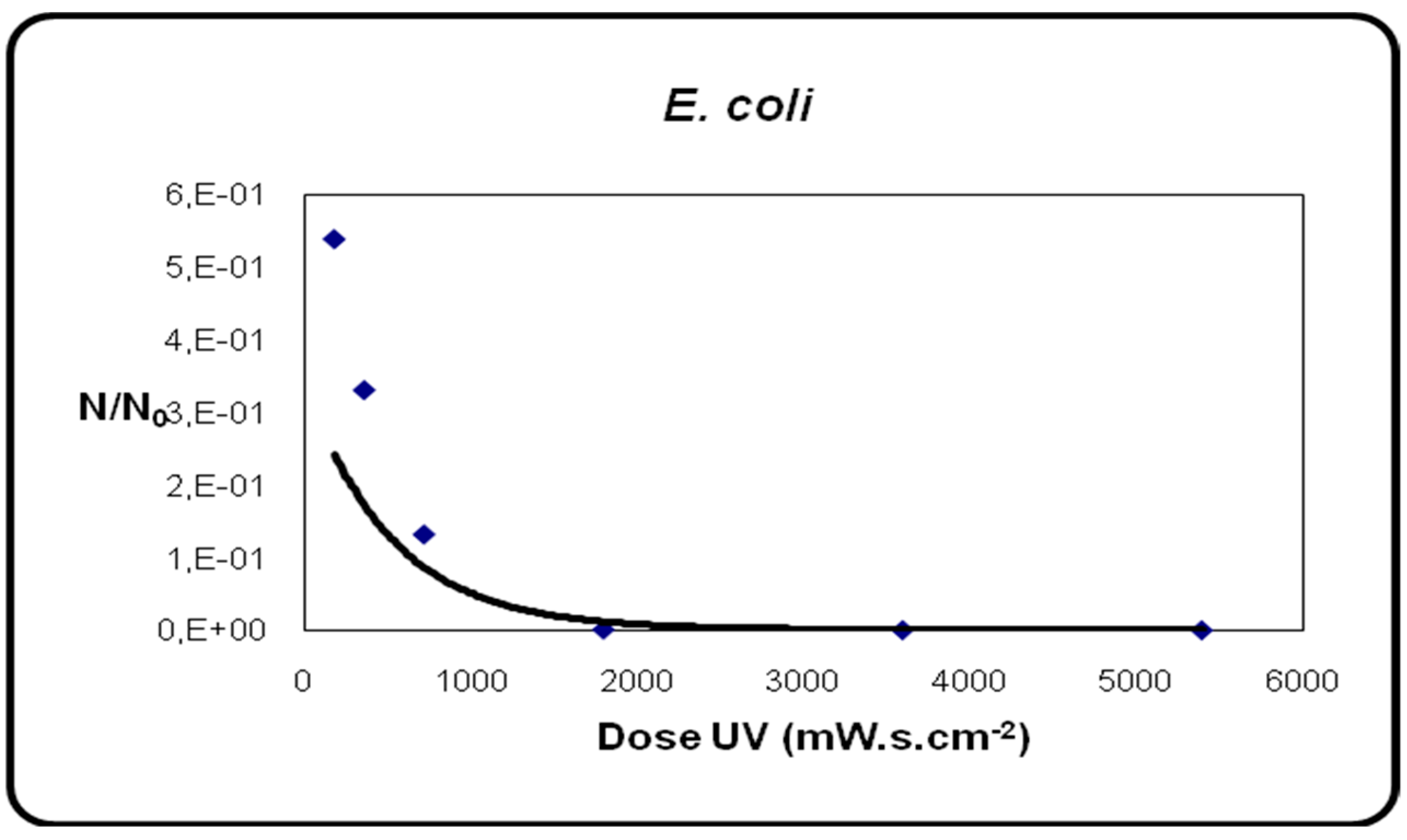
Simulations were generated by the combination of a PV generator with static converters, UV lamp and motor pump. The experimental results are very close to the simulations. This nuance is effectively taken into account by the simplifications introduced in the modeling process by averaging or ignoring the chopper losses and dissipation. However, despite this nuance, the new structure adopted is very useful and efficient, since it allows the creation of an autonomous water treatment system, ensuring better water quality. After verifying the controls implemented experimentally, we compared the kinetics of bacterial inactivation as a function of the dose of UV emitted by the discharge lamp during operation of the system in its new configuration, and to achieve the desired kinetics (desired water quality). Figure 47 shows the experimental and simulated curves of inactivation kinetics of Escherichia coli ATCC 29.
The image above clearly shows the efficiency of the new structure adopted and the controls implemented, which made it possible to create an autonomous water supply system while ensuring optimal water quality.
4. Conclusions
In this work, after studying the hardware configuration of the pilot water disinfection device, we analyzed the bacteriological results according to different flow rates and variable UV fluxes.
Any change in climatic factors will lead to a change in photovoltaic production, which in turn affects water quality. So, using smart technique based on deep learning was preferable.
We have proposed a deep learning-based approach to model water disinfection phenomena (phenomena that exhibit nonlinear relationships) because any change in climatic factors will lead to a change in photovoltaic production, which in turn affects water quality. This method makes it possible to estimate the parameter adapted to each load, i.e., motor-pump and UV lamps. The advantage of this approach is to guarantee better water quality in real time according to the energy available. The control of the other parts of the system (DC/DC converter, inverter, electric pump) was also studied. These different control modes were implemented in real time. This experimental validation was carried out to reinforce the simulation results and especially to prove the effectiveness of the various control techniques used.
Author Contributions
This article was written by N.Z., R.G., R.A. and D.M. All authors have read and agreed to the published version of the manuscript.
Funding
The authors received no financial support for the research, authorship and/or publication of this article.
Data Availability Statement
Not applicable.
Acknowledgments
The hardware was used and the results obtained in the research unit ERCO INSAT, Tunisia, and the research center CRTE. All the authors mentioned in this work have already given permission to submit this work.
Conflicts of Interest
The authors declared no potential conflict of interest with respect to the research, authorship and/or publication of this article.
References
- Gammoudi, R.; Brahmi, H.; Dhifaoui, R. Estimation of Climatic Parameters of a PV System Based on Gradient Method. Complexity 2019, 2019, 7385927. [Google Scholar] [CrossRef]
- Alayi, R.; Sevbitov, A.; Assad, M.E.H. Investigation of energy and economic parameters of photovoltaic cells in terms of different tracking technologies. Int. J. Low-Carbon Technol. 2022, 17, 160–168. [Google Scholar] [CrossRef]
- Almallahi, M.N.; Assad, M.E.H.; Alshihabi, S.; Alayi, R. Multi-criteria decision-making approach for the selection of cleaning method of solar PV panels in United Arab Emirates based on sustainability perspective. Int. J. Low-Carbon Technol. 2022, 17, 380–393. [Google Scholar] [CrossRef]
- Gorji, S.A.; Ektesabi, M.; Zheng, J. Isolated switched-boost push-pull DC-DC converter for step-up applications. Electron. Lett. 2017, 53, 177–1796. [Google Scholar] [CrossRef]
- Hemza, A.; Abdeslam, H.; Chenni, R.; Narimene, D. Photovoltaic system output simulation under various environmental conditions. In Proceedings of the 2016 International Renewable and Sustainable Energy Conference IRSEC, Marrakech, Morocco, 16–17 November 2016; pp. 722–726. [Google Scholar]
- AlShabi, M.; Ghenai, C.; Bettayeb, M.; Ahamad, F.F.; Assad, M.E.H. Multi-group grey wolf optimizer (MG-GWO) for estimating photovoltaic solar cell model. J. Therm. Anal. Calorim. 2021, 144, 1655–1670. [Google Scholar] [CrossRef]
- Carreño-Ortega, A.; Galdeano-Gómez, E.; Pérez-Mesa, J.C.; Del Galera-Quiles, M.C. Policy and environmental implications of photovoltaic systems in farming in southeast Spain: Can greenhouses reduce the greenhouse effect. Energies 2017, 10, 761. [Google Scholar] [CrossRef]
- Zitouni, N.; Gammoudi, R.; Hamrouni, N. An ANN–Constant power generation control for LVRT of grid-connected PVG. Energy Explor. Exploit. SAGE J. 2022, 41, 1150528. [Google Scholar] [CrossRef]
- Balamurugan, T.; Manoharan, S.; Sheeba, P.; Hafaifa, A. design a photovoltaic array with boost converter using fuzzy logic controller. Int. J. Electr. Eng. Technol. 2012, 3, 444–456. [Google Scholar]
- Ralik, A.; Jusoh, A.; Sutikno, T. A review on perturb and observe maximum power point tracking in photovoltaic system. Indones. J. Electr. Eng. Comput. Sci. 2015, 13, 745–751. [Google Scholar]
- Li, C.; Chen, Y.; Zhou, D.; Liu, J.; Zeng, J. A high-performance adaptive incremental conductance MPPT algorithm for photovoltaic systems. Energies 2016, 9, 288. [Google Scholar] [CrossRef]
- Bao, X.; Tan, P.; Zhuo, F.; Yue, X. Low voltage ride through control strategy for high-power grid-connected photovoltaic inverter. In Proceeding of the 28th Conference on Applied Power Electronics Conference and Exposition (APEC), Long Beach, CA, USA, 17–21 March 2013; pp. 97–100. [Google Scholar]
- Hejri, M.; Mokhtari, H.; Azizian, M.R.; Ghandhari, M.; Soder, L. On the parameter extraction of a fiveparameter double-diode model of photovoltaic cells and modules. IEEE J. Photovolt. 2014, 4, 915–923. [Google Scholar] [CrossRef]
- Chu, Y.M.; Shankaralingappa, B.M.; Gireesha, B.J.; Alzahrani, F.; Khan, M.; Khan, S.U. Combined impact of Cattaneo-Christov double diffusion and radiative heat flux on bio-convective flow of Maxwell liquid configured by a stretched nanomaterial surface. Appl. Math. Comput. 2022, 419, 126883. [Google Scholar] [CrossRef]
- Mares, O.P.; Badescu, M.V. A simple but accurate procedure for solving the five-parameter model. Energy Convers. Manag. 2015, 105, 139–148. [Google Scholar] [CrossRef]
- Allani, M.Y.; Mezghani, D.; Tadeo, F.; Mami, A. FPGA Implementation of a Robust MPPT of a Photovoltaic System Using a Fuzzy Logic Controller Based on Incremental and Conductance Algorithm. Eng. Technol. Appl. Sci. Res. 2019, 9, 4322–4328. [Google Scholar] [CrossRef]
- Zissis, G.; Damelincourt, J.J.; Bezanahary, T. Modelling discharge lamps for electronic circuit designers: A review of the existing methods. IEEE Ind. Appl. Soc. 2001, 2, 1260–1262. [Google Scholar]
- Silva, E.A.; Bradaschia, F.; Cavalcanti, M.C.; Nascimento, A.J. Parameter estimation method to improve the accuracy of photovoltaic electrical model. IEEE J. Photovolt. 2016, 6, 278–285. [Google Scholar] [CrossRef]
- Labidi, Z.R.; Schulte, H.; Mami, A. A Model-Based Approach of DC-DC Converters Dedicated to Controller Design Applications for Photovoltaic Generators. Eng. Technol. Appl. Sci. Res. 2019, 9, 4371–4376. [Google Scholar] [CrossRef]
- Huang, M.; Ma, Y.; Wan, J.; Wang, Y. Simulation of a paper mill wastewater treatment using a fuzzy neural network. Expert Syst. Appl. 2009, 36, 5064–5070. [Google Scholar]
- Andoulsi, R.; Mami, A.; Dauphin-Tanguy, G.; Annabi, M. Modelling and simulation by bond graph technique of a DC motor fed from a photovoltaic source via MPPT boost converter. In Proceedings of the Conference of Particle Accelerator (CSSC’99), New York, NY, USA, 16–19 March 1987; pp. 4181–4187. [Google Scholar]
- Zitouni, N.; Gammoudi, R. Database for control a complex water treatment system powered by photovoltaic generator for deep learning. In Proceedings of the International Conference on Electrical, Computer and Energy Technologies (ICECET 2022), Prague, Czech Republic, 20–22 July 2022. [Google Scholar]
- Maged, M.H.; Khalafallah, M.G.; Hassanien, E.A. Prediction of wastewater treatment plant performance using artificial neural networks. Environ. Model. Softw. 2004, 19, 919–928. [Google Scholar]
Figure 1.
Schematic block of water treatment system.
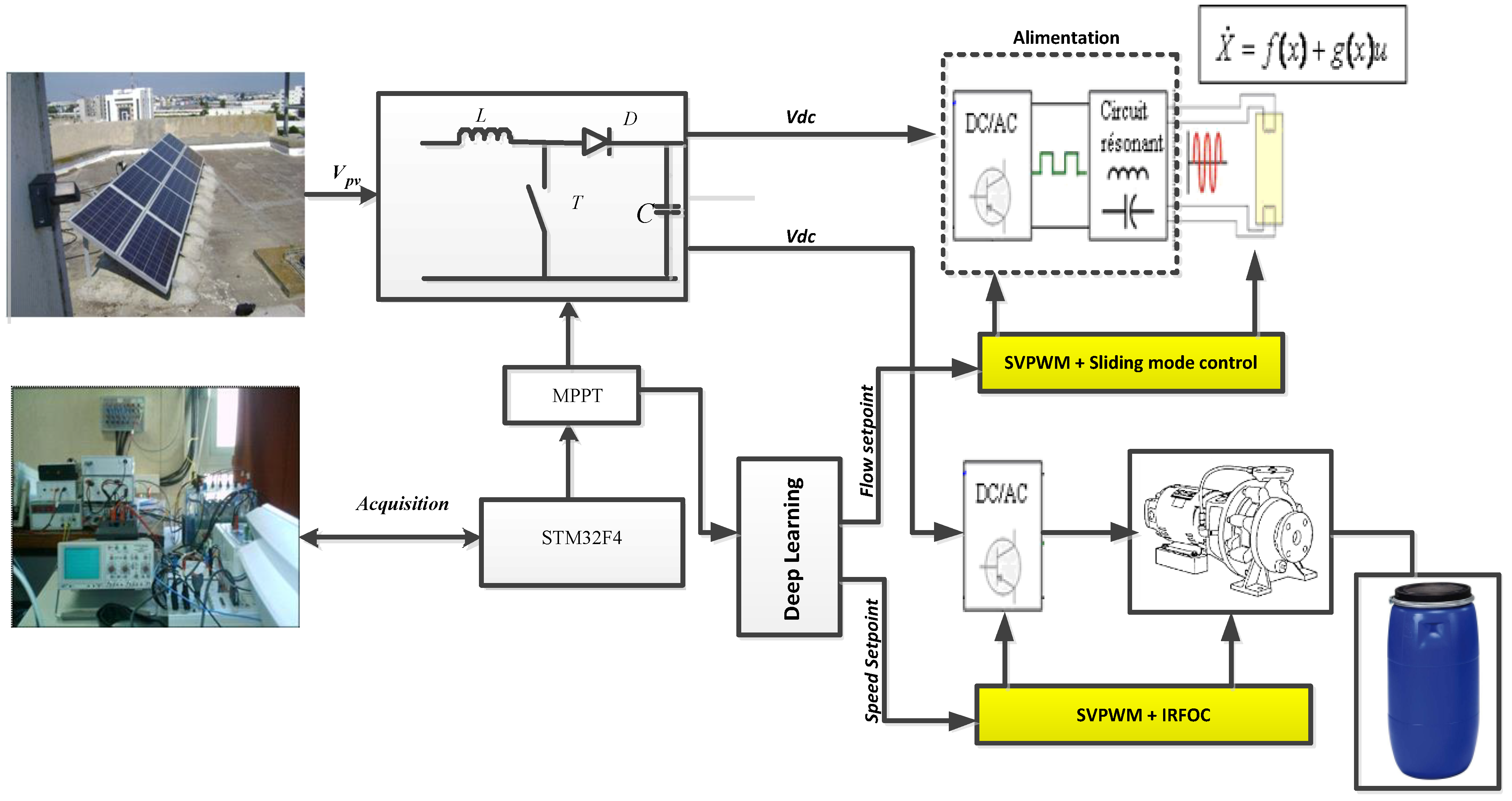
Figure 2.
One-diode model of PV cell.
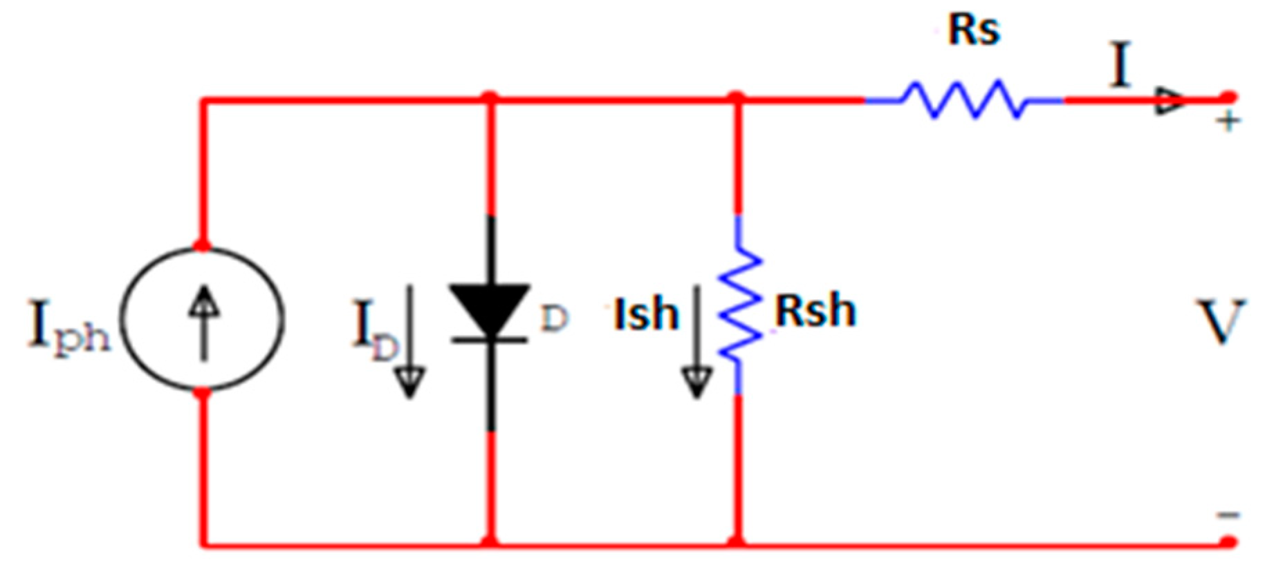
Figure 3.
Recording of GPV current and voltage quantities.
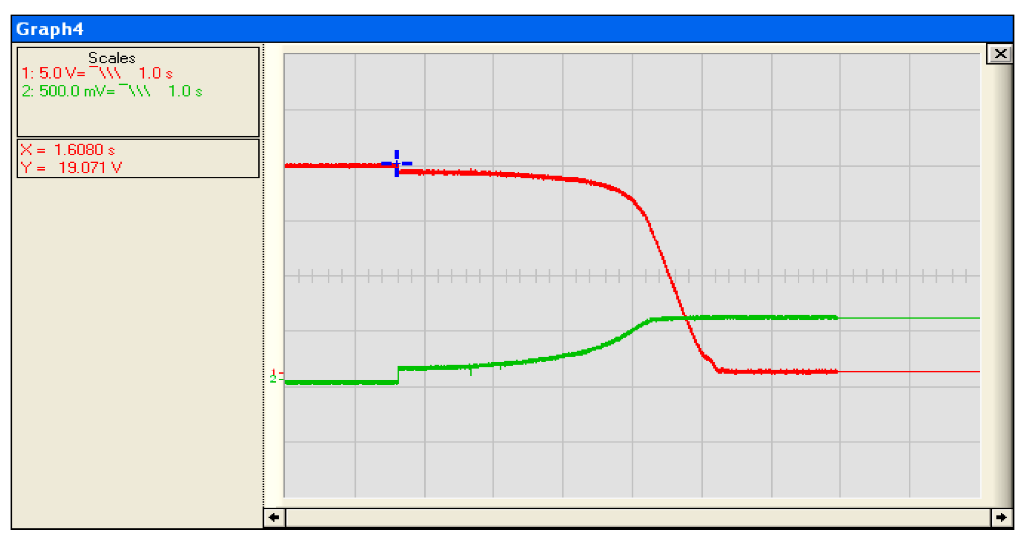
Figure 4.
I–V characteristics.
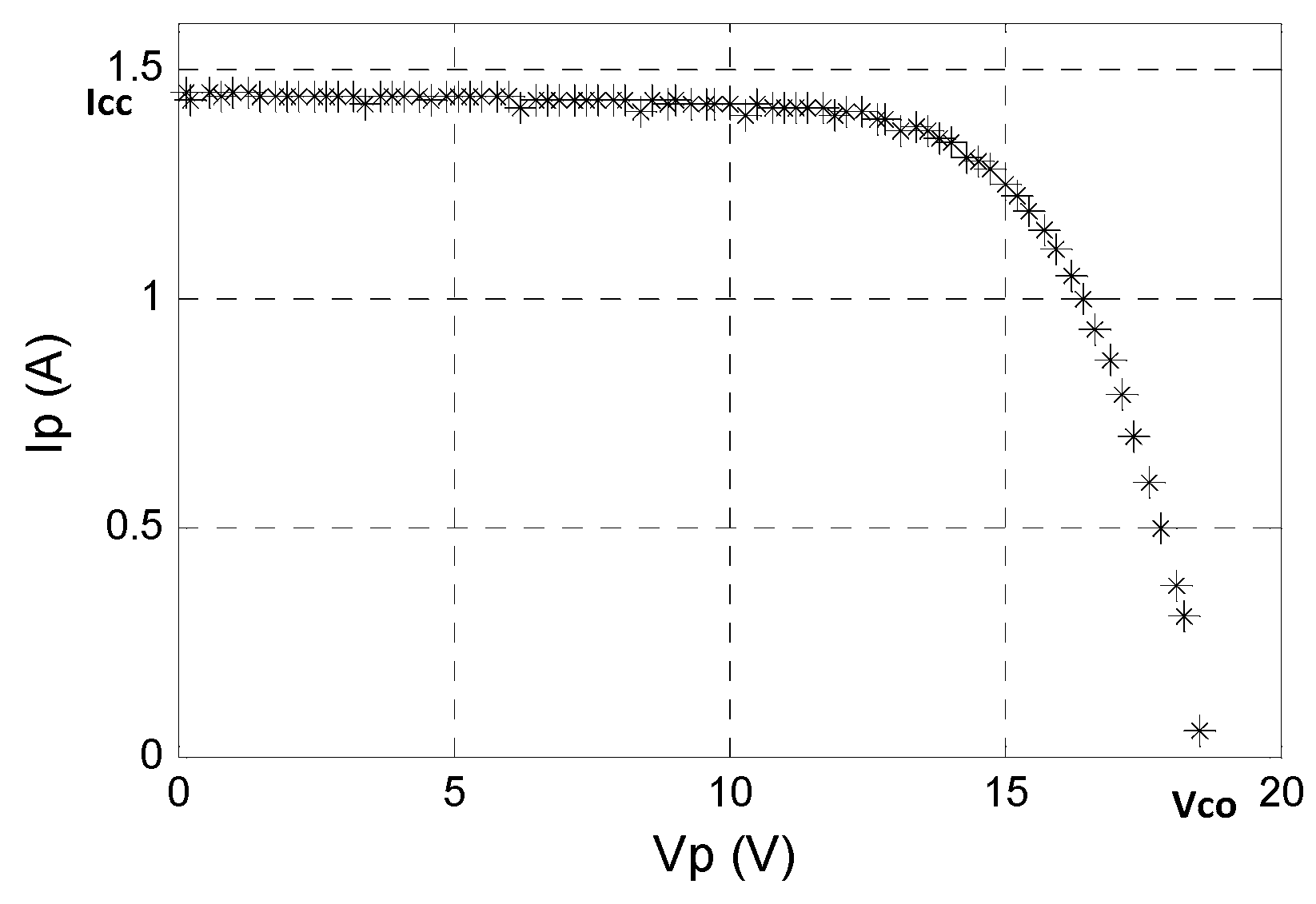
Figure 5.
Effects of Rs and Rsh resistances.
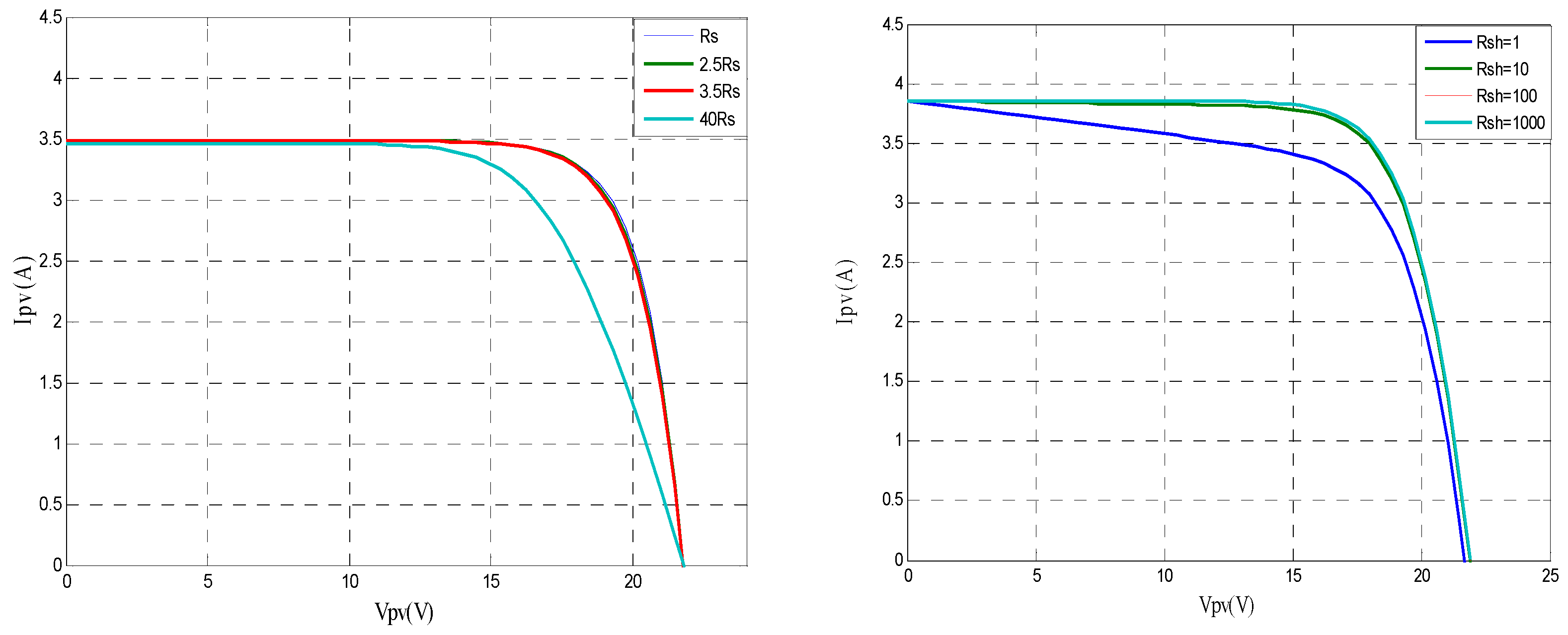
Figure 6.
Influence of illumination on series resistance.
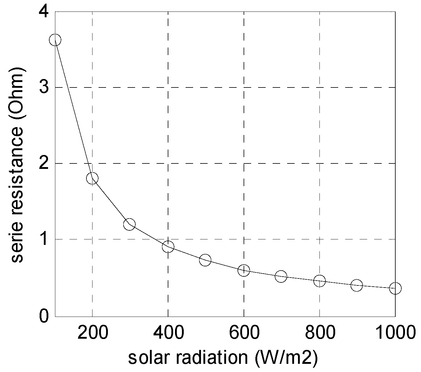
Figure 7.
Influence of junction temperature on series resistance.
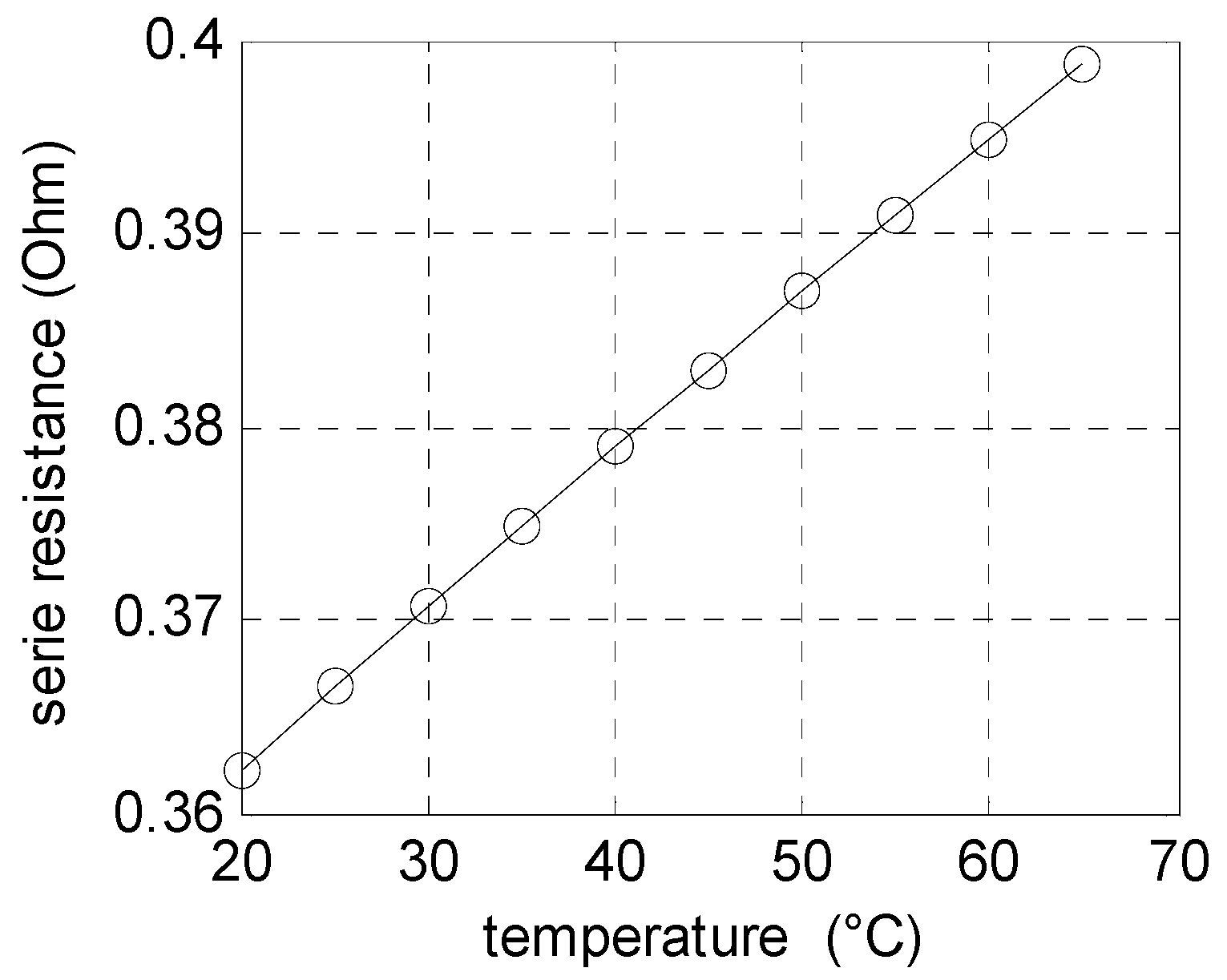
Figure 8.
Influence of illumination on shunt resistance.
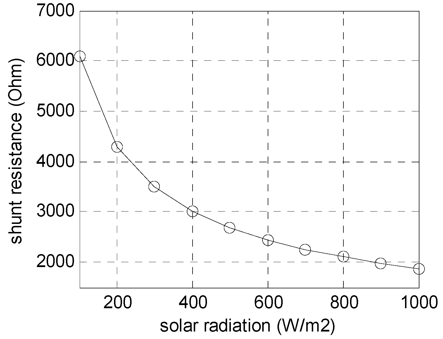
Figure 9.
Influence of junction temperature on shunt resistance.
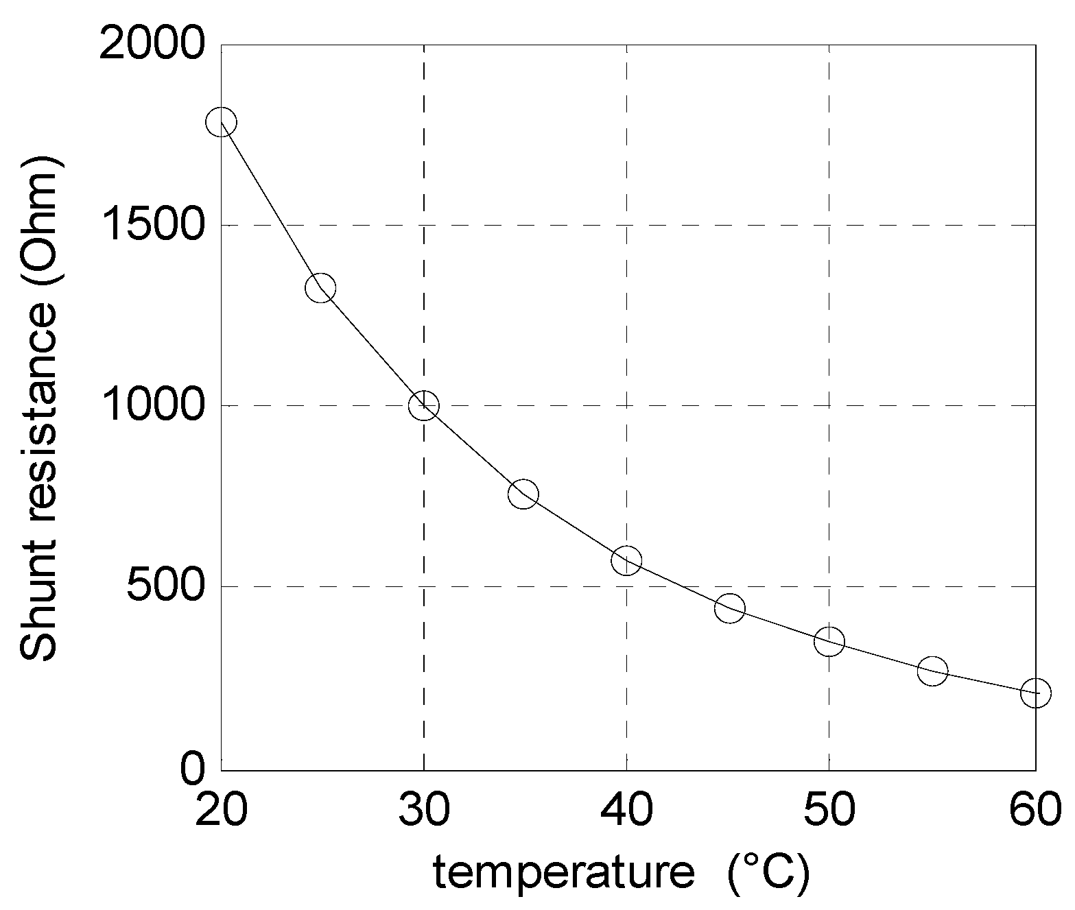
Figure 10.
Illumination effect.
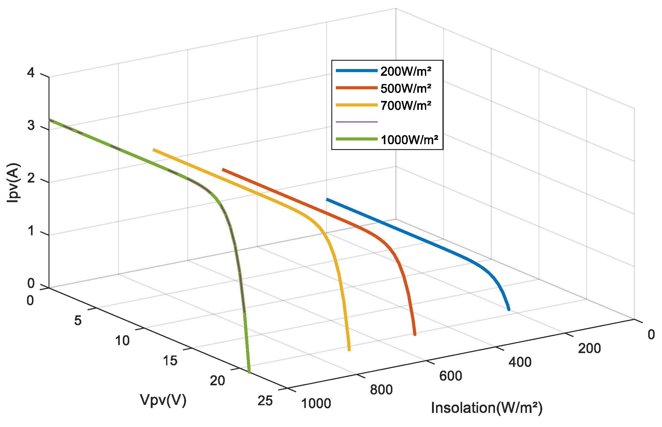
Figure 11.
Temperature effect.
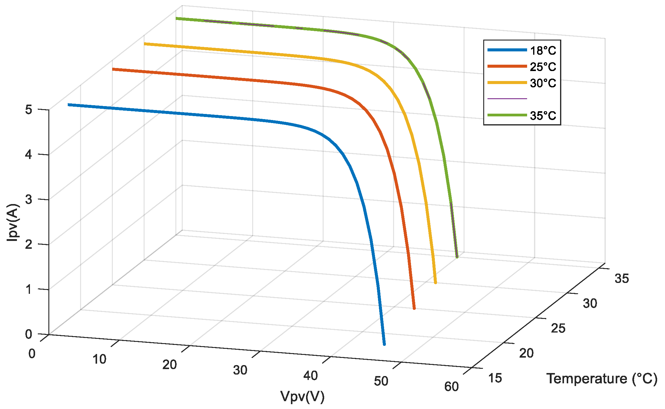
Figure 12.
Booster chopper.

Figure 13.
Different convergence modes for trajectory state.

Figure 14.
Equivalent wiring diagram of power supply UV lamp A.
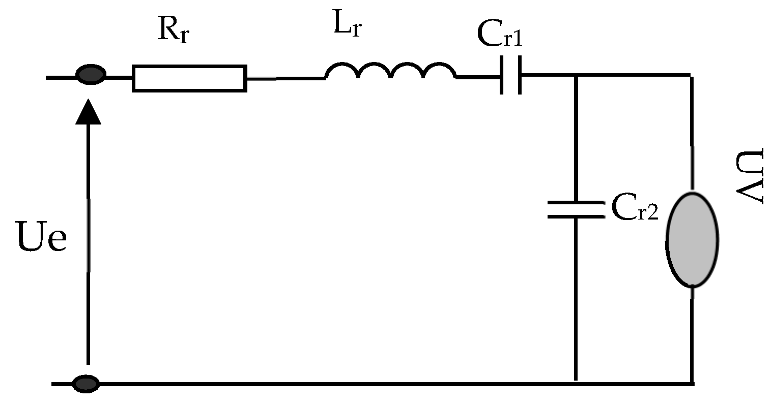
Figure 15.
New system operation structure.
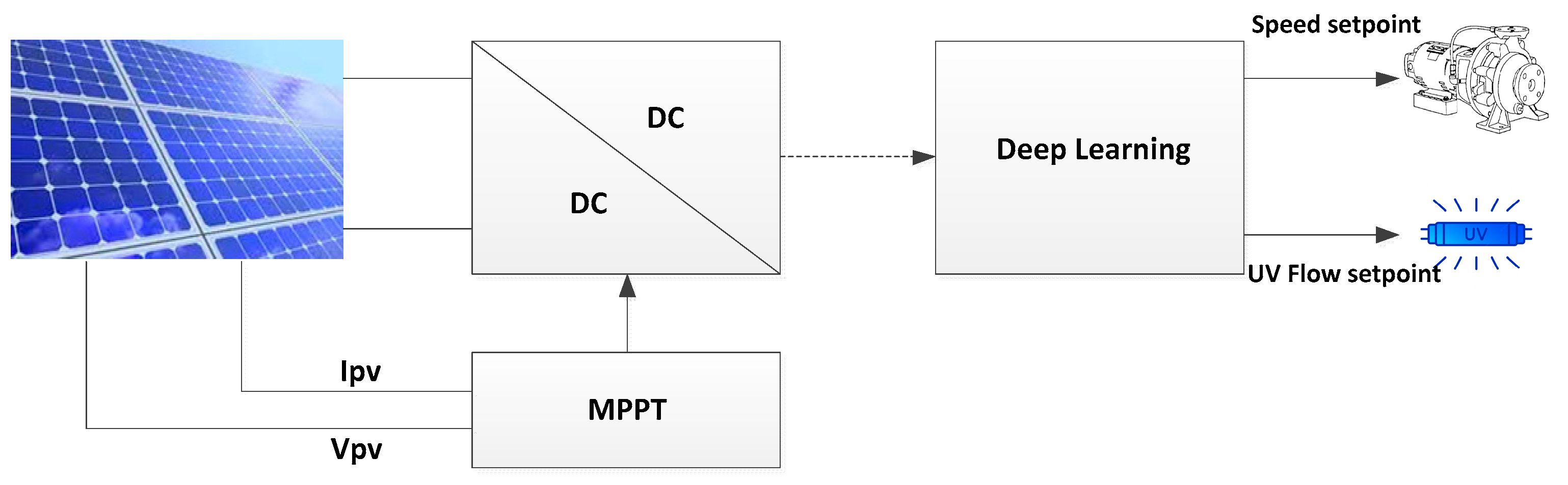
Figure 16.
Schematic model of the UV water disinfection system.
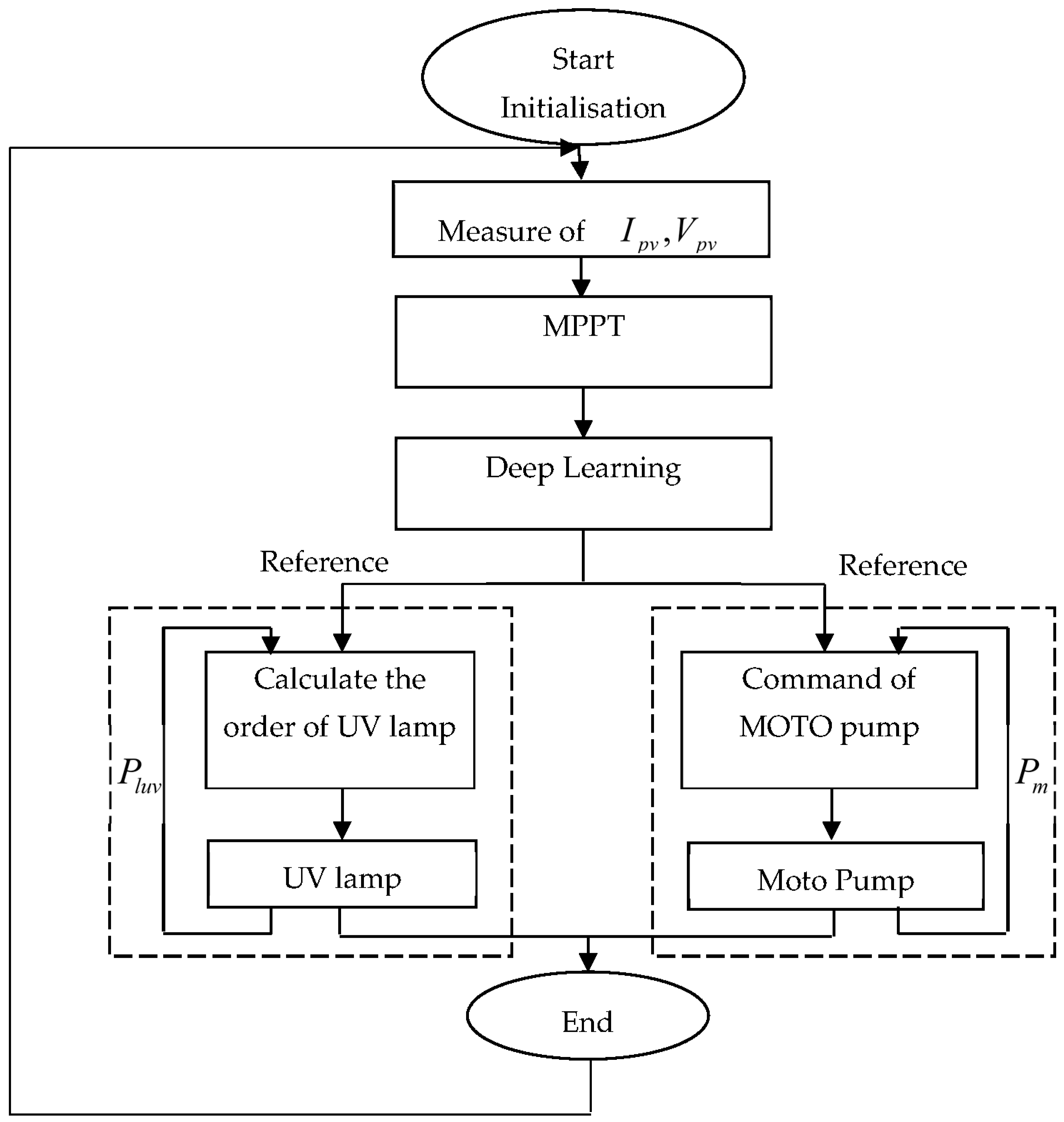
Figure 17.
Block diagram of three-phase inverter.
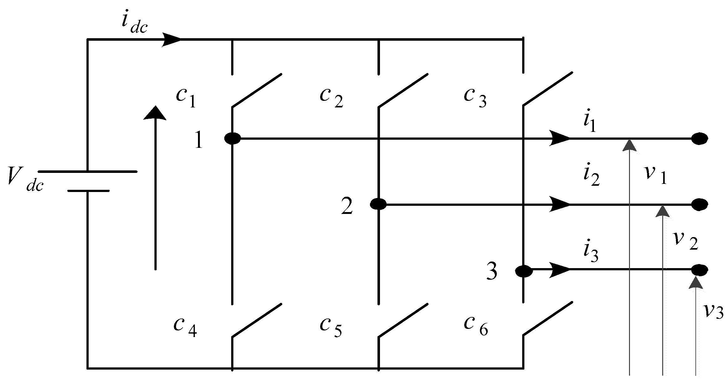
Figure 18.
Synthesis of the SVPWM technique.
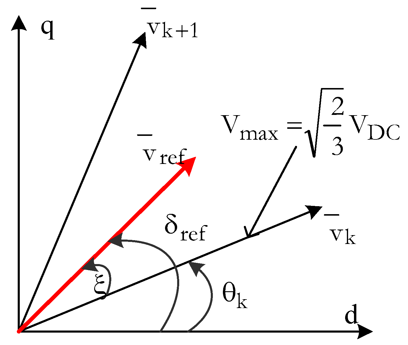
Figure 19.
Photovoltaic pumping system with sliding mode vector control.
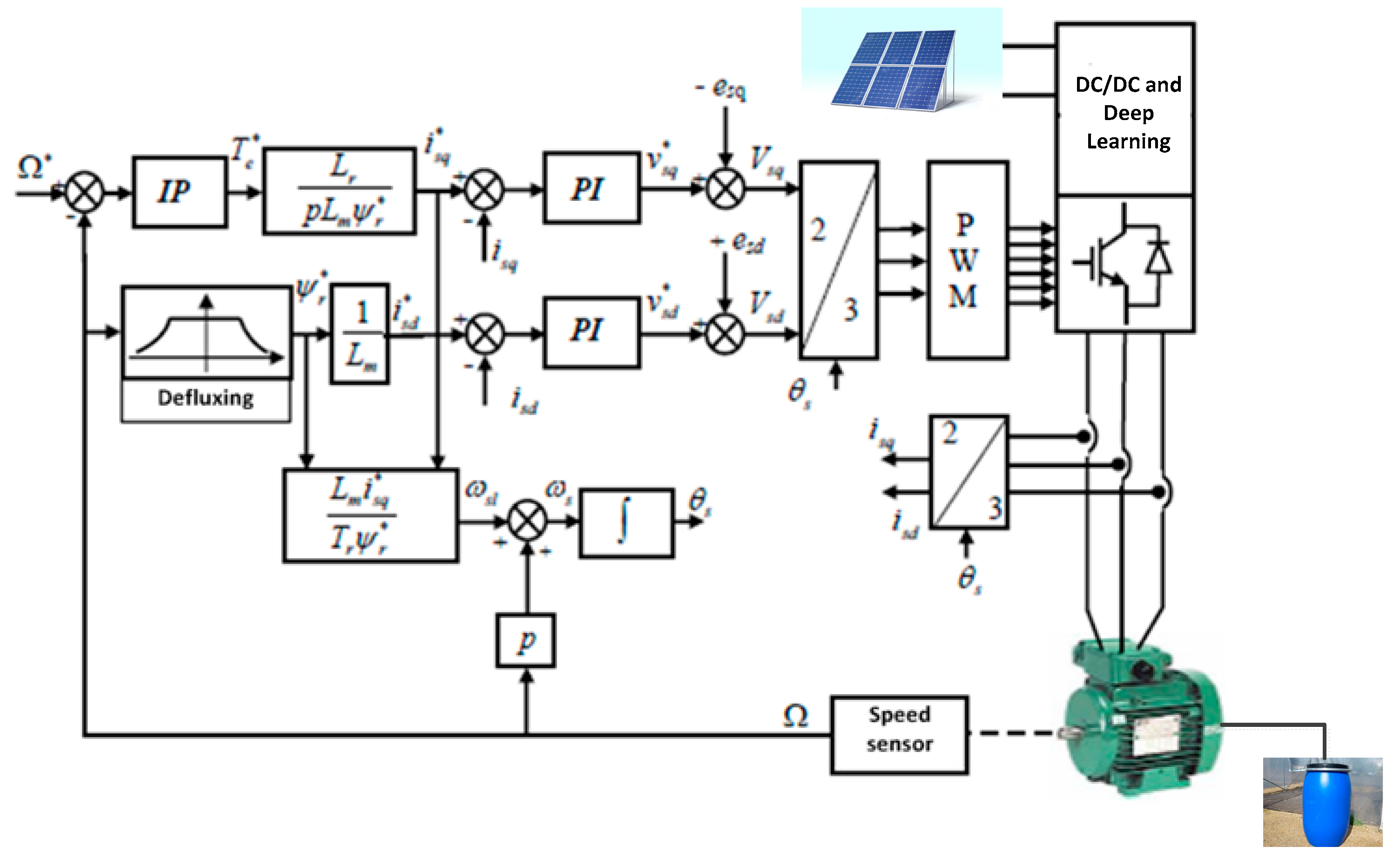
Figure 20.
Equivalent electrical diagram of UV lamp power supply.

Figure 21.
Simulation of UV lamp power with α = 0.9 (a), α = 0.5 (b).
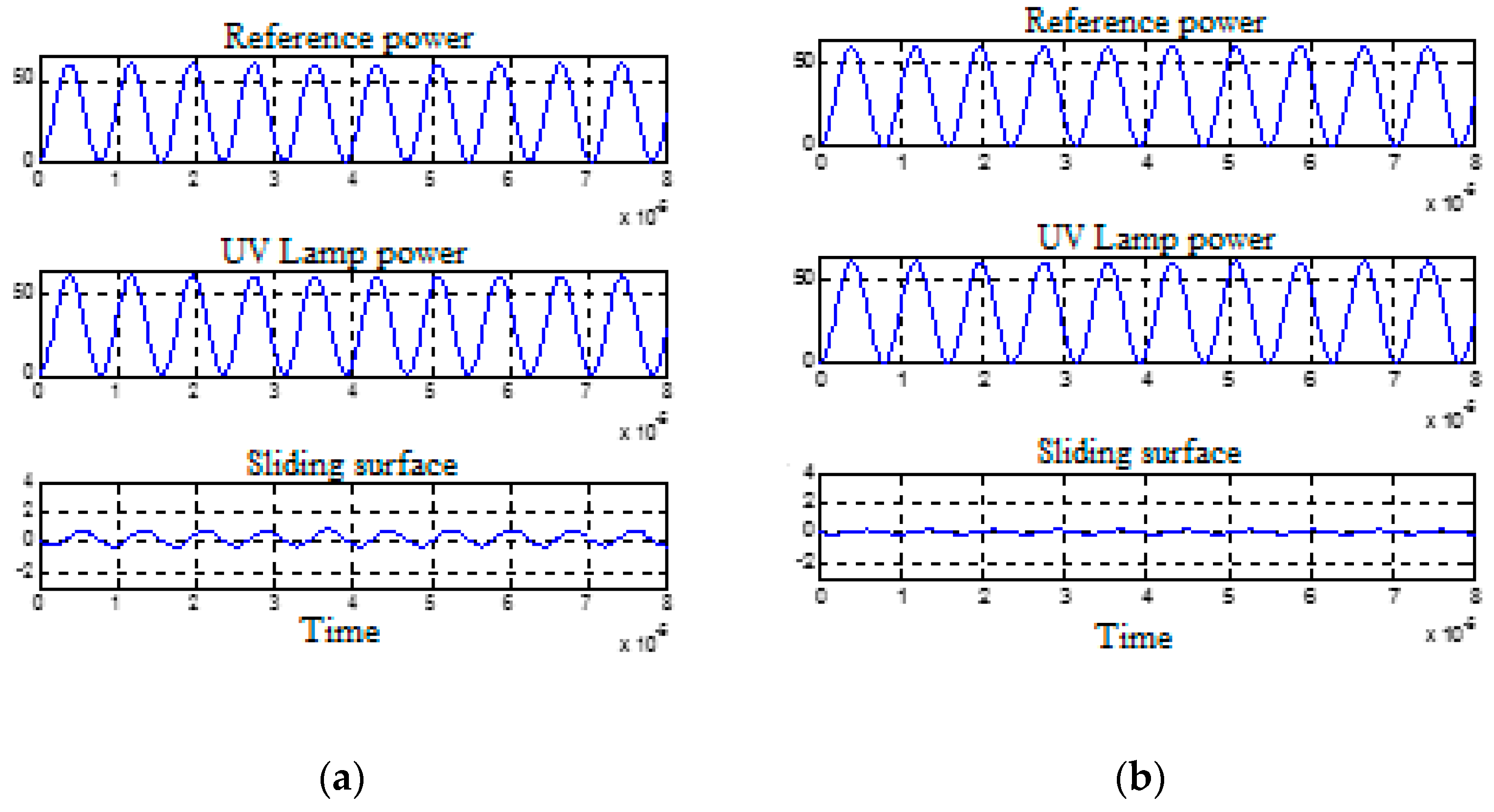
Figure 22.
Simulated UV lamp power with α = 0.9, 90% change in inductance .
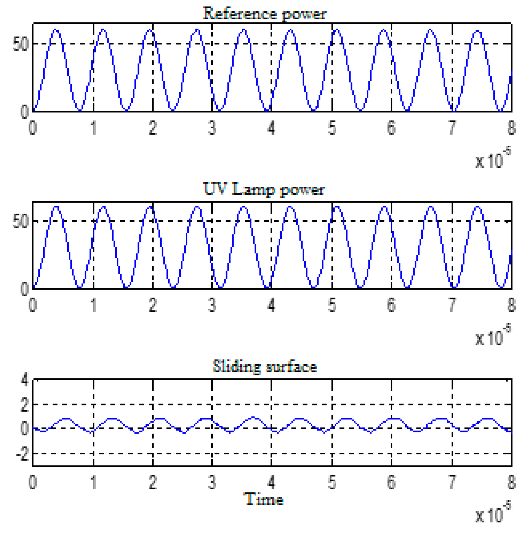
Figure 23.
General view of test bench.
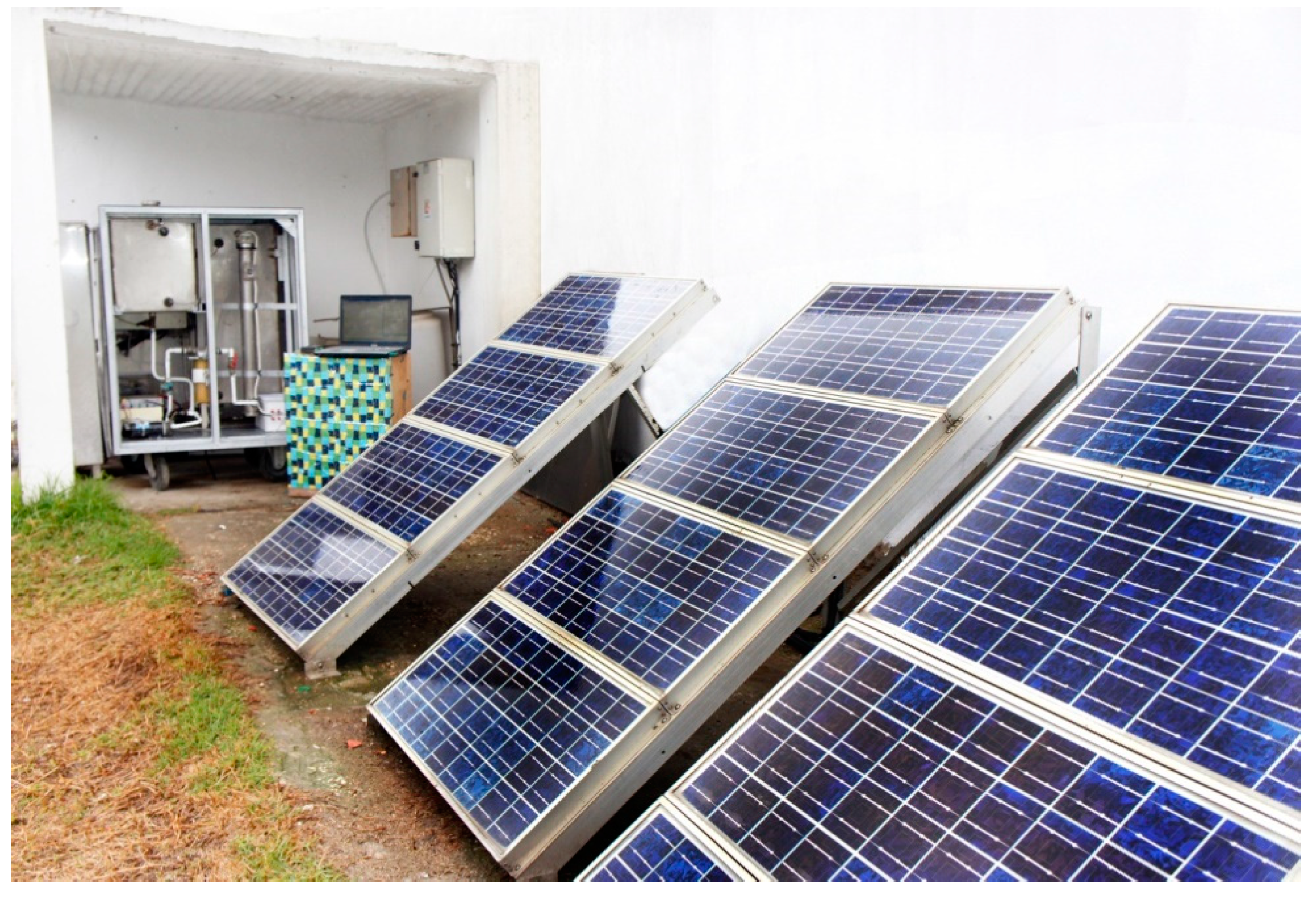
Figure 24.
General structure of the test bench (MPPT part).
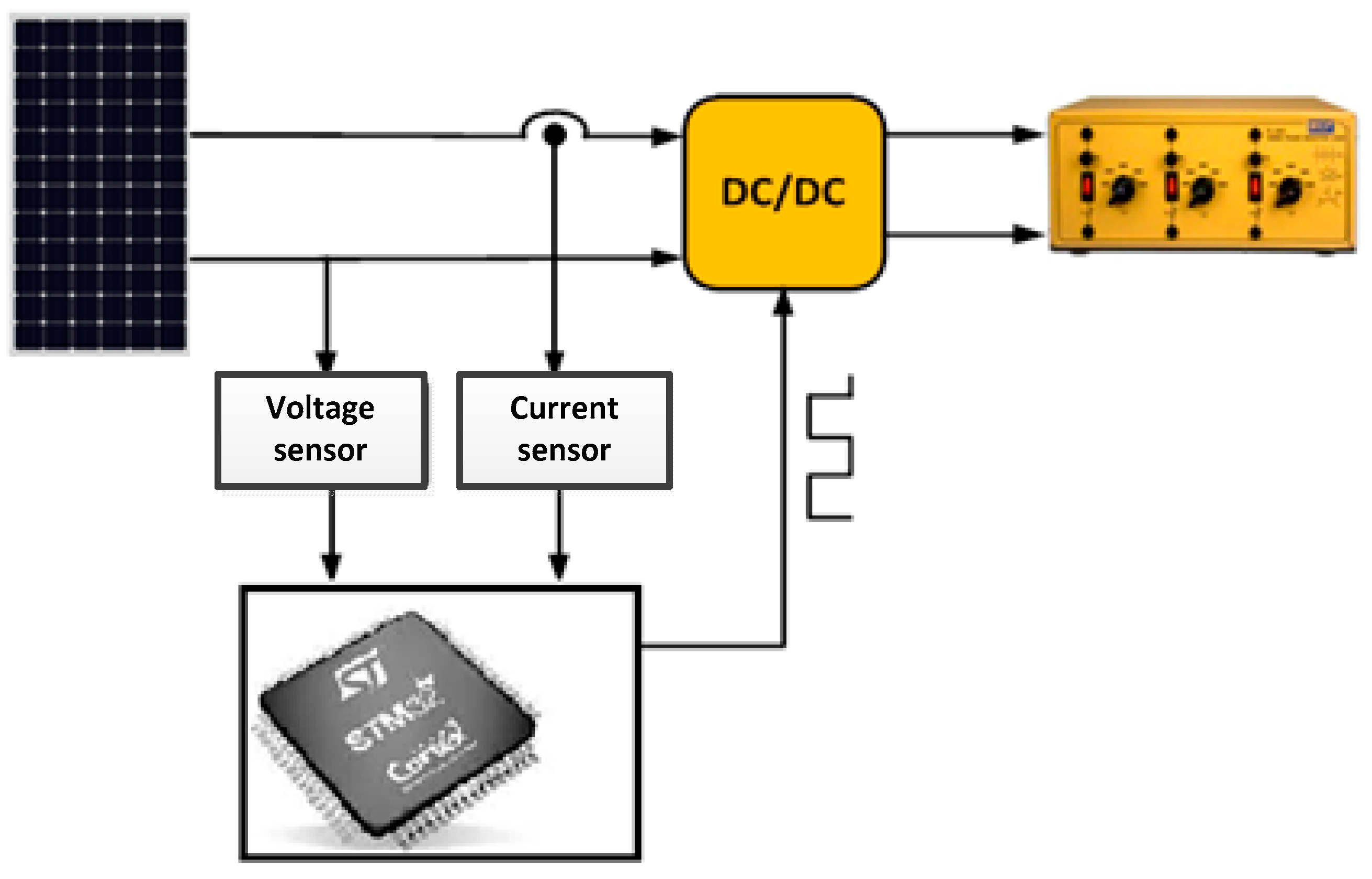
Figure 25.
Statement of Vpv, Ipv, Ins and temperature.

Figure 26.
Evolution of insolation.
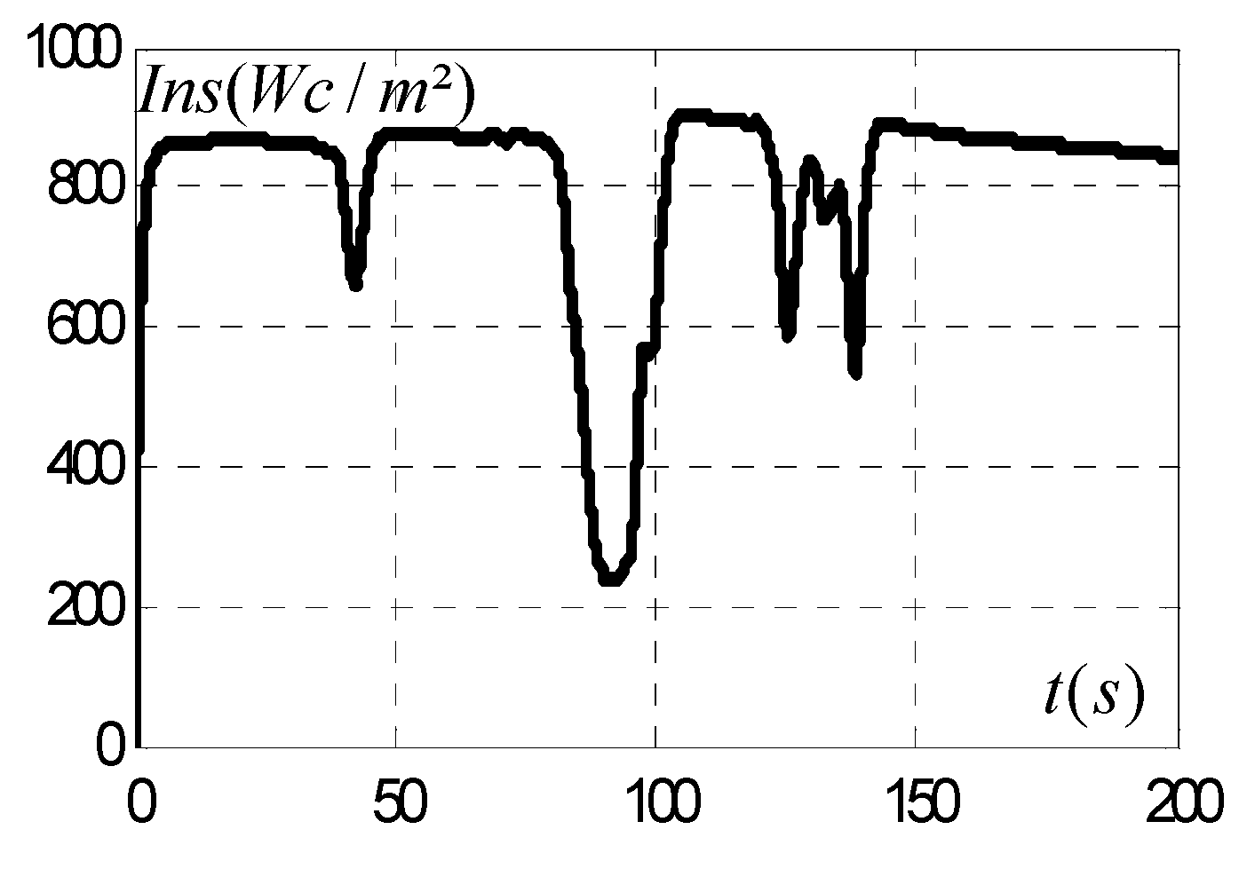
Figure 27.
Evolution of temperature.
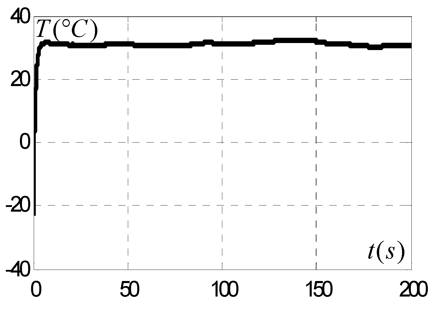
Figure 28.
Power variation.
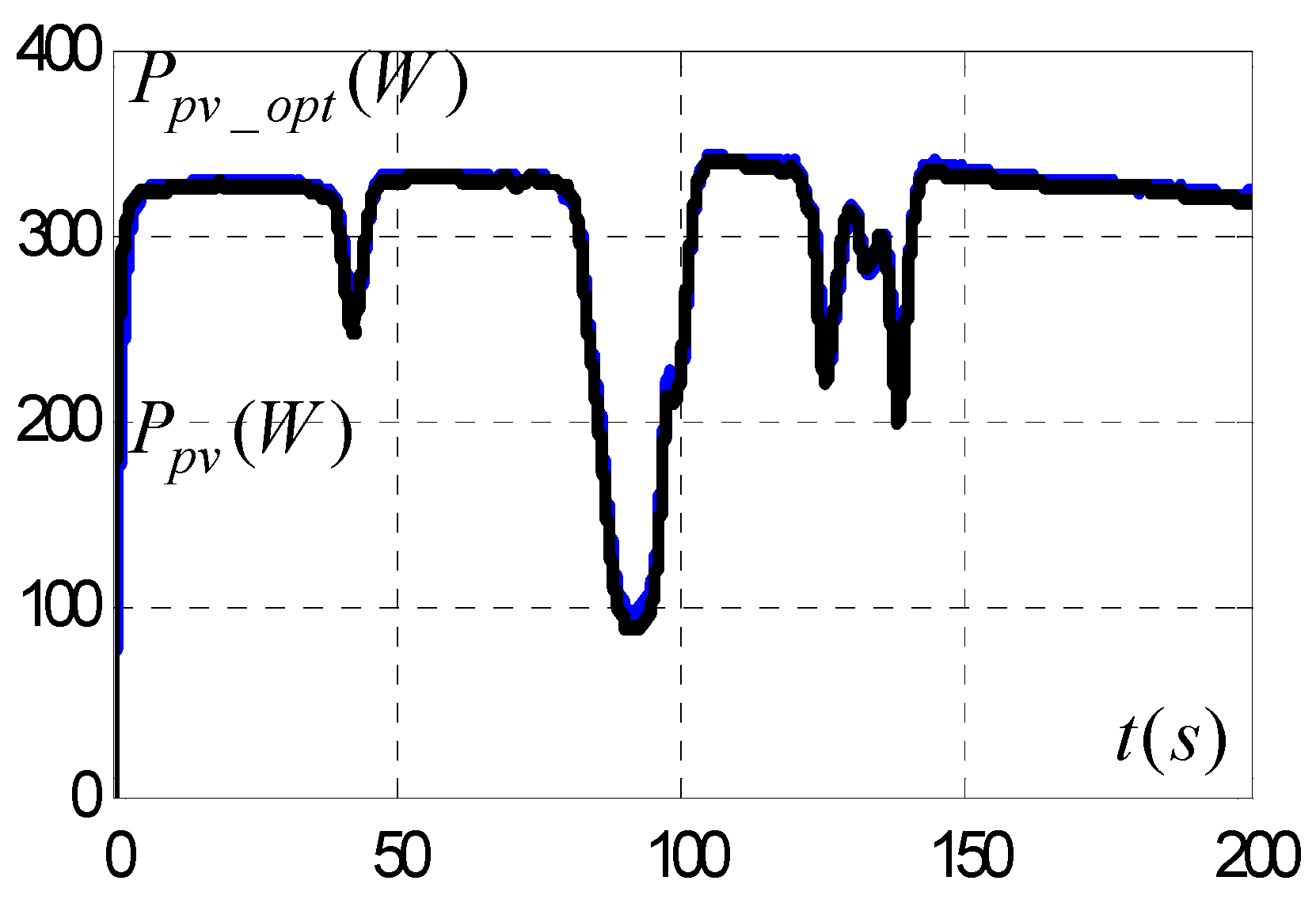
Figure 29.
Trajectory of MPP.
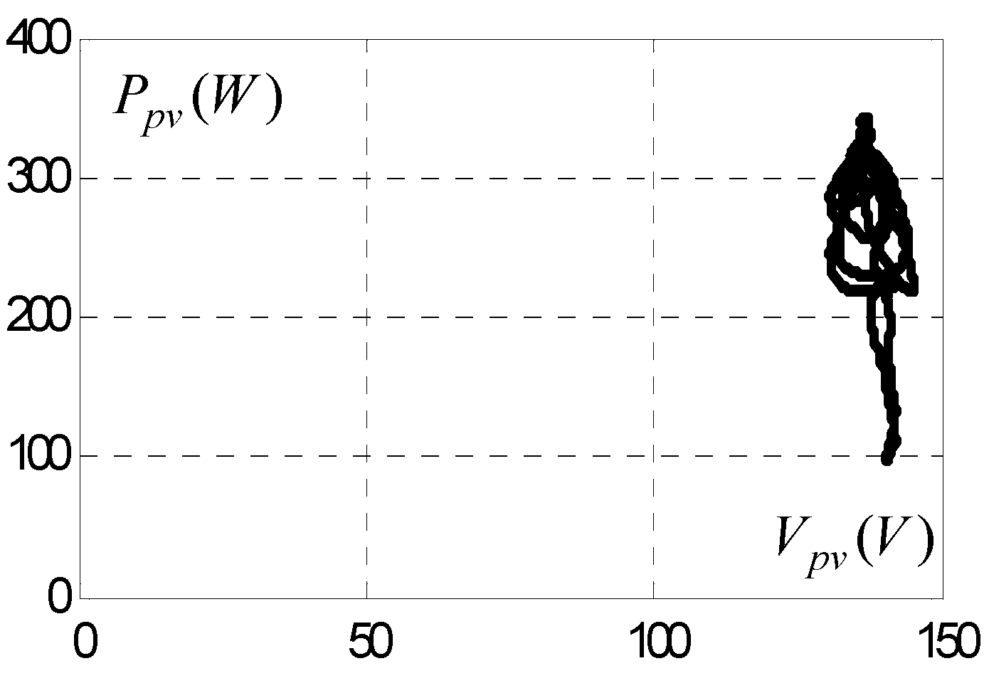
Figure 30.
Zoom of the displacement of MPP.

Figure 31.
Trajectory of MPP.
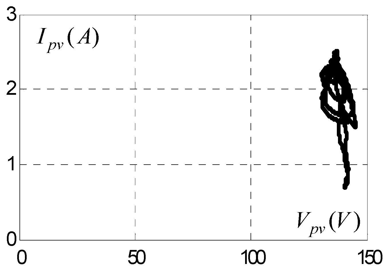
Figure 32.
Zoom of the displacement of MPP.

Figure 33.
Direct and quadrature voltage components.
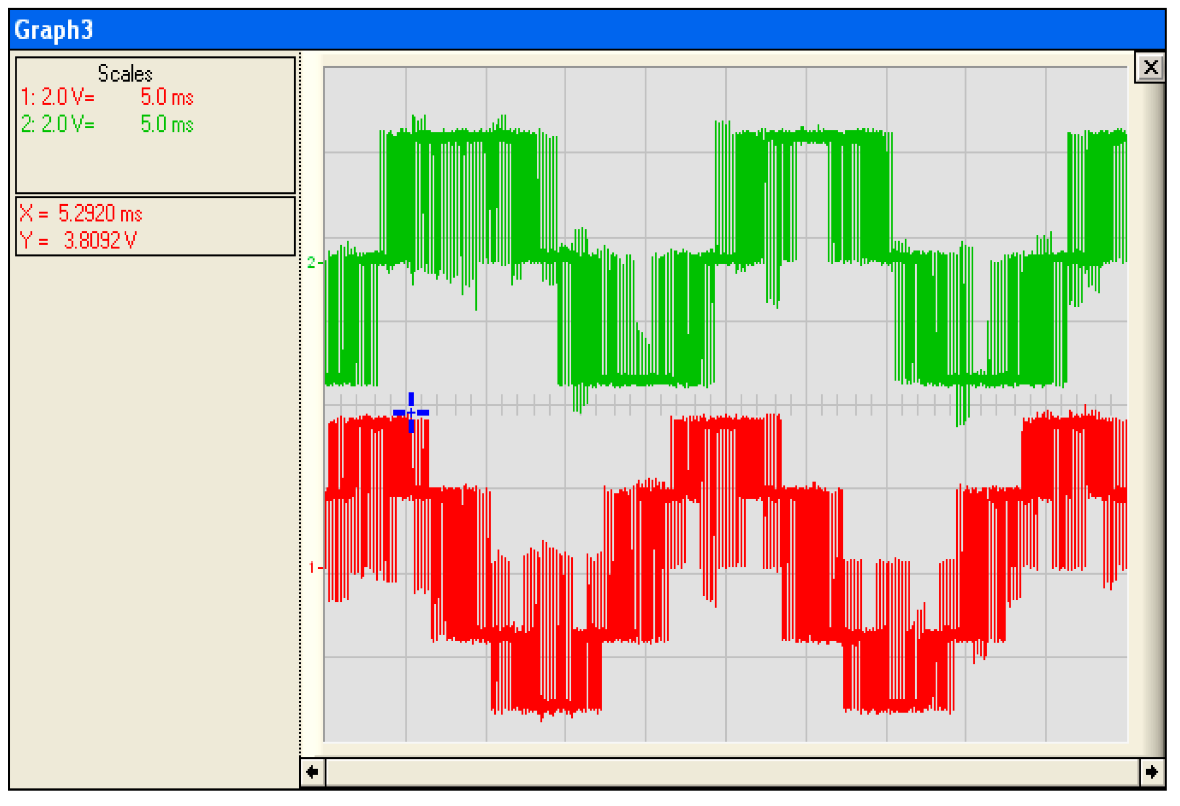
Figure 34.
The control signals generated by the interface board (15 V).
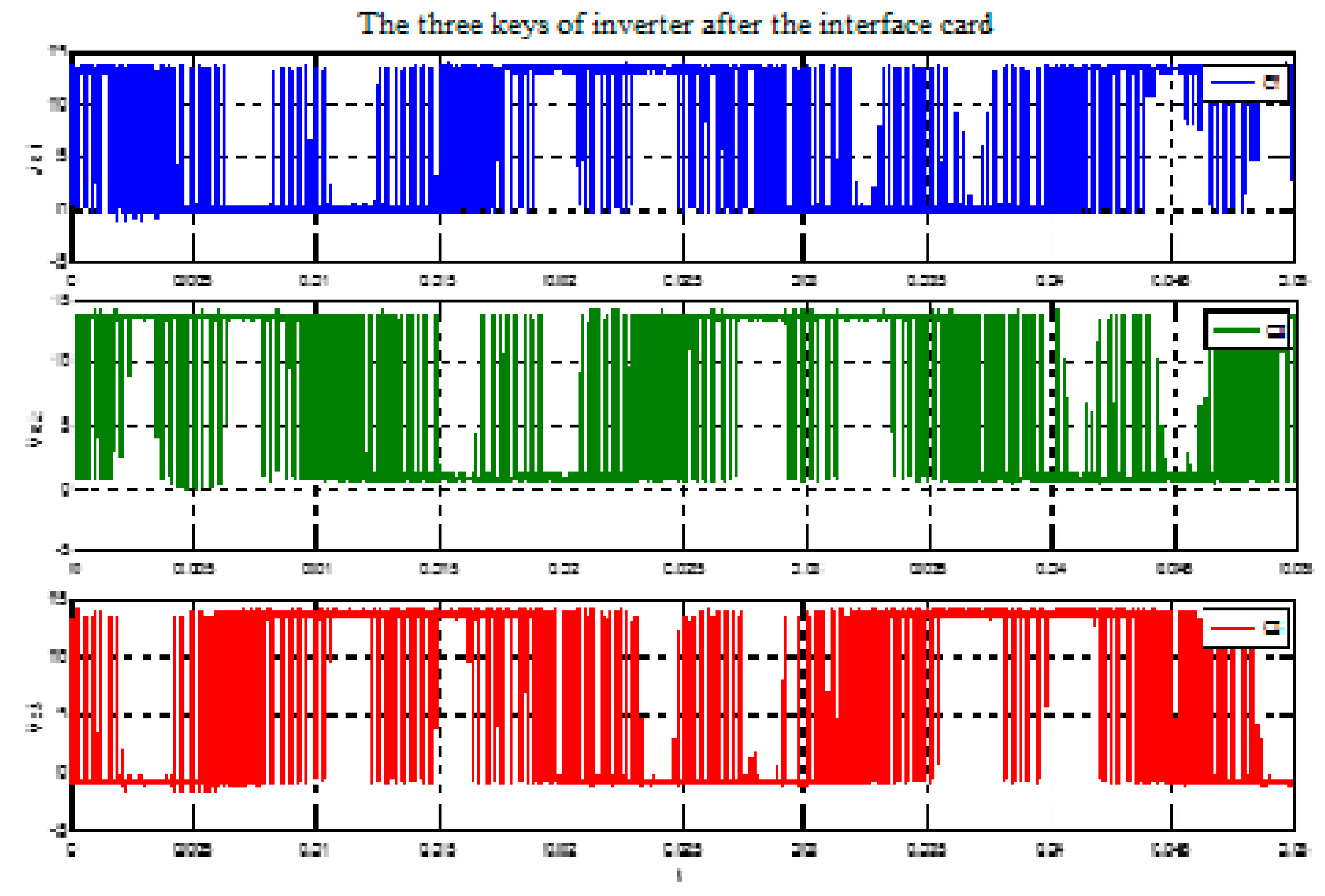
Figure 35.
Unfiltered direct and quadrature voltage component.
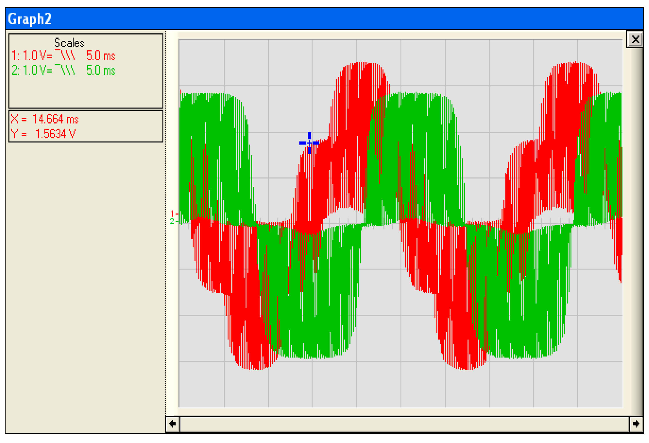
Figure 36.
Filtered direct and quadrature voltage component.
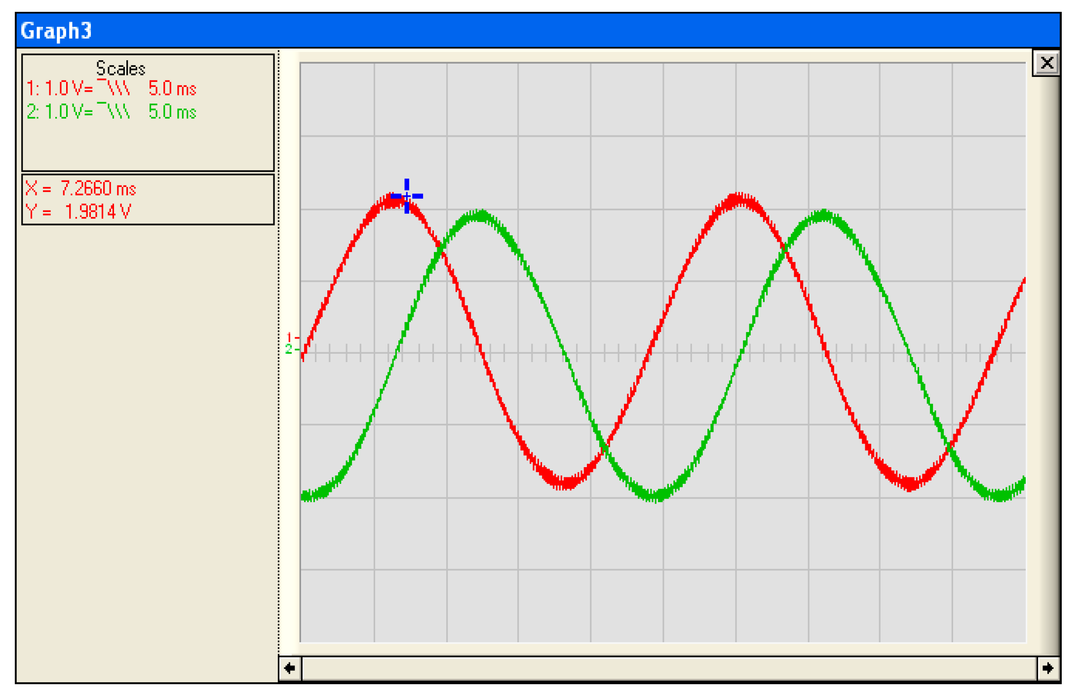
Figure 37.
Unfiltered Vd = f(Vq).

Figure 38.
.
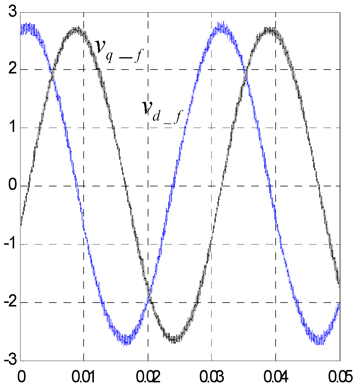
Figure 39.
.

Figure 40.
Variation of the angular speed and its reference.
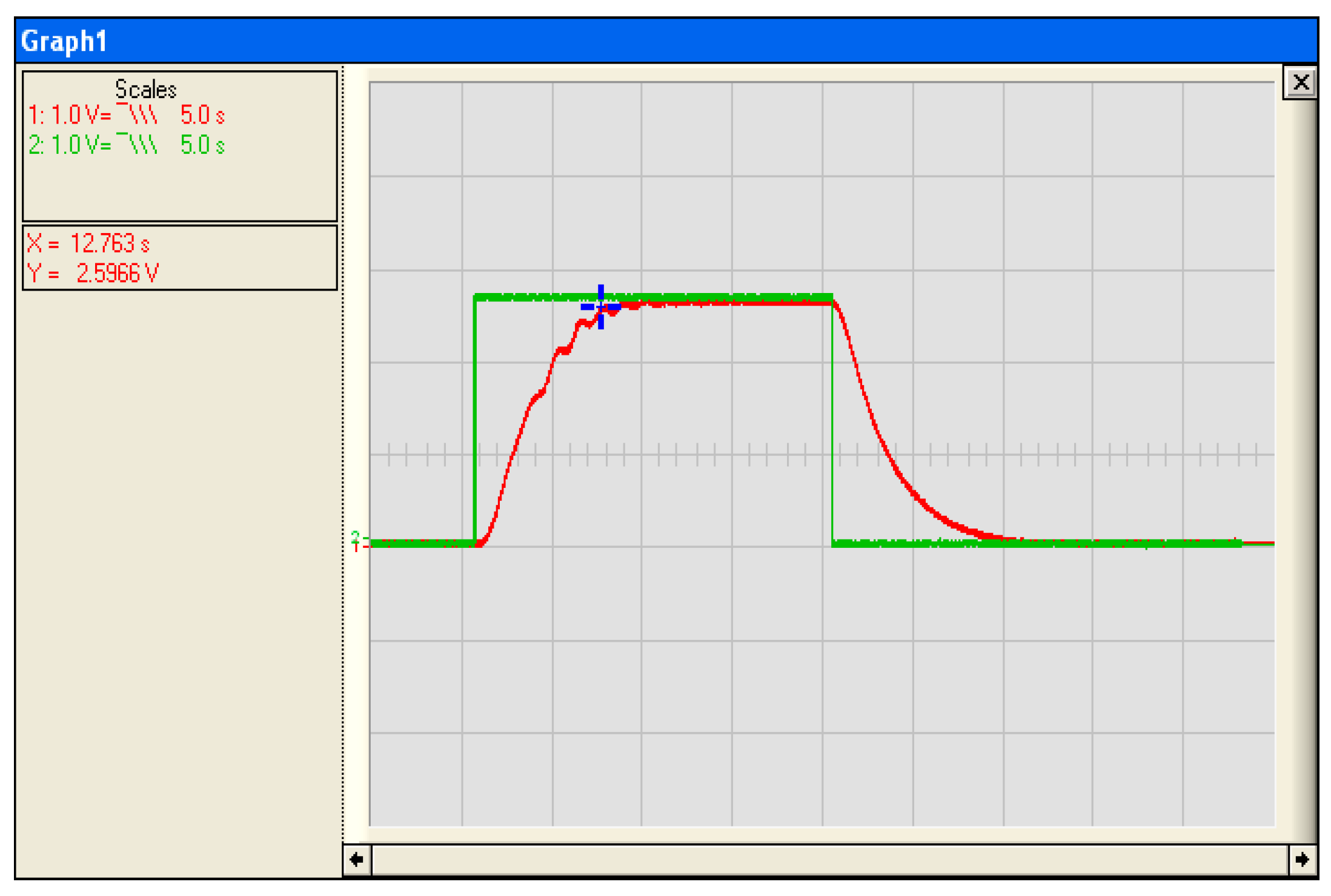
Figure 41.
Development of lighting, reference power for photovoltaic generators and reference voltage for GPV.
Figure 41.
Development of lighting, reference power for photovoltaic generators and reference voltage for GPV.
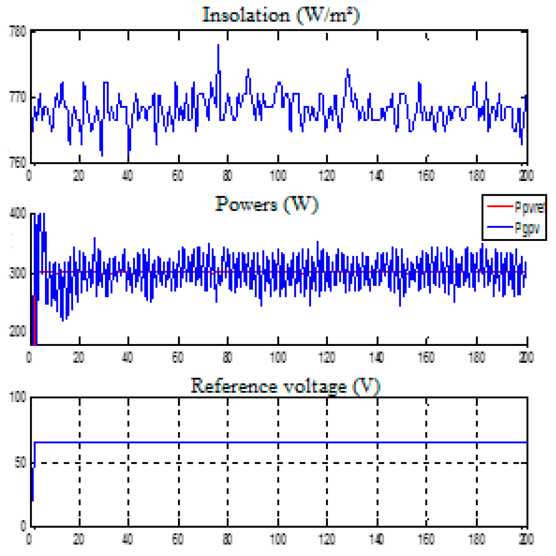
Figure 42.
Development of control law, power of UV lamp, input voltage of DC/DC converter () and input current of DC/DC converter ().
Figure 42.
Development of control law, power of UV lamp, input voltage of DC/DC converter () and input current of DC/DC converter ().
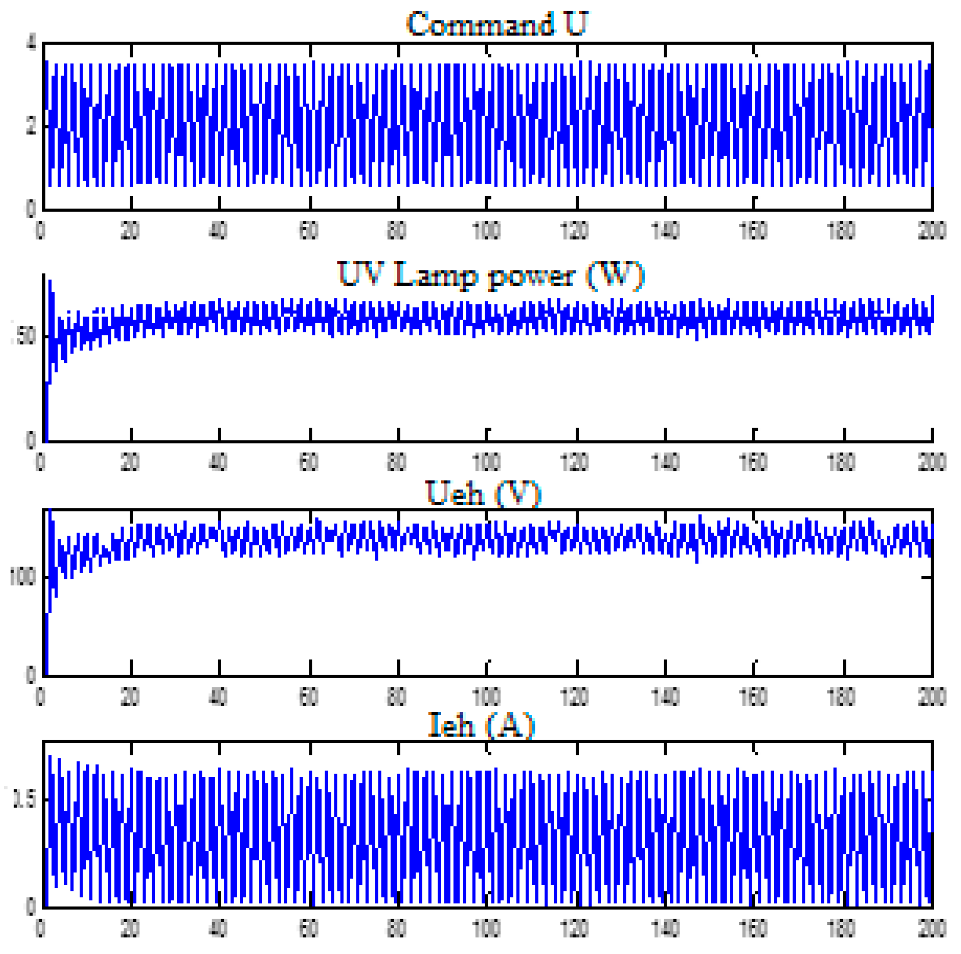
Figure 43.
Development of lighting, reference power for photovoltaic generators and reference voltage for GPV.
Figure 43.
Development of lighting, reference power for photovoltaic generators and reference voltage for GPV.
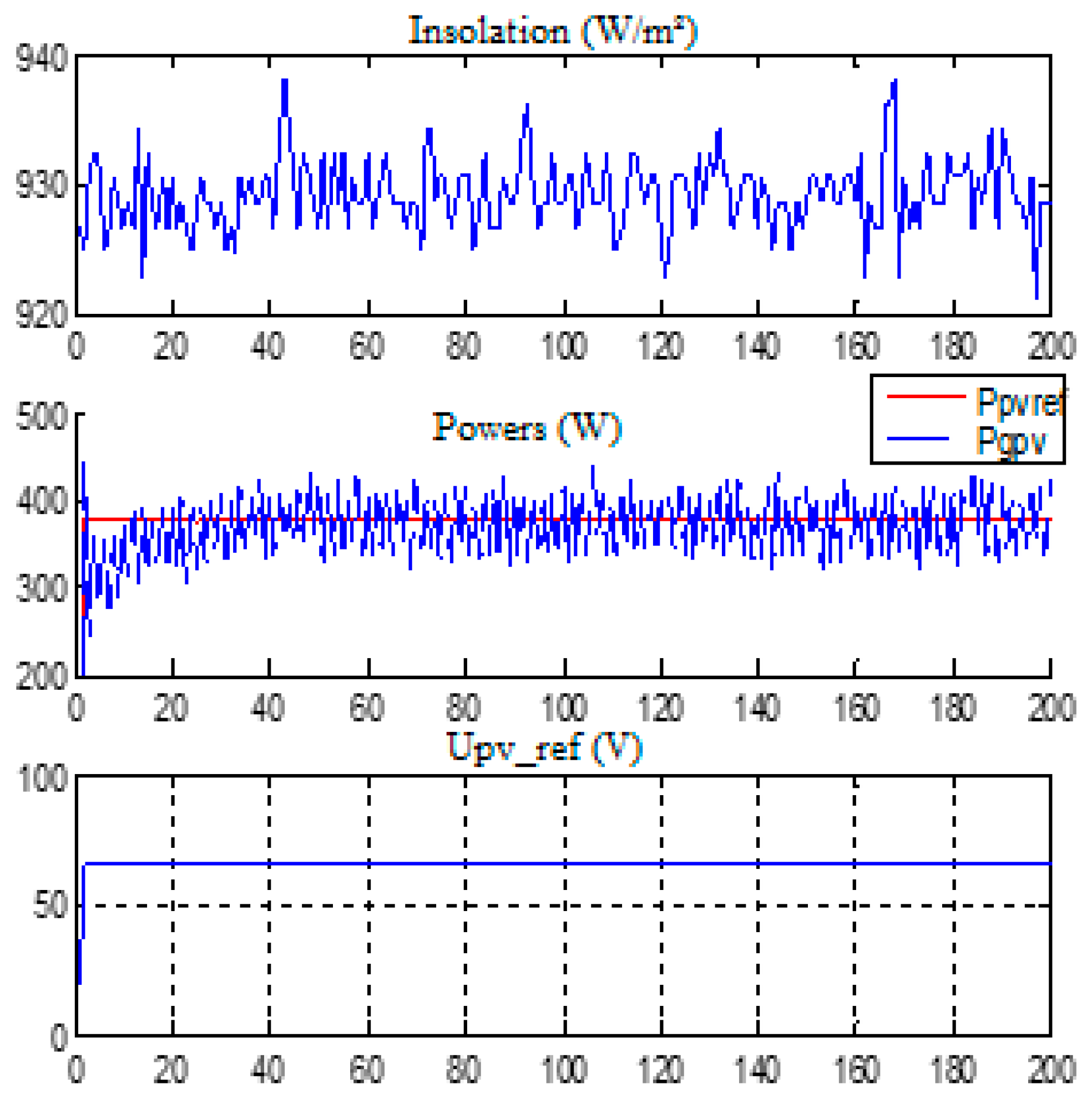
Figure 44.
Development of control law, power of UV lamp, input voltage of DC/DC converter () and input current of DC/DC converter ().
Figure 44.
Development of control law, power of UV lamp, input voltage of DC/DC converter () and input current of DC/DC converter ().

Figure 45.
Development of lighting, reference power for photovoltaic generators and reference voltage for GPV.
Figure 45.
Development of lighting, reference power for photovoltaic generators and reference voltage for GPV.
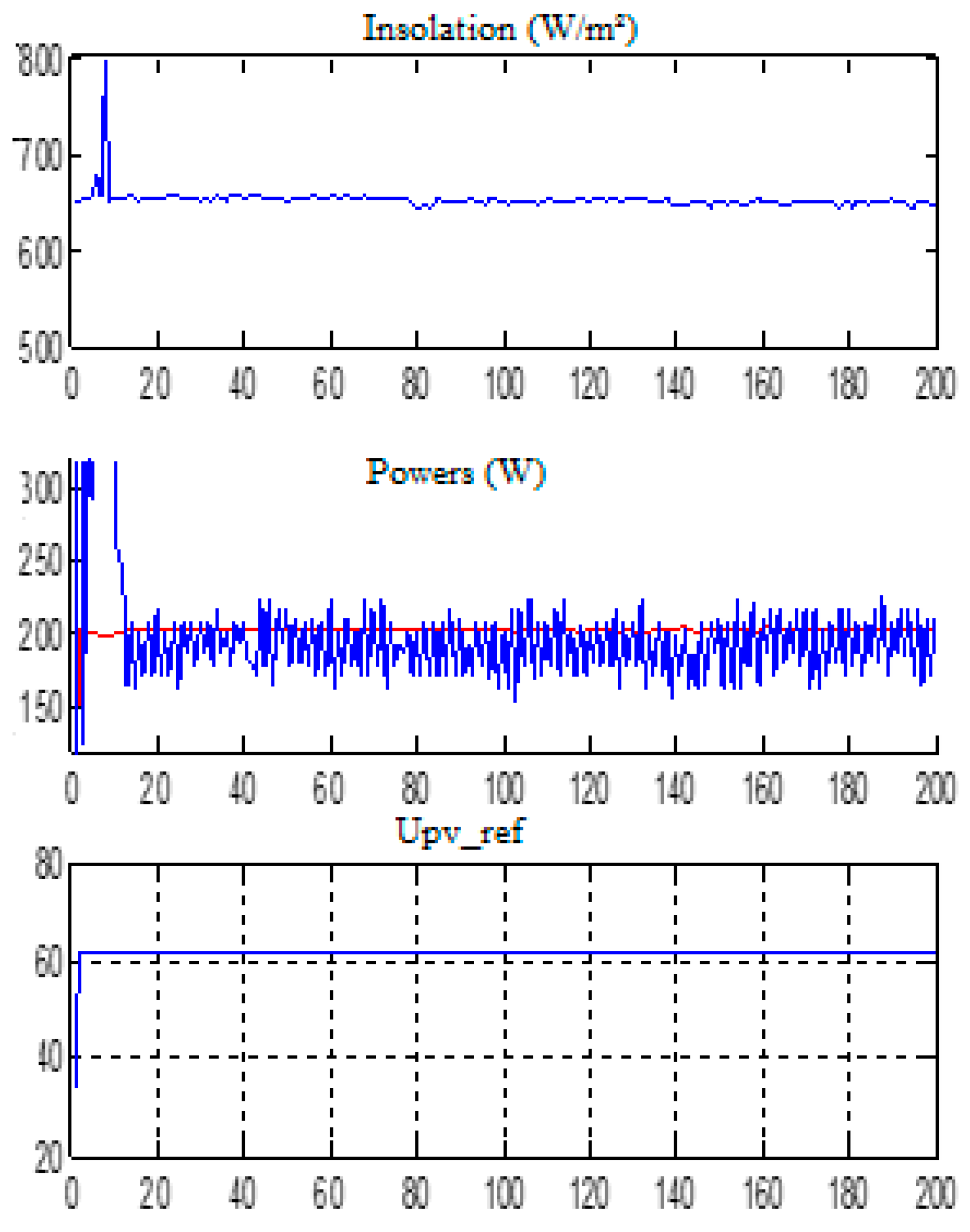
Figure 46.
Development of control law, power of UV lamp, input voltage of DC/DC converter () and input current of DC/DC converter ().
Figure 46.
Development of control law, power of UV lamp, input voltage of DC/DC converter () and input current of DC/DC converter ().

Figure 47.
Experimental and simulated curves of inactivation kinetics of Escherichia coli ATCC 29, [22].
Figure 47.
Experimental and simulated curves of inactivation kinetics of Escherichia coli ATCC 29, [22].

Table 1.
Effect of flow variation on the effectiveness of disinfection processes for water artificially contaminated by the strain of E. Parcel [22].
Table 1.
Effect of flow variation on the effectiveness of disinfection processes for water artificially contaminated by the strain of E. Parcel [22].
| D1 | D2 | D3 | D4 | D5 | |
|---|---|---|---|---|---|
| Debits (m3/h) | 0.023 | 0.039 | 0.081 | 0.15 | 0.25 |
| Depression U-Log10 | 4.3 | 3.7 | 2.39 | 1.67 | 1.18 |
| Efficiency (%) | 99.99 | 99.9 | 99.6 | 97.9 | 93.39 |
| Water quality | Adequate | Good | Not acceptable | Not acceptable | Not acceptable |
Table 2.
Extract from the prepared database [22].
Table 2.
Extract from the prepared database [22].
| UV Flux | Debits | Depression | Residence Time | Water Quality |
|---|---|---|---|---|
| 3.5 | 0.023 | 4.3 | 0.13 | Adequate |
| 3.65 | 0.031 | 4.28 | 0.096 | Adequate |
| 3.8 | 0.061 | 4.29 | 0.049 | Adequate |
| 4 | 0.072 | 4.31 | 0.041 | Adequate |
| 4.2 | 0.079 | 4.3 | 0.037 | Adequate |
| 4.35 | 0.086 | 4.28 | 0.033 | Adequate |
| 4.5 | 0.092 | 4.29 | 0.031 | Adequate |
| 4.65 | 0.101 | 4.27 | 0.029 | Adequate |
| 4.75 | 0.16 | 4.3 | 0.018 | Adequate |
| 5 | 0.21 | 4.29 | 0.014 | Adequate |
Disclaimer/Publisher’s Note: The statements, opinions and data contained in all publications are solely those of the individual author(s) and contributor(s) and not of MDPI and/or the editor(s). MDPI and/or the editor(s) disclaim responsibility for any injury to people or property resulting from any ideas, methods, instructions or products referred to in the content. |
© 2023 by the authors. Licensee MDPI, Basel, Switzerland. This article is an open access article distributed under the terms and conditions of the Creative Commons Attribution (CC BY) license (https://creativecommons.org/licenses/by/4.0/).
Share and Cite
MDPI and ACS Style
Zitouni, N.; Gammoudi, R.; Attafi, R.; Mezgahni, D. Developed and Intelligent Structure of a Control for PV Water Treatment System. Energies 2023, 16, 6540. https://doi.org/10.3390/en16186540
AMA Style
Zitouni N, Gammoudi R, Attafi R, Mezgahni D. Developed and Intelligent Structure of a Control for PV Water Treatment System. Energies. 2023; 16(18):6540. https://doi.org/10.3390/en16186540
Chicago/Turabian StyleZitouni, Naoufel, Rabiaa Gammoudi, Rim Attafi, and Dhafer Mezgahni. 2023. "Developed and Intelligent Structure of a Control for PV Water Treatment System" Energies 16, no. 18: 6540. https://doi.org/10.3390/en16186540
Note that from the first issue of 2016, this journal uses article numbers instead of page numbers. See further details here.