Battery and Hydrogen Energy Storage Control in a Smart Energy Network with Flexible Energy Demand Using Deep Reinforcement Learning

Abstract

Smart energy networks provide an effective means to accommodate high penetrations of variable renewable energy sources like solar and wind, which are key for the deep decarbonisation of energy production. However, given the variability of the renewables as well as the energy demand, it is imperative to develop effective control and energy storage schemes to manage the variable energy generation and achieve desired system economics and environmental goals. In this paper, we introduce a hybrid energy storage system composed of battery and hydrogen energy storage to handle the uncertainties related to electricity prices, renewable energy production, and consumption. We aim to improve renewable energy utilisation and minimise energy costs and carbon emissions while ensuring energy reliability and stability within the network. To achieve this, we propose a multi-agent deep deterministic policy gradient approach, which is a deep reinforcement learning-based control strategy to optimise the scheduling of the hybrid energy storage system and energy demand in real time. The proposed approach is model-free and does not require explicit knowledge and rigorous mathematical models of the smart energy network environment. Simulation results based on real-world data show that (i) integration and optimised operation of the hybrid energy storage system and energy demand reduce carbon emissions by 78.69%, improve cost savings by 23.5%, and improve renewable energy utilisation by over 13.2% compared to other baseline models; and (ii) the proposed algorithm outperforms the state-of-the-art self-learning algorithms like the deep-Q network.

1. Introduction

Globally, the energy system is responsible for about 73.2% of greenhouse gas emissions [1]. Deep reductions in greenhouse gas emissions in the energy system are key for achieving a net-zero greenhouse gas future to limit the rise in global temperatures to 1.5 °C and to prevent the daunting effects of climate change [2]. In response, the global energy system is undergoing an energy transition from the traditional high-carbon to a low- or zero-carbon energy system, mainly driven by enabling technologies like the internet of things [3] and the high penetration of variable renewable energy sources (RES) like solar and wind [4]. Although RESs are key for delivering a decarbonised energy system that is reliable, affordable, and fair for all, the uncertainties related to their energy generation as well as energy consumption remain a significant barrier, which is unlike the traditional high-carbon system with dispatchable sources [5].

Smart energy networks (SEN) (also known as micro-grids), which are autonomous local energy systems equipped with RESs and energy storage systems (ESS) as well as various types of loads, are an effective means of integrating and managing high penetrations of variable RESs in the energy system [6]. Given the uncertainties with RES energy generation as well as the energy demand, ESSs such as battery energy storage systems (BESS) have been proven to play a crucial role in managing the uncertainties while providing reliable energy services to the network [7]. However, due to low capacity density, BESSs cannot be used to manage high penetration of variable RESs [8].

Hydrogen energy storage systems (HESS) are emerging as promising high-capacity density energy storage carriers to support high penetrations of RESs. This is mainly due to falling costs for electricity from RESs and improved electrolyser technologies, whose costs have fallen by more than 60% since 2010 [9]. During periods of over-generation from the RESs, HESSs convert the excess power into hydrogen gas, which can be stored in a tank. The stored hydrogen can be sold externally as fuel such as for use in fuel-cell hybrid electric vehicles [10] or converted into power during periods of minimum generation from the RES to complement other ESSs such as the BESS.

The SEN combines power engineering with information technology to manage the generation, storage, and consumption to provide a number of technical and economic benefits, such as increased utilisation of RESs in the network, reduced energy losses and costs, increased power quality, and enhanced system stability [11]. However, this requires an effective smart control strategy to optimise the operation of the ESSs and energy demand to achieve the desired system economics and environmental outcomes.

Many studies have proposed control strategies that optimise the operation of ESSs to minimise utilisation costs [12,13,14,15]. Others have proposed control models for optimal sizing and planning of the microgrid [16,17,18]. Other studies have modeled the optimal energy sharing in the microgrid [19]. Despite a rich history, the proposed control approaches are model-based, in which they require explicit knowledge and rigorous mathematical models of the microgrid to capture complex real-world dynamics. Model errors and model complexity make it difficult to apply and optimise the ESSs in real-time. Moreover, even if an accurate and efficient model without errors exists, it is often a cumbersome and fallible process to develop and maintain the control approaches in situations where uncertainties of the microgrid are dynamic in nature [20].

In this paper, we propose a model-free control strategy based on reinforcement learning (RL), a machine learning paradigm, in which an agent learns the optimal control policy by interacting with the SEN environment [21]. Through trial and error, the agent selects control actions that maximise a cumulative reward (e.g., revenue) based on its observation of the environment. Unlike the model-based optimisation approaches, model-free-based algorithms do not require explicit knowledge and rigorous mathematical models of the environment, making them capable of determining optimal control actions in real-time even for complex control problems like peer-to-peer energy trading [22]. Further, artificial neural networks can be combined with RL to form deep reinforcement learning (DRL), making model-free approaches capable of handling even more complex control problems [23]. Examples of commonly used DRL-based algorithms are value-based algorithms such as Deep Q-networks (DQN) [23] and policy-based algorithms such as the deep deterministic policy gradient (DDPG) [24].

1.1. Related Works

The application of DRL approaches for managing SENs has increased in the past decade. However, much progress has been made for SENs having a single ESS (e.g., BESS) [11,20,25,26,27,28,29]. With declining costs of RESs, additional ESSs like HESS are expected in SENs to provide additional system flexibility and storage to support further deployment of RESs. In this case, control approaches that can effectively schedule the hybrid operation of BESSs and HESSs become imperative.

Recent studies on the optimised control of SENs having multiple ESSs like a hybrid of a BESS and a HESS are proposed in [8,30,31,32,33]. In [8,30], a DDPG-based algorithm is proposed to minimise building carbon emissions in an SEN that includes a BESS, an HESS, and constant building loads. Similarly, operating costs are minimised in [31] using DDPG and in [32] using DQN. However, these studies use a single control agent to manage the multiple ESSs. Energy management of an SEN is usually a multi-agent problem where an action of one agent affects the actions of others, making the SEN environment non-stationary from an agent’s perspective [22]. Single agents have been found to perform poorly in non-stationary environments [34].

A multi-agent-based control approach for the optimal operation of hydrogen-based multi-energy systems is proposed in [33]. Despite the approach addressing the drawbacks of the single agent, the flexibility of the electrical load is not investigated. With the introduction of flexible loads like heat pumps which run on electricity in SENs [35], the dynamics of the electrical load are expected to change the technical economics and the environmental impacts of the SEN.

Compared with the existing works, we investigate an SEN that has a BESS, an HESS, and a schedulable energy demand. We explore the energy cost and carbon emission minimisation problem of such an SEN while capturing the time-coupled storage dynamics of the BESS and the HESS, as well as the uncertainties related to RES, varying energy prices, and the flexible demand. A multi-agent deep deterministic policy gradient (MADDPG) algorithm is developed to reduce the system cost and carbon emissions and to improve the utilisation of RES while addressing the drawbacks of a single agent in a non-stationary environment. To the authors’ knowledge, this study is the first to comprehensively apply the MADDPG algorithm to optimally schedule the operation of the hybrid BESS and HESS as well as the energy demand in a SEN.

1.2. Contributions

The main contributions of this paper are on the following aspects:

• We formulate the SEN system cost minimisation problem, complete with a BESS, an HESS, flexible demand, and solar and wind generation, as well as dynamic energy pricing as a function of energy costs and carbon emissions cost. The system cost minimisation problem is then reformulated as a continuous action-based Markov game with unknown probability to adequately obtain the optimal energy control policies without explicitly estimating the underlying model of the SEN and relying on future information.
• A data-driven self-learning-based MADDPG algorithm that outperforms a model-based solution and other DRL-based algorithms used as a benchmark is proposed to solve the Markov game in real-time. This also includes the use of a novel real-world generation and consumption data set collected from the Smart Energy Network Demonstrator (SEND) project at Keele University [36].
• We conduct a simulation analysis of a SEN model for five different scenarios to demonstrate the benefits of integrating a hybrid of BESS and HESS and scheduling the energy demand in the network.
• Simulation results based on SEND data show that the proposed algorithm can increase cost savings and reduce carbon emissions by 41.33% and 56.3%, respectively, compared with other bench-marking algorithms and baseline models.

The rest of the paper is organised as follows. A description of the SEN environment is presented in Section 2. Formulation of the optimisation problem is given in Section 3. A brief background to RL and the description of the proposed self-learning algorithm is presented in Section 4. Simulation results are provided in Section 5, with conclusions presented in Section 6.

2. Smart Energy Network

The SEN considered in this paper is a grid-connected microgrid with a RES (solar and wind turbines), a hybrid energy storage system (BESS and HESS), and the electrical energy demand as shown in Figure 1. The aggregated electrical demand from the building(s) is considered to be a price-responsive demand i.e., the demand can be reduced based on electricity price variations or shifted from the expensive price time slots to the cheap price time slots. At every time slot t, solar and wind turbines provide energy to meet the energy demand. Any excess generation is either used to charge the BESS and/or converted into hydrogen by the electrolyser or exported to the main grid at a feed-in tariff ${\pi }_t$. In the event that energy generated from solar and wind turbines is insufficient to meet the energy demand, the deficit energy is either supplied by the BESS and/or fuel cell or imported from the main grid at a time-of-use (ToU) tariff ${\lambda }_t$.

In the following subsections, we present models of solar, wind, BESS, HESS (i.e., electrolyser, tank, and fuel cell), and flexible demand adopted in this paper.

2.1. PV and Wind Turbine Model

Instead of using mathematical equations to model the solar and wind turbine, we use real energy production data from the solar and the wind turbine, as these are undispatchable under normal SEN operating conditions. Thus, at every time step t, power generated from solar and wind turbines is modeled as $P_{pv,t}$ and $P_{w,t}$, respectively.

2.2. BESS Model

The key property of a BESS is the amount of energy it can store at time t. Let $P_{c,t}$ and $P_{d,t}$ be the charging and discharging power of the BESS, respectively. The BESS energy dynamics during charging and discharging operations can be modeled as follows [37]:

$$E_{t+1}^b=E_t^b+\left({\eta }_{c,t}{P}_{c,t}-\frac{P_{d,t}}{{\eta }_{d,t}}\right)\mathsf{\Delta }t,\forall t$$

(1)

where ${\eta }_{c,t}\in (0,1]$ and ${\eta }_{d,t}\in (0,1]$ are dynamic BESS charge and discharge efficiency as calculated in [38], respectively; $E_t^b$ is the BESS energy (kWh), and $\mathsf{\Delta }t$ is the duration of BESS charge or discharge.

The BESS charge level is limited by the storage capacity of the BESS as

$$E_{min}\le E_t^b\le E_{max}$$

(2)

where $E_{min}$ and $E_{max}$ are lower and upper boundaries of the BESS charge level.

To avoid charging and discharging the BESS at the same time, we have

$$P_{c,t}·P_{d,t}=0,\forall t$$

(3)

That is, at any particular time t, either $P_{c,t}$ or $P_{d,t}$ is zero. Further, the charging and discharging power is limited by maximum battery terminal power $P_{max}$ as specified by manufacturers as

$$0\le P_{c,t},P_{d,t}\le P_{max},\forall t$$

(4)

During operation, the BESS wear cannot be avoided due to repeated BESS charge and discharge processes. The wear cost can have a great impact on the economics of the SEN. The empirical wear cost of the BESS can be expressed as [39]

$$C_{BESS}^t=\frac{C_b^{ca}\left|E_t^b\right|}{L_c\times 2\times \mathrm{DoD}\times E_{nom}\times {({\eta }_{c,t}\times {\eta }_{d,t})}^2}$$

(5)

where $E_{nom}$ is the BESS nominal capacity, $C_b^{ca}$ is the BESS capital cost, DoD is the depth of discharge at which the BESS is cycled, and $L_c$ is the BESS life cycle.

2.3. HESS Model

In addition to the BESS, a HESS is considered in this study as a long-term energy storage unit. The HESS mainly consists of an electrolyser (EL), hydrogen storage tank (HT), and fuel cell (FC), as shown in Figure 1. The electrolyser uses the excess electrical energy from the RESs to produce hydrogen. The produced hydrogen gas is stored in the hydrogen storage tank and later used by the fuel cell to produce electricity whenever there is a deficit in energy generation in the SEN.

The dynamics of hydrogen in the tank associated with the generation and consumption of hydrogen by the electrolyser and fuel cell, respectively, is modeled as follows [12]:

$$H_{t+1}=H_t+\left(r_{el,t}{P}_{el,t}-\frac{P_{fc,t}}{r_{fc,t}}\right)\mathsf{\Delta }t,\forall t$$

(6)

where $P_{el,t}$ and $P_{fc,t}$ are the electrolyser power input and fuel cell output power, respectively; $H_t$ (in Nm${}^3$) is the hydrogen gas level in the tank; $r_{el,t}$ (in Nm${}^3$/kWh) and $r_{fc,t}$ (in kWh/Nm${}^3$) are the hydrogen generation and consumption ratios associated with the electrolyser and fuel cell, respectively.

The hydrogen level is limited by the storage capacity of the tank as

$$H_{min}\le H_t\le H_{max},\forall t$$

(7)

where $H_{min}$ and $H_{max}$ are the lower and upper boundaries imposed on the hydrogen level in the tank.

As the electrolyser and the fuel cell cannot operate at the same time, we have

$$P_{el,t}·P_{fc,t}=0,\forall t$$

(8)

Furthermore, power consumption and power generation, respectively associated with the electrolyser and fuel cell, are restricted to their rated values as

$$\begin{array}{cc}\hfill 0\le P_{el,t}& \le P_{max}^{el},\forall t\hfill \end{array}$$

(9)

$$\begin{array}{cc}\hfill 0\le P_{fc,t}& \le P_{max}^{fc},\forall t\hfill \end{array}$$

(10)

where $P_{max}^{el}$ and $P_{max}^{fc}$ are the rated power values of the electrolyser and fuel cell, respectively.

If the HESS is selected to store the excess energy, the cost of producing hydrogen through the electrolyser and later becoming fuel cell energy is given as [40]

$$C_t^{el-fc}=\frac{(C_{el}^{ca}/L_{el}+C_{el}^{om})+(C_{fc}^{ca}/L_{fc}+C_{fc}^{om})}{{\eta }_{fc,t}{\eta }_{el,t}}$$

(11)

where $C_{el}^{ca}$ and $C_{fc}^{ca}$ are electrolyser and fuel cell capital costs, $C_{el}^{om}$ and $C_{fc}^{om}$ are the operation and maintenance costs of the electrolyser and the fuel cell, ${\eta }_{el,t}$ and ${\eta }_{fc,t}$ are the electrolyser and fuel cell efficiencies, $L_{el}$ and $L_{fc}$ are the electrolyser and the fuel cell lifetimes, respectively.

The cost of meeting the deficit energy using the fuel cell with the hydrogen stored in the tank as fuel is given as [13]

$$\begin{array}{cc}\hfill C_t^{fc}=& \frac{C_{fc}^{ca}}{L_{fc}}+C_{fc}^{om}\hfill \end{array}$$

(12)

The total cost of operating the HESS at time t can be expressed as follows:

$$\begin{array}{c}\hfill C_{HESS}^t=\left\{\begin{array}{c}{C}_t^{el-fc},\mathrm{if}{P}_{el,t}>0\hfill \\ C_t^{fc},\mathrm{if}{P}_{fc,t}>0\hfill \\ 0,\mathrm{otherwise}\hfill \end{array}\right.\end{array}$$

(13)

2.4. Load Model

We assume that the total energy demand of the SEN has a certain proportion of flexible energy demand that can be reduced or shifted in time due to the energy price. Thus, at every time t, the actual demand may deviate from the expected total energy demand. Let the total energy demand before energy reduction be $D_t$ and the actual energy demand after reduction be $d_t$. Then, the energy reduction $\mathsf{\Delta }{d}_t$ can be expressed as

$$\begin{array}{c}\hfill \mathsf{\Delta }{d}_t=D_t-d_t\forall t\end{array}$$

(14)

As reducing the energy demand inconveniences the energy users, the $\mathsf{\Delta }{d}_t$ can be constrained as follows:

$$\begin{array}{c}\hfill 0\le \mathsf{\Delta }{d}_t\le \zeta D_t\forall tl\end{array}$$

(15)

where $\zeta$ (e.g., $\zeta =30\%$) is a constant factor that specifies the maximum percentage of original demand that can be reduced.

The inconvenience cost for reducing the energy demand can be estimated using a convex function as follows:

$$\begin{array}{c}\hfill C_{inc.}^t={\alpha }_d{\left(d_t-D_t\right)}^2\forall t\end{array}$$

(16)

where ${\alpha }_d$ is a small positive number that quantifies the amount of flexibility to reduce the energy demand, as shown in Figure 2. A lower value of ${\alpha }_d$ indicates that less attention is paid to the inconvenience cost and a larger share of the energy demand can be reduced to minimise the energy costs. A higher value of ${\alpha }_d$ indicates that high attention is paid to the inconvenience cost, and the energy demand can be hardly reduced to minimise the energy costs.

2.5. SEN Energy Balance Model

Local RES generation and demand in the SEN must be matched at all times for the stability of the energy system. Any energy deficit and excess must be imported and exported to the main grid, respectively.

The power import and export at time t can be expressed as

$$\begin{array}{c}\hfill P_{g,t}=d_t+P_{c,t}+P_{el,t}-P_{pv,t}-P_{w,t}-P_{d,t}-P_{fc,t}\end{array}$$

(17)

where $P_{g,t}$ is power import if $P_{g,t}>0$, and power export otherwise. We assume that the SEN is well-sized and that $P_{g,t}$ is always within the allowed export and import power limits.

Let ${\pi }_t$ and ${\lambda }_t$ be the export and import grid prices at time t, respectively. As grid electricity is the major source of carbon emissions, the cost of utilising the main grid to meet the supply–demand balance in the SEN is the sum of both the energy cost and the environmental cost due to carbon emissions as follows:

$$\begin{array}{c}\hfill C_{grid}^t=\mathsf{\Delta }t\left\{\begin{array}{c}{\lambda }_t{P}_{g,t}+{\mu }_c{P}_{g,t},\mathrm{if}{P}_{g,t}\ge 0\hfill \\ -{\pi }_t\left|P_{g,t}\right|,\mathrm{otherwise}\hfill \end{array}\right.\end{array}$$

(18)

where ${\mu }_c\in [0,1]$ is the carbon emission conversion factor of grid electricity.

3. Problem Formulation

The key challenge in operating the SEN is how to optimally schedule the operation of the BESS, the HESS, and the flexible energy demand to minimise energy costs and carbon emissions as well as to increase renewable energy utilisation. The operating costs associated with PV and wind generation are neglected for being comparatively smaller than those for energy storage units and energy demand [12].

3.1. Problem Formulation

As the only controllable assets in the SEN considered in this paper are the BESS, the HESS, and the flexible energy demand, the control variables can be denoted as a vector ${\mathbf{v}}_t=\{P_{c,t},P_{d,t},P_{el,t},P_{fc,t},\mathsf{\Delta }{d}_t\}$. $P_{g,t}$ can be obtained according to (17). We formulate an overall system cost-minimising problem as a function of the energy cost and the environmental cost as follows:

$$\mathbf{P}\mathbf{1}:\begin{array}{cc}\hfill \underset{{\mathbf{v}}_t}{min}:& \sum _{t=1}^T\left(C_{BESS}^t+C_{HESS}^t+C_{inc.}^t+C_{grid}^t\right)\hfill \\ \hfill \mathrm{s}.\mathrm{t}.:& \left(1\right)-\left(4\right)\&\left(6\right)-\left(10\right)\&\left(14\right),\left(15\right),\left(17\right)\hfill \end{array}$$

Solving this optimisation problem using model-based optimisation approaches suffers from three main challenges, namely uncertainties of parameters, information, and dimension challenges. The uncertainties are related to the RES, energy price, and energy demand, which makes it difficult to directly solve the optimisation problem without statistical information on the system. As expressed in (1) and (6), control of the BESS and HESS is time-coupled, and actions taken at time t have an effect on future actions to be taken at time $t+1$. Thus, for optimal scheduling, the control policies should also consider the future ‘unknown’ information of the BESS and the HESS. Moreover, the control actions of the BESS and the HESS are continuous in nature and bounded, as given in (4), (9), (10), which increases the dimension of the control problem.

In the following subsections, we overcome these challenges by first reformulating the optimisation problem as a continuous action Markov game and later solving it using a self-learning algorithm.

3.2. Markov Game Formulation

We reformulate P1 as a Markov decision process (MDP), which consists of a state space $\mathcal{S}$, an action space $\mathcal{A}$, a reward function $\mathcal{R}$, a discount factor $\gamma$, and a transition probability function $\mathcal{P}$, as follows:

3.2.1. State Space

The state space $\mathcal{S}$ represents the collection of all the state variables of the SEN at every time slot t, including RES variables ($P_{pv,t}\&P_{w,t}$), energy prices (${\pi }_t\&{\lambda }_t$), energy demand $D_t$, and state of the ESSs ($E_t^b\&H_t$). Thus, at time slot t, the state of the system is given as

$$s_t=\left(P_{pv,t},P_{w,t},E_{b,t},H_t,D_{n,t},{\pi }_t,{\lambda }_t\right),s_t\in \mathcal{S}$$

(19)

3.2.2. Action Space

The action space denotes the collection of all actions $\{P_{c,t},P_{d,t},P_{el,t},P_{fc,t},\mathsf{\Delta }{d}_t\}$, which are the decision values of P1 taken by the agents to produce the next state $s_{t+1}$ according to the state transition function $\mathcal{P}$. To reduce the size of the action space, action variables for each storage system can be combined into one action. With reference to (3), the BESS action variables $\{P_{c,t},P_{d,t}\}$ can be combined into one action $P_{b,t}$ so that during charging (i.e., $P_{b,t}<0$), $P_{c,t}=\left|P_{b,t}\right|\&P_{d,t}=0$. Otherwise, $P_{d,t}=P_{b,t}\&P_{c,t}=0$. Similarly, the HESS action variables $\{P_{el,t},P_{fc,t}\}$ can be combined into one action $P_{h,t}$. During electrolysis, (i.e., $P_{h,t}<0$), $P_{el,t}=\left|P_{h,t}\right|\&P_{fc,t}=0$. Otherwise, $P_{fc,t}=P_{h,t}\&P_{el,t}=0$. Thus, at time t, the control actions of the SEN reduce to

$$a_t=\left(P_{b,t},P_{h,t},\mathsf{\Delta }{d}_t\right),a_t\in \mathcal{A}$$

(20)

The action values are bounded according to their respective boundaries given by (4), (9), (10), and (15).

3.2.3. Reward Space

The collection of all the rewards received by the agents after interacting with the environment forms the reward space $\mathcal{R}$. The reward is used to evaluate the performance of the agent based on the actions taken and the state of the SEN observed by the agents at that particular time. The first part of the reward is the total energy cost and environmental cost of the SEN:

$$r_t^{\left(1\right)}=-\left(C_{BESS}^t+C_{HESS}^t+C_{inc.}^t+C_{grid}^t\right)$$

(21)

As constraints given in (2) and (7) should always be satisfied, the second part of the reward is a penalty for violating the constraints as follows:

$$\begin{array}{c}\hfill r_t^{\left(2\right)}=-\left\{\begin{array}{c}\mathcal{K},\mathrm{if}\left(2\right)\mathrm{or}\left(7\right)\mathrm{is}\mathrm{violated}\hfill \\ 0,\mathrm{otherwise}\hfill \end{array}\right.\end{array}$$

(22)

where $\mathcal{K}$ is a predetermined large number, e.g., $K=20$.

The total reward received by the agent after interacting with the environment is therefore expressed as

$$r_t=r_t^{\left(1\right)}+r_t^{\left(2\right)},r_t\in \mathcal{R}$$

(23)

The goal of the agent is to maximise its own expected reward R:

$$R=\sum _{t=0}^T{\gamma }^t{r}_t$$

(24)

where T is the time horizon and $\gamma$ is a discount factor, which helps the agent to focus the policy by caring more about obtaining the rewards quickly.

As electricity prices, RES energy generation, and demand are volatile in nature, it is generally impossible to obtain with certainty the state transition probability function $\mathcal{P}$ required to derive an optimal policy $\pi \left(s_t\right|a_t)$ needed to maximise R. To circumvent this difficulty, we propose the use of RL as discussed in Section 4.

4. Reinforcement Learning

4.1. Background

An RL framework is made up of two main components, namely the environment and the agent. The environment denotes the problem to be solved. The agent denotes the learning algorithm. The agent and environment continuously interact with each other [21].

At every time t, the agent learns for itself the optimal control policy $\pi \left(s_t\right|a_t)$ through trial and error by selecting control actions $a_t$ based on its perceived state $s_t$ of the environment. In return, the agent receives a reward $r_t$ and the next state $s_{t+1}$ from the environment without explicitly having knowledge of the transition probability function $\mathcal{P}$. The goal of the agent is to improve the policy so as to maximise the cumulative reward R. The environment has been described in Section 3. Next, we describe the learning algorithms.

4.2. Learning Algorithms

In this section, we present three main learning algorithms considered in this paper, namely DQN (a single-agent and value-based algorithm), DPPG (a single-agent and policy-based algorithm), and the proposed multi-agent DDPG (a multi-agent and policy-based algorithm).

4.2.1. DQN

The DQN algorithm was developed by Google DeepMind in 2015 [23]. It was developed to enhance a classic RL algorithm called Q-Learning [21] through the addition of deep neural networks and a novel technique called experience replay. In Q-learning, the agent learns the best policy $\pi \left(s_t\right|a_t)$ based on the notion of an action-value Q-function as $Q_{\pi }(s,a)={\mathbb{E}}_{\pi }\left[R|s_t=s,a_t=a\right]$. By exploring the environment, the agent updates the $Q_{\pi }(s,a)$ estimates using the Bellman equation as an iterative update as follows:

$$Q_{i+1}(s_t,a_t)\leftarrow Q_i(s_t,a_t)+\alpha h$$

(25)

where $\alpha \in (0,1]$ is the learning rate and h is given by

$$h=\left[r_t+\gamma \underset{a}{\max }{Q}_{\pi }(s_{t+1},a)-Q_i(s_t,a_t)\right]$$

(26)

Optimal Q-function $Q^{*}$ and policy ${\pi }^{*}$ are obtained when $Q_i(s_t,a_t)\to Q^{*}(s_t,a_t)$ as $i\to \infty$. As Q-learning represents the Q-function as a table containing values of all combinations of states and actions, it is impractical for most problems. The DQN algorithm addresses this by using a deep neural network with parameters $\theta$ to estimate the optimal Q-values, i.e., $Q(s_t,a_t;\theta )\approx Q^{*}(s_t,a_t)$ by minimising the following loss function $L\left(\theta \right)$ at each iteration i:

$$L_i\left({\theta }_i\right)=\mathbb{E}\left[{\left(y_i-Q(s_t,a_t;{\theta }_i)\right)}^2\right]$$

(27)

where $y_t=r_t+\gamma \underset{a}{\max }Q(s_{t+1},a_t;{\theta }_{i-1})$ is the target for iteration i.

To improve training and for better data efficiency, at each time step t, an experience, $e_t=\langle s_t,a_t,r_t,s_{t+1}\rangle$, is stored in a replay buffer $\mathcal{D}$. During training, the loss and its gradient are then computed using a minibatch of transitions sampled from the replay buffer. However, DQN and Q-learning both suffer from an overestimation problem as they both use the same action value to select and evaluate the Q-value function, making them impractical for problems with continuous action spaces.

4.2.2. DDPG

The DDPG algorithm is proposed to [24] to handle control problems with continuous action spaces, which otherwise are impractical to be handled by Q-learning and DQN. The DDPG consists of two independent neural networks: an actor and a critic network. The actor network is used to approximate the policy $\pi \left(s_t\right|a_t)$. The input to the actor network is the environment state $s_t$ and the output is the action $a_t$. The critic network is used to approximate the Q-function $Q(s_t,a_t)$ and is only used to train the agent, and the network is discarded during the deployment of the agent. The input to the critic network is the concatenation of the state $s_t$ and the action $a_t$ from the actor network, and the output is the Q-function $Q(s_t,a_t)$.

Similar to the DQN, the DDPG stores an experience, $e_t=\langle s_t,a_t,r_t,s_{t+1}\rangle$, in a replay buffer $\mathcal{D}$ at each time step t to improve training and for better data efficiency. To add more stability to the training, two target neural networks, which are identical to the (original) actor network and (original) critic network are also created. Let the network parameters of the original actor network, original critic network, target actor network, and target critic network be denoted as ${\theta }^{\mu }$, ${\theta }^Q$, ${\theta }^{{\mu }^{{}^{\prime }}}$, and ${\theta }^{Q^{{}^{\prime }}}$, respectively. Before training starts, ${\theta }^{\mu }$ and ${\theta }^Q$ are randomly initialised, and the ${\theta }^{{\mu }^{{}^{\prime }}}$ and ${\theta }^{Q^{{}^{\prime }}}$ are initialised as ${\theta }^{{\mu }^{{}^{\prime }}}\leftarrow {\theta }^{\mu }$ and ${\theta }^{Q^{{}^{\prime }}}\leftarrow {\theta }^Q$.

To train the original actor and critic networks, a minibatch of B experiences $\langle s_t^j,a_t^j,r_t^j,s_{t+1}^j\rangle {|}_{j=1}^B$, are randomly sampled from $\mathcal{D}$, where $j\in B$ is the sample index. The original critic network parameters ${\theta }^Q$ are updated through gradient descent using the mean-square Bellman error function:

$$L\left({\theta }^Q\right)=\frac{1}{B}\sum _{j=1}^B{\left(y_j-Q\left(s_t^j,a_t^j;{\theta }^Q\right)\right)}^2$$

(28)

where $Q\left(s_t^j,a_t^j;{\theta }^Q\right)$ is the predicted output of the original critic network and $y_j$ is its target value expressed as

$$y_j=r_t^j+\gamma Q^{{}^{\prime }}\left(s_{t+1}^j,{\mu }^{{}^{\prime }}(s_{t+1}^j;{\theta }^{{\mu }^{{}^{\prime }}});{\theta }^{Q^{{}^{\prime }}}\right)$$

(29)

where ${\mu }^{{}^{\prime }}(s_{t+1}^j;{\theta }^{{\mu }^{{}^{\prime }}})$ is the output (action) from the target actor-network and $Q^{{}^{\prime }}\left(s_{t+1}^j,{\mu }^{{}^{\prime }}(s_{t+1}^j;{\theta }^{{\mu }^{{}^{\prime }}});{\theta }^{Q^{{}^{\prime }}}\right)$ is the output (Q-value) from the target critic network.

At the same time, parameters of the original actor network are updated by maximising the policy objective function $J\left({\theta }^{\mu }\right)$:

$${\nabla }_{{\theta }^{\mu }}J\left({\theta }^{\mu }\right)=\frac{1}{B}\sum _{j=1}^B{\nabla }_{{\theta }^{\mu }}\mu \left(s;{\theta }^{\mu }\right){\nabla }_{a}Q\left(s,a;{\theta }^Q\right)$$

(30)

where $s=s_t^j$, $a=\mu (s_t^j;{\theta }^{\mu })$ is the output (action) from the original actor network and $Q\left(s,a;{\theta }^Q\right)$ is the output (Q-value) from the original critic network.

After the parameters of the original actor network and original critic network are updated, the parameters of the two target networks are updated through the soft update technique as

$$\left\{\begin{array}{c}{\theta }^{Q^{{}^{\prime }}}\leftarrow \tau {\theta }^Q+\left(1-\tau \right){\theta }^{Q^{{}^{\prime }}}\hfill \\ {\theta }^{{\mu }^{{}^{\prime }}}\leftarrow \tau {\theta }^{\mu }+\left(1-\tau \right){\theta }^{{\mu }^{{}^{\prime }}}\hfill \end{array}\right.$$

(31)

where $\tau$ is the learning rate.

To ensure that the agent explores the environment, a random process [41] is used to generate a noise ${\mathcal{N}}_t$, which is added to every action as follows:

$$a_t=\mu \left(s_t;{\theta }^{\mu }\right)+{\mathcal{N}}_t$$

(32)

However, as discussed in [34], the DDPG algorithm performs poorly in non-stationary environments.

4.3. The Proposed MADDPG Algorithm

Each controllable asset of the SEN (i.e., BESS, HESS, and flexible demand) can be considered an agent, making the SEN environment a multi-agent environment, as shown in Figure 3. With reference to Section 3, the state and action spaces for each agent can be defined as follows. The BESS agent’s state and action as $s_t^1=(P_{pv,t},P_{w,t},E_{b,t},D_{n,t},{\pi }_t,{\lambda }_t)$ and $a_t^1=\left(P_{b,t}\right)$, respectively. The HESS agent’s state and action as $s_t^2=(P_{pv,t},P_{w,t},D_{n,t},H_t,{\pi }_t,{\lambda }_t)$ and $a_t^2=\left(P_{h,t}\right)$, respectively, and the flexible demand agent’s state and action as $s_t^3=(P_{pv,t},P_{w,t},D_{n,t},{\pi }_t,{\lambda }_t)$ and $a_t^3=\left(\mathsf{\Delta }{d}_t\right)$, respectively. All the agents coordinate to maximise the same cumulative reward function given by (24).

With the proposed MADDPG algorithm, each agent is modelled as a DDPG agent, where, however, states and actions are shared between the agents during training, as shown in Figure 4. During training, the actor-network uses only the local state to calculate the actions, while the critic network uses the states and actions of all agents in the system to evaluate the local action. As the actions of all agents are known by each agent’s critic network, the entire environment is stationary during training. During execution, critic networks are removed and only actor networks are used. This means that with MADDPG, training is centralised while execution is decentralised.

A detailed pseudocode of the proposed algorithm is given in Algorithm 1.

Algorithm 1 MADDPG-based Optimal Control of an SEN

1: Initialise shared replay buffer $\mathcal{D}$ 2: for each agent $k=1,\cdots ,3$ do 3:    Randomly initialise (original) actor and critic networks with parameters ${\theta }^{\mu }$ and ${\theta }^Q$, respectively 4:    Initialise (target) actor and critic networks as ${\theta }^{{\mu }^{{}^{\prime }}}\leftarrow {\theta }^{\mu }$ and ${\theta }^{Q^{{}^{\prime }}}\leftarrow {\theta }^Q$ respectively 5: end for 6: for each episode $eps=1,2,\cdots ,M$ do 7:    for each agent $k=1,\cdots ,3$ do 8:      Initialise a random process ${\mathcal{N}}_t$ for exploration 9:      Observe initial state $s_t^k$ from the environment 10:    end for 11:    for each time step $t=1,2,\cdots ,T$ do 12:      for each agent $k=1,\cdots ,3$ do 13:         Select an action according to (32) 14:      end for 15:      Execute joint action ${\mathbf{a}}_t=\langle a_t^1,a_t^2,a_t^3\rangle$ 16:      for each agent $k=1,\cdots ,3$ do 17:         Collect reward $r_t^k$ and observe state $s_{t+1}^k$ 18:         Store $〈a_t^k,s_t^k,r_t^k,s_{t+1}^k〉$ into $\mathcal{D}$ 19:         Update $s_t^k$←$s_{t+1}^k$ 20:         Randomly sample minibatch of B transitions $〈a_t^j,s_t^j,r_t^j,s_{t+1}^j〉{|}_{j=1}^B$ from $\mathcal{D}$ 21:         Update (original) critic network by (28) 22:         Update (original) actor network by (30) 23:         Update target networks by (31) 24:      end for 25:    end for 26: end for

5. Simulation Results

5.1. Experimental Setup

In this paper, real-world RES (solar and wind) generation and consumption data, which are obtained from the Smart Energy Network Demonstrator (SEND), are used for the simulation studies [36]. We use the UK’s time-of-use (ToU) electricity price as grid electricity buying price, which is divided into peak price 0.234 GBP/kWh (4 pm–8 pm), flat price 0.117 GBP/kWh (2 pm–4 pm and 8 pm–11 pm), and the valley price 0.07 GBP/kWh (11 pm–2 pm). The electricity price for selling electricity back to the main grid is a flat price ${\pi }_t=$ 0.05 GBP/kWh, which is lower than the ToU to avoid any arbitrage behaviour by the BESS and HESS. A carbon emission conversion factor ${\mu }_c=0.23314$ kg CO${}_2$/kWh, is used to quantify the carbon emissions generated for using electricity from the main grid to meet the energy demand in the SEN [42]. We set the initial BESS state of charge and hydrogen level in the tank as $E_0=1.6$ MWh and $H_0=5$ Nm${}^3$, respectively. Other technical–economic parameters of the BESS and HESS are tabulated in

Table 1. BESS and HESS simulation parameters.

ESS	Parameter and Value
BESS	$E_{nom}=$ 2 MWh, $P_{max}=102$ kW, $DoD=$ 80%
	$E_{min}=$ 0.1 MWh, $E_{max}=$ 1.9 MWh, $L_c=$ 3650
	$C_b^{ca}$ = £210,000, ${\eta }_{c,t}={\eta }_{d,t}=$ 98%
HESS	$H_{min}=$ 2 Nm${}^3$, $H_{max}=$ 10 Nm${}^3$, $P_{max}^{el}=$ 3 kW
	$P_{max}^{fc}=$ 3 kW, ${\eta }_{fc,t}=$ 50%, ${\eta }_{el,t}=$ 90%
	$L_{fc}=L_{el}=30,000$ h, $r_{fc,t}=$ 0.23 Nm${}^3$/kWh
	$r_{el,t}=$1.32 kWh/Nm${}^3$, $C_{el}^{om}=C_{fc}^{om}$= £0.174/h
	$C_{el}^{ca}$ = £60,000, $C_{fc}^{ca}$= £22,000

. A day is divided into 48 time slots, i.e., each time slot is equivalent to 30 min.

The actor and critic networks for each MADDPG agent are designed using hyperparameters tabulated in

Table 2. Hyperparameters for each actor and critic network.

Hyperparameter	Actor Network	Critic Network
Optimiser	Adam	Adam
Batch size	256	256
Discount factor	0.95	0.95
Learning rate	$1\times {10}^{-4}$	$3\times {10}^{-4}$
No. of hidden layers	2	2
No. of neurons	500	500

. We use the rectified linear unit (ReLU) as an activation function for the hidden layers and the output of the critic networks. A Tanh activation function is used in the output layer of each actor-network. We set the capacity of the replay buffer to be K = $1\times {10}^6$ and the maximum training steps in an episode to be $T=48$. Algorithm 1 is developed and implemented in Python using PyTorch framework [43].

5.2. Benchmarks

We verify the performance of the proposed MADDPG algorithm by comparing it with other three bench-marking algorithms:

• Rule-based (RB) algorithm: This is a model-based algorithm that follows the standard practice of wanting to meet the energy demand of the SEN using the RES generation without guiding the operation of the BESS, HESS, and flexible demands towards periods of low/high electricity price to save energy costs. In the event that there is surplus energy generation, the surplus is first stored in the short-term BESS, followed by the long-term HESS, and any extra is sold to the main grid. If the energy demand exceeds RES generation, the deficit is first provided by the BESS followed by the HESS, and then the main grid.
• DQN algorithm: As discussed in Section 4, this is a value-based DRL algorithm, which intends to optimally schedule the operation of the BESS, HESS, and flexible demand using a single agent and a discretised action space.
• DDPG algorithm: This is a policy-based DRL algorithm, which intends to optimally schedule the operation of the BESS, HESS, and flexible demand using a single agent and a continuous action space, as discussed in Section 4.

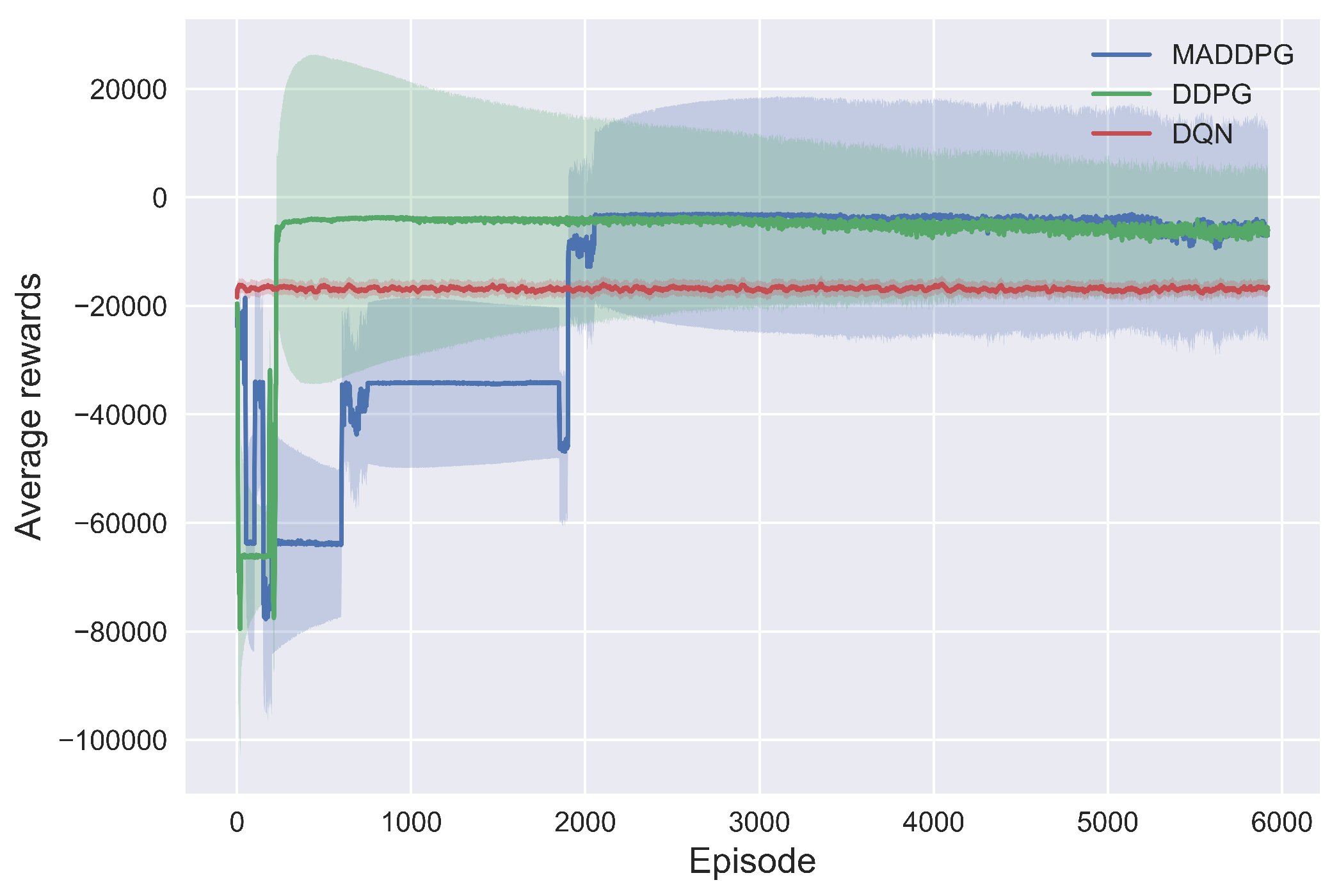
5.3. Algorithm Convergence

We analyse the convergence of the MADDPG algorithm by training the agents with 5900 episodes, with each episode having 48 training steps. In Figure 5, the average rewards obtained for each episode are plotted against the episodes and compared to the DRL-based bench-marking algorithms.

As shown in Figure 5, all algorithms achieve convergence after 2000 episodes. The DQN reaches convergence faster than MADDPG and DDPG due to the DQN’s discretised and low-dimensional action space, making the determination of the optimal scheduling policy relatively easier and quicker than the counterpart algorithms with continuous and high-dimensional action spaces. As a discretised action space cannot accurately capture the complexity and dynamics of the SEN energy management, the DQN algorithm converges to the worst optimal policy given by the lowest average reward value (−16,572.5). On the other hand, the MADDPG algorithm converges to a high average reward value (−6858.1), which is slightly higher than the reward value (−8361.8) for the DDPG, mainly due to enhanced cooperation between the operation of the controlled assets.

5.4. Algorithm Performance

In this section, we demonstrate the effectiveness of the proposed algorithm for optimally scheduling the BESS, the HESS, and the flexible demand to minimise the energy and environmental costs. Figure 6 shows the scheduling results in response to the SEN net demand for a period of 7 days, i.e., $T=336$ h. As shown in Figure 6, the BESS and HESS accurately charge (negative power) and discharge (positive power) whenever the net demand is negative (i.e., RES generation exceeds energy demand) and positive (i.e., energy demand exceeds RES generation), respectively. Similarly, the scheduled demand is observed to be high and low whenever the net demand is negative and positive, respectively.

Figure 7 shows that in order to minimise the multi-objective function given by $\mathbf{P}\mathbf{1}$, the algorithm prioritises the flexible demand agent to aggressively respond to price changes compared to the BESS and HESS agents. As shown in Figure 7, the scheduled demand reduces sharply whenever the electricity price is the highest, and increases when the price is lowest compared to the actions by the BESS and HESS.

Together, Figure 6 and Figure 7 demonstrate how the algorithm allocates different priorities to the agents to achieve a collective goal: minimise carbon costs, energy, and operational costs. In this case, the BESS and HESS agents are trained to respond more aggressively to changes in energy demand and generation, and maximise the benefits thereof like minimum carbon emissions. On the other hand, scheduling the flexible demand guides the SEN towards low energy costs.

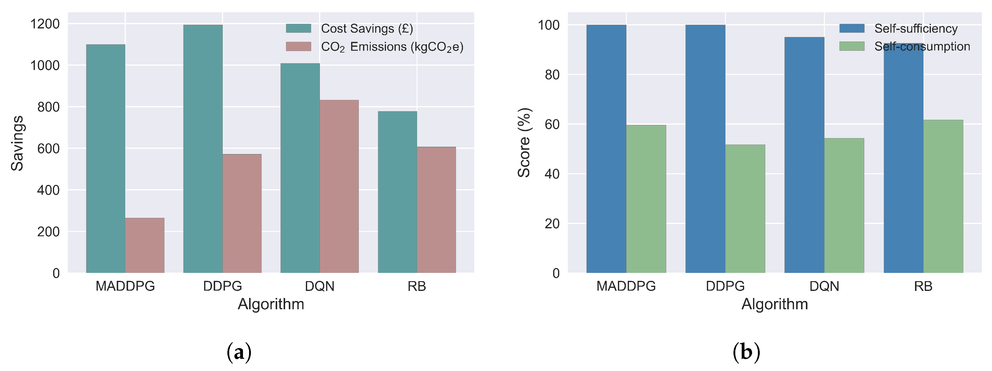
5.5. Improvement in Cost Saving and Carbon Emission

To demonstrate the economic and environmental benefits of integrating the BESS and the HESS in the SEN, the MADDPG algorithm was tested on different SEN models as shown in

Table 3. Cost savings and carbon emissions for different SEN models. A tick (✔) indicates that a model is considered and a cross (×) indicates that a model is not considered.

Models	Proposed	No BESS	No HESS	No Flex. Demand	No Assets
BESS	✔	×	✔	✔	×
HESS	✔	✔	×	✔	×
Flex. Demand	✔	✔	✔	×	×
Cost Saving (£)	1099.60	890.36	1054.58	554.01	451.26
Carbon Emission (kg CO${}_2$e)	265.25	1244.70	521.92	1817.37	2175.66

. The SEN models differ based on whether the SEN has any of the controllable assets; BESS, HESS, and flexible demand or not. For example, the SEN model that only has HESS and flexible demand as controllable assets is denoted as ‘No BESS’. The total cost savings and carbon emissions for each model were obtained as a sum of the cost savings and carbon emissions obtained half-hourly for 7 days.

As shown in Table 3, integrating BESS and HESS in the SEN as well as scheduling the energy demand achieves the highest cost savings and reduction in carbon emission. For example, the cost savings and carbon emissions are 23.5% and 78.69% higher and lower, respectively, than those for the SEN model without BESS (i.e., the ‘No BESS’ model), mainly due to improved RES utilisation for the proposed SEN model.

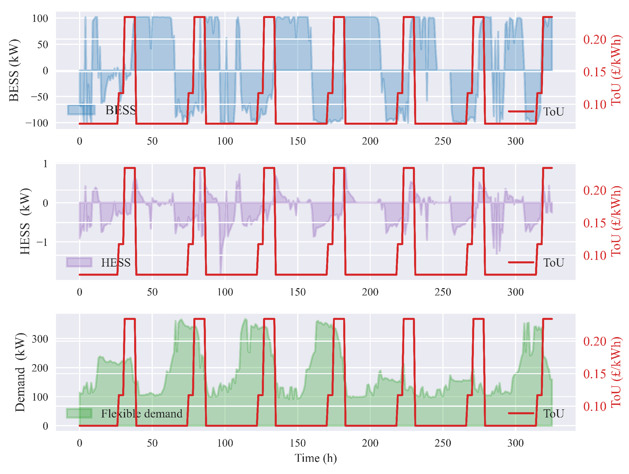
5.6. Improvement in RES Utilisation

To demonstrate improvement in RES utilisation as a result of integrating the BESS and the HESS in the SEN as well as scheduling energy demand, we use self-consumption and self-sufficiency as performance metrics. Self-consumption is defined as a ratio of RES generation used by the SEN (i.e., to meet the energy demand and to charge the BESS and HESS) to the overall RES generation [44]. Self-sufficiency is defined as the ratio of the energy demand that is supplied by the RES, BESS, and HESS to the overall energy demand [45].

Table 4. Self-consumption and self-sufficiency for different SEN models. A tick (✔) indicates that a model is considered and a cross (×) indicates that a model is not considered.

Models	Proposed	No BESS	No HESS	No Flex. Demand	No Assets
BESS	✔	×	✔	✔	×
HESS	✔	✔	×	✔	×
Flex. Demand	✔	✔	✔	×	×
Self-consumption	59.6%	48.0%	39.2%	46.0%	50.0%
Self-sufficiency	100%	85.3%	95.2%	78.8%	73.4%

shows that integrating the BESS and the HESS in the SEN as well as scheduling energy demand improves RES utilisation. Overall, the proposed SEN model achieved the highest RES utilisation, with 59.6% self-consumption and 100% self-sufficiency. This demonstrates the potential of integrating HESS in future SENs for absorbing more RES, thereby accelerating the rate of power system decarbonisation.

5.7. Algorithm Evaluation

The performance of the proposed MADDPG algorithm was evaluated by comparing it to the bench-marking algorithms for cost savings, carbon emissions, self-consumption, and self-sufficiency, as shown in Figure 8.

The MADDPG algorithm obtained the most stable and competitive performance in all the performance metrics considered, i.e., cost savings, carbon emissions, self-consumption, and self-sufficiency. This is mainly due to its multi-agent feature, which ensures a better learning experience in the environment. For example, the MADDPG improved the cost savings and reduced carbon emissions by 41.33% and 56.3%, respectively, relative to the RB approach. The rival DDPG algorithm achieved the highest cost savings at the expense of carbon emissions and self-sufficiency. As more controllable assets are expected in future SENs due to the digitisation of power systems, multi-agent-based algorithms are therefore expected to play a key energy management role.

5.8. Sensitivity Analysis of Parameter ${\alpha }_d$

The parameter ${\alpha }_d$ quantifies the amount of flexibility to reduce the energy demand. A lower value of ${\alpha }_d$ indicates that less attention is paid to the inconvenience cost, and a larger share of the energy demand can be reduced to minimise the energy costs. A higher value of ${\alpha }_d$ indicates that high attention is paid to the inconvenience cost and the energy demand can be hardly reduced to minimise the energy costs. With the change in ${\alpha }_d$ values, the cost savings and carbon emission results are compared in Figure 9.

As shown in Figure 9, the cost savings and carbon emissions reduce and increase, respectively, as ${\alpha }_d$ takes values from 0.0001 to 0.001, which means that the energy demand’s sensitivity to price reduces with increased inconvenience levels as given by (16). Thus, having an energy demand that is sensitive to electricity prices is crucial for reducing carbon emissions and promoting the use of RESs.

6. Conclusions

In this paper, we investigated the problem of minimising energy costs and carbon emissions as well as increasing renewable energy utilisation in a smart energy network (SEN) with BESS, HESS, and schedulable energy demand. A multi-agent deep deterministic policy gradient algorithm was proposed as a real-time control strategy to optimally schedule the operation of the BESS, HESS, and schedulable energy demand while ensuring that the operating constraints and time-coupled storage dynamics of the BESS and HESS are achieved. Simulation results based on real-world data showed increased cost savings, reduced carbon emissions, and improved renewable energy utilisation with the proposed algorithm and SEN. On average, the cost savings and carbon emissions were 23.5% and 78.69% higher and lower, respectively, with the proposed SEN model than baseline SEN models. The simulation results also verified the efficacy of the proposed algorithm to manage the SEN outperforming other bench-marking algorithms, including DDPG and DQN algorithms. Overall, the results have shown great potential for integrating HESS in SENs and using self-learning algorithms to manage the operation of the SEN.

References

1. Ritchie, H.; Roser, M.; Rosado, P. Carbon Dioxide and Greenhouse Gas Emissions, Our World in Data. 2020. Available online: https://ourworldindata.org/co2-and-greenhouse-gas-emissions (accessed on 10 July 2023).
2. Allen, M.R.; Babiker, M.; Chen, Y.; de Coninck, H.; Connors, S.; van Diemen, R.; Dube, O.P.; Ebi, K.L.; Engelbrecht, F.; Ferrat, M.; et al. Summary for policymakers. In Global Warming of 1.5: An IPCC Special Report on the Impacts of Global Warming of 1.5 °C above Pre-Industrial Levels and Related Global Greenhouse Gas Emission Pathways, in the Context of Strengthening the Global Response to the Threat of Climate Change, Sustainable Development, and Efforts to Eradicate Poverty; IPCC: Geneva, Switzerland, 2018. [Google Scholar]
3. Fuller, A.; Fan, Z.; Day, C.; Barlow, C. Digital twin: Enabling technologies, challenges and open research. IEEE Access 2020, 8, 108952–108971. [Google Scholar] [CrossRef]
4. Bouckaert, S.; Pales, A.F.; McGlade, C.; Remme, U.; Wanner, B.; Varro, L.; D’Ambrosio, D.; Spencer, T. Net Zero by 2050: A Roadmap for the Global Energy Sector; International Energy Agency: Paris, France, 2021.
5. Paul, D.; Ela, E.; Kirby, B.; Milligan, M. The Role of Energy Storage with Renewable Electricity Generation; National Renewable Energy Laboratory: Golden, CO, USA, 2010.
6. Harrold, D.J.; Cao, J.; Fan, Z. Renewable energy integration and microgrid energy trading using multi-agent deep reinforcement learning. Appl. Energy 2022, 318, 119151. [Google Scholar] [CrossRef]
7. Arbabzadeh, M.; Sioshansi, R.; Johnson, J.X.; Keoleian, G.A. The role of energy storage in deep decarbonization of electricity production. Nature Commun. 2019, 10, 3414. [Google Scholar] [CrossRef]
8. Desportes, L.; Fijalkow, I.; Andry, P. Deep reinforcement learning for hybrid energy storage systems: Balancing lead and hydrogen storage. Energies 2021, 14, 4706. [Google Scholar] [CrossRef]
9. Qazi, U.Y. Future of hydrogen as an alternative fuel for next-generation industrial applications; challenges and expected opportunities. Energies 2022, 15, 4741. [Google Scholar] [CrossRef]
10. Correa, G.; Muñoz, P.; Falaguerra, T.; Rodriguez, C. Performance comparison of conventional, hybrid, hydrogen and electric urban buses using well to wheel analysis. Energy 2017, 141, 537–549. [Google Scholar] [CrossRef]
11. Harrold, D.J.; Cao, J.; Fan, Z. Battery control in a smart energy network using double dueling deep q-networks. In Proceedings of the 2020 IEEE PES Innovative Smart Grid Technologies Europe (ISGT-Europe), Virtual, 26–28 October 2020; pp. 106–110. [Google Scholar]
12. Vivas, F.; Segura, F.; Andújar, J.; Caparrós, J. A suitable state-space model for renewable source-based microgrids with hydrogen as backup for the design of energy management systems. Energy Convers. Manag. 2020, 219, 113053. [Google Scholar] [CrossRef]
13. Cau, G.; Cocco, D.; Petrollese, M.; Kær, S.K.; Milan, C. Energy management strategy based on short-term generation scheduling for a renewable microgrid using a hydrogen storage system. Energy Convers. Manag. 2014, 87, 820–831. [Google Scholar] [CrossRef]
14. Enayati, M.; Derakhshan, G.; Hakimi, S.M. Optimal energy scheduling of storage-based residential energy hub considering smart participation of demand side. J. Energy Storage 2022, 49, 104062. [Google Scholar] [CrossRef]
15. HassanzadehFard, H.; Tooryan, F.; Collins, E.R.; Jin, S.; Ramezani, B. Design and optimum energy management of a hybrid renewable energy system based on efficient various hydrogen production. Int. J. Hydrogen Energy 2020, 45, 30113–30128. [Google Scholar] [CrossRef]
16. Castaneda, M.; Cano, A.; Jurado, F.; Sánchez, H.; Fernández, L.M. Sizing optimization, dynamic modeling and energy management strategies of a stand-alone pv/hydrogen/battery-based hybrid system. Int. J. Hydrogen Energy 2013, 38, 3830–3845. [Google Scholar] [CrossRef]
17. Liu, J.; Xu, Z.; Wu, J.; Liu, K.; Guan, X. Optimal planning of distributed hydrogen-based multi-energy systems. Appl. Energy 2021, 281, 116107. [Google Scholar] [CrossRef]
18. Pan, G.; Gu, W.; Lu, Y.; Qiu, H.; Lu, S.; Yao, S. Optimal planning for electricity-hydrogen integrated energy system considering power to hydrogen and heat and seasonal storage. IEEE Trans. Sustain. Energy 2020, 11, 2662–2676. [Google Scholar] [CrossRef]
19. Tao, Y.; Qiu, J.; Lai, S.; Zhao, J. Integrated electricity and hydrogen energy sharing in coupled energy systems. IEEE Trans. Smart Grid 2020, 12, 1149–1162. [Google Scholar] [CrossRef]
20. Nakabi, T.A.; Toivanen, P. Deep reinforcement learning for energy management in a microgrid with flexible demand. Sustain. Energy Grids Netw. 2021, 25, 100413. [Google Scholar] [CrossRef]
21. Sutton, R.S.; Barto, A.G. Reinforcement Learning: An Introduction; MIT Press: Cambridge, MA, USA, 2018. [Google Scholar]
22. Samende, C.; Cao, J.; Fan, Z. Multi-agent deep deterministic policy gradient algorithm for peer-to-peer energy trading considering distribution network constraints. Appl. Energy 2022, 317, 119123. [Google Scholar] [CrossRef]
23. Mnih, V.; Kavukcuoglu, K.; Silver, D.; Rusu, A.A.; Veness, J.; Bellemare, M.G.; Graves, A.; Riedmiller, M.; Fidjeland, A.K.; Ostrovski, G.; et al. Human-level control through deep reinforcement learning. Nature 2015, 518, 529–533. [Google Scholar] [CrossRef]
24. Lillicrap, T.P.; Hunt, J.J.; Pritzel, A.; Heess, N.; Erez, T.; Tassa, Y.; Silver, D.; Wierstra, D. Continuous control with deep reinforcement learning. arXiv Prep. 2015, arXiv:1509.02971. [Google Scholar]
25. Wan, T.; Tao, Y.; Qiu, J.; Lai, S. Data-driven hierarchical optimal allocation of battery energy storage system. IEEE Trans. Sustain. Energy 2021, 12, 2097–2109. [Google Scholar] [CrossRef]
26. Bui, V.-H.; Hussain, A.; Kim, H.-M. Double deep q -learning-based distributed operation of battery energy storage system considering uncertainties. IEEE Trans. Smart Grid 2020, 11, 457–469. [Google Scholar] [CrossRef]
27. Sang, J.; Sun, H.; Kou, L. Deep reinforcement learning microgrid optimization strategy considering priority flexible demand side. Sensors 2022, 22, 2256. [Google Scholar] [CrossRef]
28. Gao, S.; Xiang, C.; Yu, M.; Tan, K.T.; Lee, T.H. Online optimal power scheduling of a microgrid via imitation learning. IEEE Trans. Smart Grid 2022, 13, 861–876. [Google Scholar] [CrossRef]
29. Mbuwir, B.V.; Geysen, D.; Spiessens, F.; Deconinck, G. Reinforcement learning for control of flexibility providers in a residential microgrid. IET Smart Grid 2020, 3, 98–107. [Google Scholar] [CrossRef]
30. Chen, T.; Gao, C.; Song, Y. Optimal control strategy for solid oxide fuel cell-based hybrid energy system using deep reinforcement learning. IET Renew. Power Gener. 2022, 16, 912–921. [Google Scholar] [CrossRef]
31. Zhu, Z.; Weng, Z.; Zheng, H. Optimal operation of a microgrid with hydrogen storage based on deep reinforcement learning. Electronics 2022, 11, 196. [Google Scholar] [CrossRef]
32. Tomin, N.; Zhukov, A.; Domyshev, A. Deep reinforcement learning for energy microgrids management considering flexible energy sources. In EPJ Web of Conferences; EDP Sciences: Les Ulis, France, 2019; Volume 217, p. 01016. [Google Scholar]
33. Yu, L.; Qin, S.; Xu, Z.; Guan, X.; Shen, C.; Yue, D. Optimal operation of a hydrogen-based building multi-energy system based on deep reinforcement learning. arXiv 2021, arXiv:2109.10754. [Google Scholar]
34. Lowe, R.; Wu, Y.I.; Tamar, A.; Harb, J.; Abbeel, O.P.; Mordatch, I. Multi-agent actor-critic for mixed cooperative-competitive environments. Adv. Neural Inf. Process. Syst. 2017, 30. [Google Scholar] [CrossRef]
35. Wright, G. Delivering Net Zero: A Roadmap for the Role of Heat Pumps, HPA. Available online: https://www.heatpumps.org.uk/wp-content/uploads/2019/11/A-Roadmap-for-the-Role-of-Heat-Pumps.pdf (accessed on 26 May 2023).
36. Keele University, The Smart Energy Network Demonstrator. Available online: https://www.keele.ac.uk/business/businesssupport/smartenergy/ (accessed on 19 September 2023).
37. Samende, C.; Bhagavathy, S.M.; McCulloch, M. Distributed state of charge-based droop control algorithm for reducing power losses in multi-port converter-enabled solar dc nano-grids. IEEE Trans. Smart Grid 2021, 12, 4584–4594. [Google Scholar] [CrossRef]
38. Samende, C.; Bhagavathy, S.M.; McCulloch, M. Power loss minimisation of off-grid solar dc nano-grids—Part ii: A quasi-consensus-based distributed control algorithm. IEEE Trans. Smart Grid 2022, 13, 38–46. [Google Scholar] [CrossRef]
39. Han, S.; Han, S.; Aki, H. A practical battery wear model for electric vehicle charging applications. Appl. Energy 2014, 113, 1100–1108. [Google Scholar] [CrossRef]
40. Dufo-Lopez, R.; Bernal-Agustín, J.L.; Contreras, J. Optimization of control strategies for stand-alone renewable energy systems with hydrogen storage. Renew. Energy 2007, 32, 1102–1126. [Google Scholar] [CrossRef]
41. Uhlenbeck, G.E.; Ornstein, L.S. On the theory of the brownian motion. Phys. Rev. 1930, 36, 823. [Google Scholar] [CrossRef]
42. RenSMART, UK CO2(eq) Emissions due to Electricity Generation. Available online: https://www.rensmart.com/Calculators/KWH-to-CO2 (accessed on 20 June 2023).
43. Paszke, A.; Gross, S.; Massa, F.; Lerer, A.; Bradbury, J.; Chanan, G.; Killeen, T.; Lin, Z.; Gimelshein, N.; Antiga, L.; et al. Pytorch: An imperative style, high-performance deep learning library. Adv. Neural Inf. Process. Syst. 2019, 32. [Google Scholar]
44. Luthander, R.; Widén, J.; Nilsson, D.; Palm, J. Photovoltaic self-consumption in buildings: A review. Appl. Energy 2015, 142, 80–94. [Google Scholar] [CrossRef]
45. Long, C.; Wu, J.; Zhou, Y.; Jenkins, N. Peer-to-peer energy sharing through a two-stage aggregated battery control in a community microgrid. Appl. Energy 2018, 226, 261–276. [Google Scholar] [CrossRef]
Figure 1. Basic structure of the grid-connected smart energy network, which consists of solar, wind turbines (WT), flexible energy demand, battery energy storage system (BESS), and hydrogen energy storage system (HESS). The HESS consists of three main components, namely electrolyser (EL), storage tank, and fuel cell (FC). Solid lines represent electricity flow. The dotted lines represent the flow of hydrogen gas.
Energies 16 06770 g001
Figure 2. Impact of α d parameter on the inconvenience cost of the energy demand, when D t = 250 kW and when d t takes values from 0 to 450 kW.
Energies 16 06770 g002
Figure 3. The multi-agent environment structure of the smart energy network.
Energies 16 06770 g003
Figure 4. MADDPG structure and training process. The BESS agent and demand agent have the same internal structure as the HESS agent.
Energies 16 06770 g004
Figure 5. Training processes of the DQN, DDPG, and MADDPG algorithms.
Energies 16 06770 g005
Figure 6. Control action results (for a 7-day period) by BESS, HESS, and flexible demand agents in response to net demand.
Energies 16 06770 g006
Figure 7. Control action results (for a 7-day period) by BESS, HESS, and flexible demand agents with response to ToU.
Energies 16 06770 g007
Figure 8. Performance of the MADDPG algorithm compared to the bench-marking algorithms for (a) cost savings and carbon emissions; (b) self-consumption and self-sufficiency.
Energies 16 06770 g008
Figure 9. Cost savings and carbon emissions for different α d parameters.
Energies 16 06770 g009