1. Introduction
One of the basic needs of mankind is energy [
1,
2,
3]. Historically, fossil fuels are the main conventional energy sources, but they can deteriorate environment by releasing environmentally unfriendly greenhouse gases. With increasing awareness of negative impacts of carbon emissions, a transition from fossil energy sources to renewable energy sources is desirable and actively pursued all over the world, with a clear objective to reduce the carbon footprint [
3,
4,
5,
6,
7]. One of the greenest, most reliable, and most efficient energy sources is hydropower [
8], which converts the kinetic and potential energies of water flowing through turbines into electrical energy [
9,
10]. Hydroelectric energy is one of the most popular forms of renewable energy, accounting for almost 16% of the world’s energy supply [
11,
12,
13,
14]. According to the International Hydropower Association’s (IHA) 2022–2023 annual report, new hydropower capacity of approximately 22 Gigawatts (GW) per year was developed between 2017–2022. Mankind needs to generate 45 GW per year of hydro-energy to achieve net-zero CO
2 emissions by 2050, and to keep the global temperature rise below 1.5 °C. The IAH’s next five-year strategy (2022–2027) is aimed in such a way that the global hydropower capacity would reach at 1450 GW by 2027 [
15]. Identification of potential hydropower sites and construction of new hydropower plants is crucial to achieve this goal.
There are various types of hydropower plants such as those with reservoir dams and run-of-river (ROR) hydropower plants. The reservoir dams generally host large hydropower projects due to the presence of massive dam, reservoir, and backwater. However, many large hydropower projects were critically scrutinized for their possible positive or negative impacts on riparian environments and riverine aquatic ecosystems, such as land area inundated, barriers to natural flow, hydropeaking, etc. [
16,
17,
18,
19,
20]. For instance, due to the inundation of land and vegetation, the terrestrial ecosystem is converted into an aquatic ecosystem, resulting in the decomposition of terrestrial vegetation, releasing greenhouse gases, and ultimately contributing to global warming and climate change [
16,
21,
22], or on the other hand, due to an enhanced hydrological cycle and precipitation within a local microclimate zone, riparian vegetation greenness within a certain buffer zone along the reservoir and river increases [
18]. Another natural hazard is landslides, resulting from the land inundation due to the reservoir. Massive reservoirs may also induce additional hydrostatic loads and stresses on the geological structure underneath, which is in most cases already stressed due to occurrence of folds/faults. The addition of the hydrostatic load may result in a destabilized substructure, making the area prone to earthquakes, as can be seen in Koyna earthquake incident in Maharashtra, India [
23].
On the contrary, ROR power plants do not encounter such issues on both upstream and downstream sides [
3], mainly due to their little to no water storage capacity. The ROR hydropower plants are relatively environmentally clement [
6,
16,
24,
25,
26,
27,
28], despite a few drawbacks of their own on the local ecosystem such as altered environmental flows and barriers for aquatic species to migrate upstream [
4,
7,
29,
30,
31]. The impacts of high-head ROR systems on sediment transport and migration of aquatic life are discussed in [
11]. A review by [
31] focused on the effects of the diversion-type ROR hydropower plants on the salmonid and other fish in the river downstream. A review on ecological impact of the ROR hydropower plants worldwide was produced by [
32]. They mentioned that negative ecological impacts are mainly caused by diversion and pondage type of ROR hydropower plants. Non-diversion hydropower plants can be excluded from this list because they do not require flow diversion and therefore, there is no risk of inadequate environmental flows [
33]. Since the reservoir is not considered in the design process of ROR hydropower plants, storage is not regulated in the associated watershed [
34,
35]. Thus, in a ROR hydropower plant, the inflow on the upstream side of the dam is nearly identical to the outflow on the downstream side. Therefore, hydropower generation from such hydropower plants is directly dependent on the stream flow, and changes in the discharge of the streams would affect the hydropower generation [
36,
37].
Due to their environmentally more friendly nature than reservoir dams, ROR dams have received worldwide attention. Extensive research has been conducted on their various aspects, such as impact on local ecosystem, no requirement of a reservoir, etc. Various hydropower models have recently been developed, some of which focus on the technical aspects (e.g., turbine mechanics, power generation), while others focus on the economic aspects (e.g., construction, operating costs) or the ecological aspects (environmental flows). Some models are more specific on hydropower generation such as the turbine efficiency curve. A review on the hydropower models that focus on the low-head instream conditions has been provided in [
38]. Application of the Soil Water Assessment Tool (SWAT) and the GIS spatial tool was performed and 107 sites for potential hydropower stations were identified over the Kopili river basin in India [
39]. An analytical framework to identify the feasible hydropower sites using GIS data was proposed by [
9] and was applied to the Nan river basin in Thailand, where 86 potential sites were identified [
9]. Total hydropower potential in Nepal was estimated by utilizing the Digital Elevation Model (DEM) provided by the Shuttle Radar Topography Mission (SRTM) and an ArcGIS processing, accompanied by development of a hydropower model [
40]. Combination of meteorological data and Digital Elevation Models was used and 85 potential sites for small hydropower plants (SHPs) were identified in Bilecik regional Sakarya basin in Turkey [
41]. A GIS-based systematic decision support tool for the determination of potential hydropower sites was developed and integrated with the Water-and-Energy-Budget-based Distributed Hydrological Model with snow component (WEB-DHM-S) to provide topographic and hydrologic considerations while planning the hydropower projects [
26]. Another hydropower model was developed by [
6] to calculate the total potential of a watershed. This model was tested in the West Rapti River basin in Nepal, and it identified a total of 79 potential hydropower sites, with the total potential of 320 MW [
6]. The hydropower potential was derived in the Myitnge river in Myanmar based on the streamflows and the flow duration curves obtained through the SWAT model [
10]. A bi-level optimization scheme was used, and a hydropower model called Run-of-River Project Optimization (RORPO) was developed and validated in the Mamquam River Watershed by [
27]. An approach of dividing a watershed area into rectangular meshes and determining the potential hydropower site based on the headrace and penstock parameters was proposed and applied to the Huazuntlan river watershed by [
42]. Another model based on the GIS and Best–Worst statistical techniques was developed to determine the potential sites for ROR hydropower plants, and the model was compared to field data, upon which, 11 potential sites were detected in the Fomanat plain in Iran [
28]. Integration of GIS-based framework, curve number and the geohazard risk factors were carried out and 94 potential small-scale hydropower systems (<10 MW) with a total hydropower capacity of 13.595 MW were identified in the central Philippines [
43]. An approach for assessing the design parameters of a ROR hydropower plant was suggested and a conceptual design of the hydropower plant considering Francis and Kaplan turbines was presented by [
14].
However, the computationally intensive and expensive models require many parameters, on which measured data are often not available in the remote areas where in situ measurements are rare or even not available at all. On the other hand, utilization of flow accumulation could help identify areas with highest inflow. Flow accumulation is defined as accumulated weight of all neighboring cells within a watershed flowing into a downslope cell. An initial weight of 1 is set to each cell and we assume that rainfall is spatially uniform. The eventual value of a cell considering water flowing from higher cells nearby is the number of cells that flow into the cell. Cells with a high flow accumulation are the locations of concentrated flow. Eventually, cells with a flow accumulation of the initial weight of 1 are locations of local topographic highs and occur at ridges or apexes (watershed boundary) where no inflow has occurred. Therefore, flow accumulation is an indicator of concentrated flow weight and has no unit. Data obtained via DEMs provide precise information on the elevation of the area. Since the efficiency of hydropower stations depends on the optimal flow, multiplication of elevation and flow accumulation should be a proxy of gravitational potential energy and can reveal the locations where the hydropower production will be optimal. Based on this hypothesis, the objective of this study was to develop a model to locate optimal sites for potential ROR hydropower plants by integrating the elevation and flow accumulation over a watershed. Locating hydropower sites solely through the application and integration of the DEMs and flow accumulation is a novel approach and has never been published before. We have developed a parsimonious model to keep the required input parameters at a minimum, so that the model can be applied to remote watersheds. The rest of the paper is organized as follows:
Section 2 explains the study area, data used and methodology,
Section 3 explains the results,
Section 4 provides discussion on the results, and
Section 5 provides the conclusions.
2. Materials and Methods
2.1. Study Area
The Morony watershed extends from northwestern Wyoming to much of southern and central Montana, USA. It comprises the rise of the Missouri River near Three Forks, Montana (MT) and all its tributaries. Located within the Rocky Mountains, Morony watershed covers approximately 59,400 km
2 in area. The elevation of Morony watershed ranges from 860 m in the northeast to 3445 m in the southwest, and the slope of the watershed trends from southwest to northeast. There are 256 dams [
44] and 86 sites of existing and potential hydropower plants [
45] in the Morony watershed. However, there are only 11 hydropower stations with power output capacity greater than 5 MW. Amongst the 11, only 7 hydropower stations have an output capacity of 20 MW or higher. Apart from the existing hydropower sites, there are 3 proposed hydropower projects [
46] in this watershed. Two of them (Clark Canyon, Gibson) have natural reservoirs and dams, while the third hydropower project (Gordon-Butte) was proposed as the construction of an artificial reservoir, with the exact location not known yet. There are five dams near the watershed outlet in Great Falls, MT: Black Eagle, Rainbow, Cochrane, Ryan, and Morony. Each dam hosts a ROR-type hydropower plant. The outlet of the watershed is located at the Morony dam, thus the name we gave to the watershed.
Figure 1 shows the location of the Morony watershed in the United States, along with its elevation range and the locations of all the hydropower plants with power outputs greater than 5 MW. Since there are no migratory fish species in the aquatic ecosystem in the Morony watershed, construction of diversion-type ROR plants will not impact fish migration in the river (personal communication with Mr. Jeremy Clotfelter of Northwestern Energy).
2.2. Data Sources
The primary data used for this study were the Digital Elevation Models (DEMs) acquired by the Advanced Spaceborne Thermal Emission and Reflection Radiometer (ASTER) onboard National Aeronautics and Space Administration’s (NASA) Terra satellite and that acquired by the Shuttle Radar Topography Mission (SRTM). ASTER is a Japanese-made radiometer with high spatial resolution (15–90 m) [
47]. ASTER collects data in 14 bands, ranging from visible to thermal infrared region in the electromagnetic spectrum. A Global DEM (GDEM) has been constructed using the stereo-pair imaging technique. The ASTER GDEM has tiles of 1° × 1°. The first version of the ASTER GDEM was constructed using stereo-pair images and was released in 2009. We used the latest version (version 3) of the GDEM, which has been significantly improved from the old versions with additional stereo-pairs, which has increased the coverage and reduced the occurrence of artifacts. The ASTER GDEM’s coverage spans from 83° N to 83° S, which encompasses roughly 99% of the Earth’s landmass [
48].
The SRTM data were acquired in 2000, using the X-band (~3 cm wavelength) radar interferometry [
49]. The original version (version 1) of the SRTM was filled with abnormalities, and there was a substantial anomaly with respect to the water bodies detected via the data. The data also had voids where elevation was not available. The second version (version 2) was improved from the first version, and the water bodies and coastlines were better defined, and the single-pixel errors were removed. However, the voids were still present in some areas. The latest version (version 3) of SRTM, which is being used worldwide, is void-filled. The voids in the SRTM data were filled by using the ASTER’s stereoscopic-imaging-derived elevations [
50]. The SRTM data is also of 30 m × 30 m spatial resolution.
We used the ASTER GDEM v3 and SRTM version 3 (SRTM plus) for this study. The ASTER GDEM and SRTM DEM were downloaded from NASA Earthdata portal [
51] and Opentopography website [
52], respectively, and all individual tiles were mosaicked for the area of interest. Then, we clipped the mosaicked DEM to determine the exact shape of the Morony Watershed.
2.3. Methodology
We used the SRTM DEM to determine the Morony Watershed boundary. Watershed delineation method is given in [
53]. Once the watershed boundary and the watershed-specific DEM were obtained, we generated the streamline raster by using flow direction tool. Then, we converted the streamline raster into a polyline shapefile to obtain the unique file identification (FID) for each streamline in the shapefile. We converted the streamline polyline shapefiles back to streamline raster with pixel values identical to the FID of each streamline. We also generated another streamline raster with all streamline pixels having the same value (1 in our case).
Figure 2 shows the flowchart of creating the streamlines.
Upon creating the two streamline rasters (one with pixel value = FID and the other with pixel value = 1) and the ASTER and SRTM DEMs, we developed a MATLAB code to determine the elevation difference along the streamlines and the locations of best potential hydropower sites, based on the hydropower index (HI) as the objective function. HI is the product of elevation difference and flow accumulation and is a proxy of gravitational potential energy, a direct parameter for hydropower generation. The HI works on the following hypothesis: in headwater zones that are usually associated with hilly and mountainous areas, the flow accumulation is small, since it involves calculation of the number of pixels that water will flow into. But the elevation changes in these regions are generally large, which will generate higher elevation heads. On the contrary, in outlet zones that are usually associated with plains and flatlands, the elevation changes are small but the flow accumulation is large, since the stream flow is large and the cells are far from the watershed boundary. For hydropower generation, HI should be high enough, since it is an indicator of potential energy. Therefore, the locations of high HI should serve as the sites for potential hydropower stations. For optimum hydropower locations, we need HI to be as high as possible. Since the flow accumulation function in ArcGIS calculates the number of pixels inundated by the water, larger watersheds will yield higher HI and vice versa.
There are several diversion dams in the Morony watershed, where water was diverted to the power plant further downstream of the actual dam barrier. This diversion was constructed to obtain more head relatively closer to the dam barrier. Based on the online measurement in Google Earth analysis of the Rainbow dam, the actual power station was roughly 800 m away from the dam barrier. But Black Eagle and Ryan dams had the power stations relatively closer to the barrier. Thus, we took 600 m as the maximum diversion from the actual dam for any potential sites. The spatial resolution for ASTER and SRTM was 30 m, and 600 m diversion means that we would need to move 20 pixels farther from of the current pixel. Additionally, the direction of movement could vary depending on the path of the streamline. Thus, we considered movement of 20 pixels in every direction from the current pixel. We define this movement as ‘increasing order of pixels’ or ‘pixel order (PO)’. Thus, the movement of 20 pixels away from the current pixel is equivalent to the code having 20
th order or PO = 20. This was the maximum order we set from visual analysis of the Rainbow dam; for some other cases, the order can be changed, although the order should not exceed the maximum number of rows or columns in the DEM image. Considering the n
th order and the current pixel (which is always at the center), the maximum order undertook the analysis of (2n + 1)
2 pixels. Hence, the code used the maximum of (2n + 1)
2 surrounding pixels for calculating the elevation-difference raster. Upon obtaining the elevation-difference rasters, we multiplied the elevation-difference rasters with flow-accumulation raster and generated the hydropower index (HI) rasters. Since the flow accumulation raster does not have units, HI would bear the units of elevation difference. Therefore, the unit of HI is meters (m).
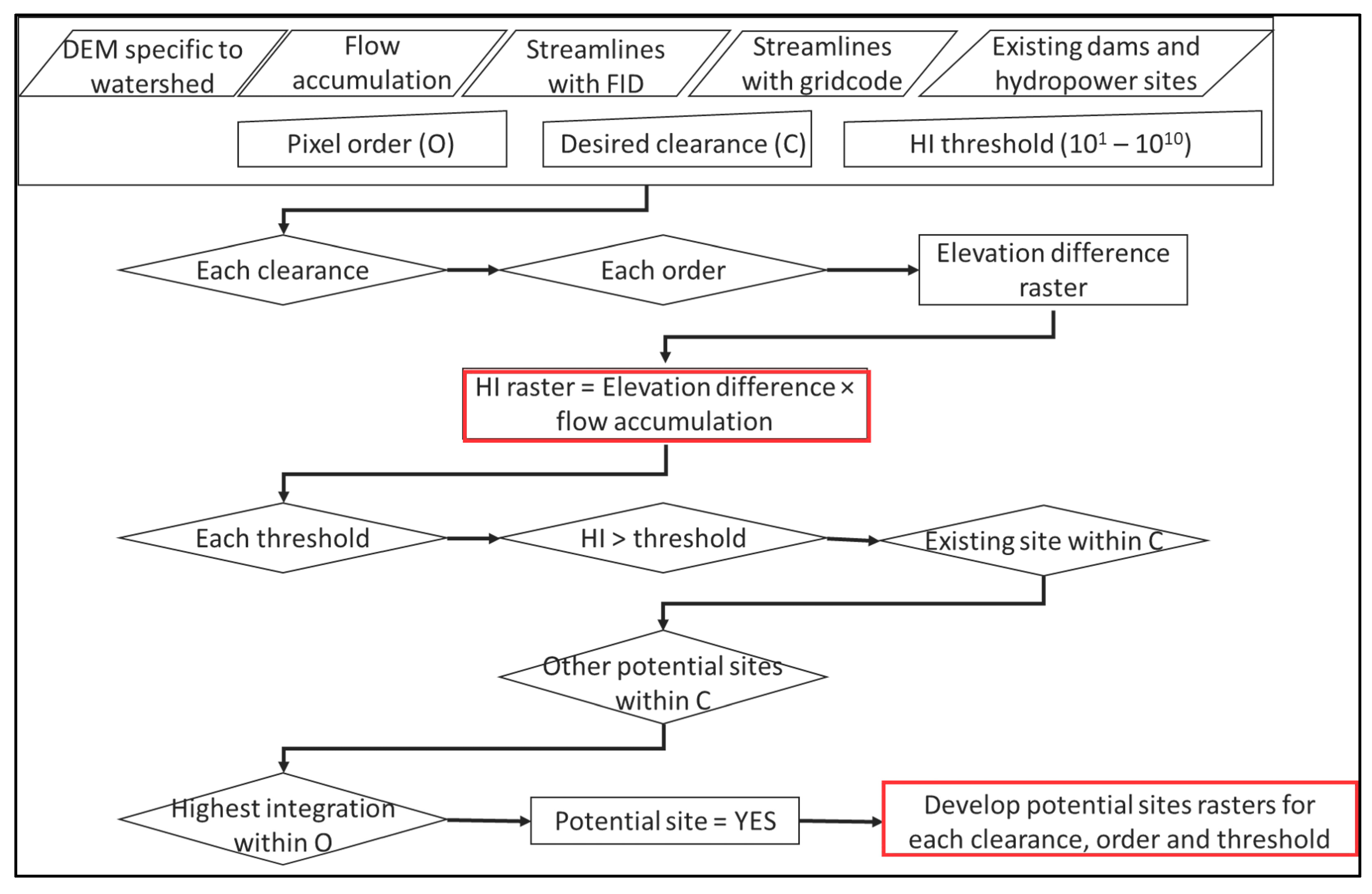
Figure 3 shows the flowchart of the moving window methodology.
We used the PO and combined it with a moving window so each pixel with a streamline would be considered for analysis, the elevation difference being calculated up to 600 m away. This allowed us to obtain high heads for the potential hydropower sites. The code can automatically assume each increasing order between the first and the user-specified order. For example, when we use 20th order for our analysis, the code actually analyzes each order between order 1 ((2 × 1 + 1)2 = 32 pixels) and order 20 ((2 × 20 + 1)2 = 412 pixels) and return the elevation difference raster for each order. This enabled us to perform the sensitivity analysis and determine feasibility of our assumption to divert the flow up to 600 m. The reason we use number 20 specifically is that the SRTM and ASTER have a 30 m spatial resolution, and 600 m distance gives an integer value closer to the diversion of the Rainbow dam. After developing the elevation-difference and HI rasters, we made a MATLAB code to determine the potential hydropower sites. We used a similar moving window, but the order of the window was set in such a way that no two potential sites could be within a certain distance of each other. We call this distance the ‘Clearance’ between two sites. The Clearance is set to ensure that the flow is diverted away from the river flows back to the river safely. To see how Clearance impacts the selection of potential sites, we varied the Clearance from 1 km to 3 km. For Clearance = 1 km, we used a 34th order (1020 m) as the constant order for moving window; and for larger clearances, we multiplied this order by Clearance to obtain new orders. Thus, for Clearance = 2 km, we used 68th order, and for Clearance = 3 km, we used 102nd order. For each value of Clearance, we calculated the potential site for all POs. Additionally, to locate potential sites, we varied the HI value used for assigning a pixel as a potential hydropower site and performed a sensitivity analysis of the variation of the PO and HI. The maximum value of HI (considering both ASTER and SRTM DEM derived hydropower index) was 5.5014 × 10⁹ m for the Morony watershed. Thus, we varied the HI from 101 m to 109 m logarithmically to see how many potential sites were located over each HI threshold in each PO. We used the same methodology with ASTER and SRTM DEMs separately, and for each DEM, 3 values of Clearances, 20 orders and 10 HI thresholds in each order yielded a total of 1200 unique cases for the Morony watershed.
At the same time, we evaluated the performance of the PMMW algorithm by assessing how many of locations of the existing hydropower sites coincided with the predicted potential sites. We downloaded the shapefile of all the existing dams in Montana from Montana Fish and Wildlife Parks (MFWP) website [
44], and all existing and potential hydropower sites in Montana [
45], and clipped them for the Morony Watershed. There are 256 dams and 86 hydropower sites in the watershed. However, there are only 11 hydropower stations with hydropower capacity greater than 5 MW. Since we are interested in locating optimal and large enough hydropower plant sites for economic reasons, we only used these 11 hydropower stations as the existing hydropower sites for model assessment. We also used the locations of two proposed hydropower projects in the watershed ([
46]). In total, we used the locations of 13 existing and proposed hydropower sites for model evaluation. Since the downloaded shapefiles had some discrepancy, we derived our own shapefile by using the data of these projects from various web sources [
46,
54,
55,
56,
57], and coordinates of the dams from Google Earth. Considering the length of dams, pinpointing their exact location is challenging. Therefore, we used the location of upstream of penstocks as the location of hydropower site, since the process of hydropower generation is initiated there. We developed another MATLAB (version R2019a) code with a different moving window to assess the number of locations of potential hydropower sites coinciding with locations of the existing hydropower sites. To prevent the discrepancy in results due to different geographical coordinates of existing and potential hydropower sites, we used the tolerance of 1 km surrounding each existing hydropower site. This means that if any new potential hydropower site location was identified within 1 km of the existing hydropower site location, the model would consider that location as the match between potential and existing hydropower site.
3. Results
We used the ASTER- and SRTM-derived DEMs to determine the elevation difference along each stream line based on the order of the moving window. We used the same DEM to generate the flow accumulation raster. We generated an HI raster to identify potential hydropower sites once the value at a specific location along the streamlines crossed a threshold. We capped the highest possible HI value at 1020 m. The maximum HI values in any integrated raster (considering both ASTER and SRTM DEM derived HI) were 5.5014 × 10⁹ m, and the minimum value of HI was 0. We varied the PO from 1 to 20 to determine the elevation difference between the sites up to 600 m apart, and varied the HI between 101 m and 1010 m. The value of the Clearance was 1 km, 2 km, and 3 km. For each Clearance value, we had 20 orders and 10 thresholds, and therefore, 200 scenarios. Thus, for the three values of Clearance, we had 600 scenarios. Similarly, considering the two DEMs, we had a total of 1200 unique scenarios for the Morony watershed.
To assess the performance of our methodology, we used the number of potential hydropower sites that matched the existing hydropower sites, assuming they were optimized. We developed another MALAB code to determine the number of potential hydropower sites that were within the 1 km vicinity of the locations of existing hydropower plants. Instead of 1 km, we used 1020 m as the distance around existing dams or hydropower sites (due to the 30 m spatial resolution of DEMs) to determine if any potential locations were identified within the specified distance. Then, we performed the sensitivity analysis of all the datasets to determine the preferred values for Clearance, PO, and HI. This assessment analysis was performed for the ASTER- and SRTM-derived DEM datasets separately.
Figure 4 and
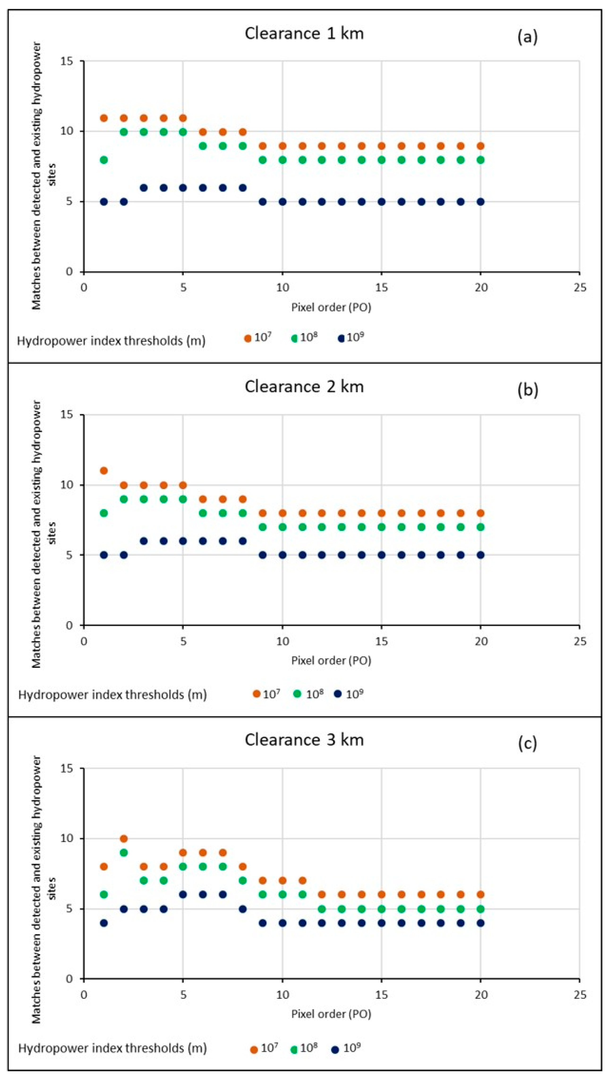
Figure 5 show the assessment analysis of matches between potential hydropower sites and existing dams or hydropower sites within 1020 m clearance for ASTER- and SRTM-derived datasets, respectively. In all the cases, the x axis denotes the PO for the moving window, and the y axis denotes the number of matches between potential and actual hydropower sites. For
Figure 4a (ASTER DEM-derived matches, Clearance = 1 km), the brown, green, and dark blue plots show the number of matches with increasing PO when HI = 10
7 m, 10
8 m, and 10
9 m, respectively. For HI = 10
7 m, when PO = 1, there are 10 matches between actual and potential hydropower sites derived by the model. In both
Figure 4 and
Figure 5, plots for HI = 10
1 m to 10
6 m were excluded because they are nearly identical to the plot for HI = 10
7 m in their respective figures.
For the ASTER-derived DEM data (
Figure 4), for Clearance = 1 km (
Figure 4a), the maximum number of matches between potential and actual hydropower sites was 12. When HI increased to 10
8 m, the number of matches decreased to nine at PO = 9, and was constant afterwards. When HI increased even further to 10
9 m, we had only five matches. For Clearance = 2 km (
Figure 4b), higher HI values yielded even fewer matches. Similar trends continued for the case of Clearance = 3 km (
Figure 4c).
Figure 5 shows similar results to
Figure 4 but for the SRTM DEM data. The general trend of matches was consistent for Clearance = 1 km and 2 km (
Figure 5a,b). The maximum number of matches was 11 when HI = 10
7 m. When Clearance = 3 km (
Figure 5c), maximum matches = 10 and 9 (occurred at PO = 2) for HI = 10
7 m and 10
8 m, respectively. Maximum matches = 6 (occurred at PO = 5–7) for HI = 10
9 m. We can see that for both DEM datasets, lower HI value yielded more matches between potential locations and existing locations, compared to the higher HI values. This is understandable and expected, as higher HI would weed out the sites with lower hydropower capacity. To generate optimal hydropower, we need an HI as high as possible since a larger product of the flow accumulation and head means greater potential to produce hydropower.
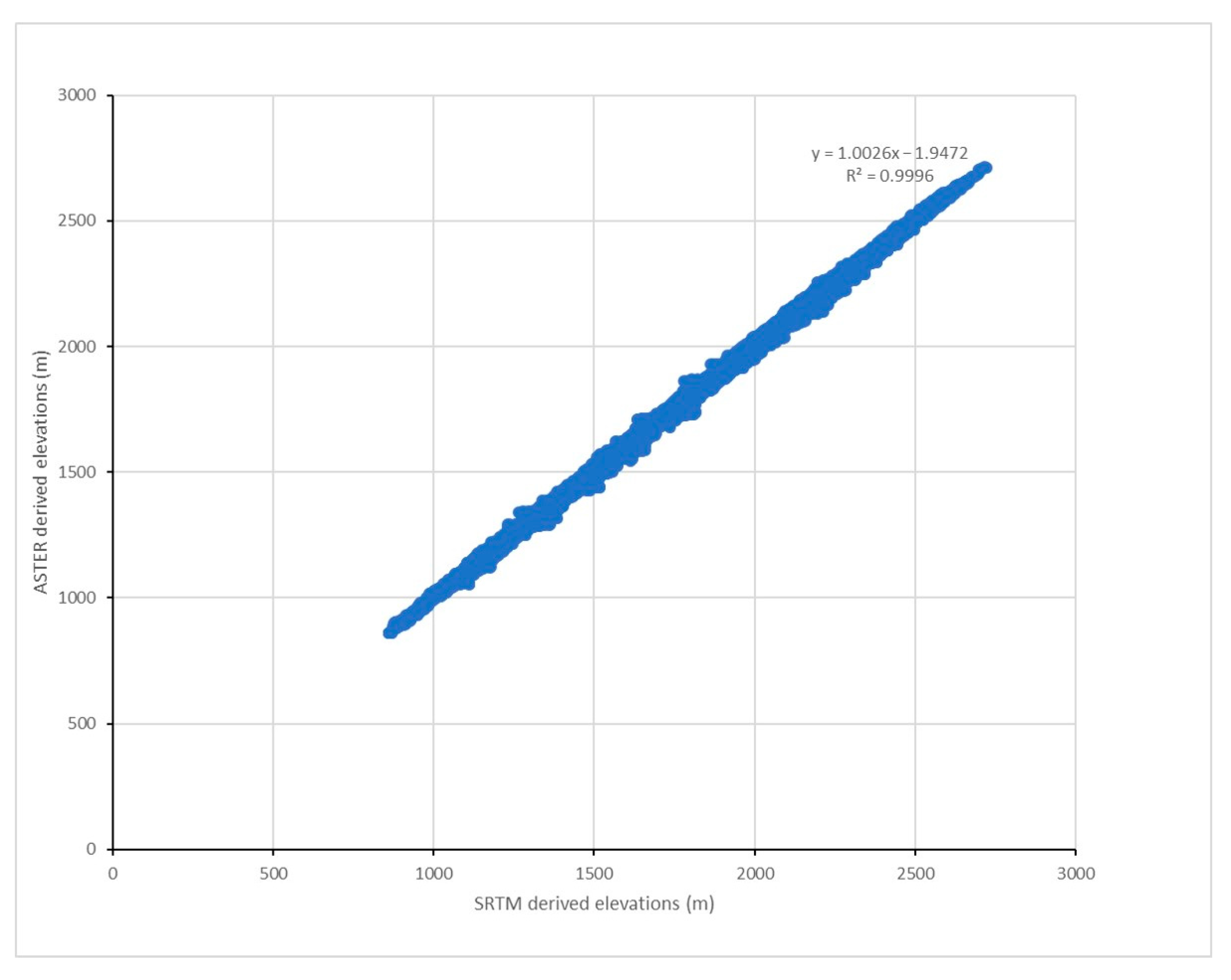
At the same time, we investigated the reason behind the difference observed between the ASTER- and SRTM DEM-derived potential hydropower sites. We performed a regression analysis between the ASTER and SRTM DEMs over streamlines to determine the degree of correlation of elevation over streamlines. The results show that the two DEMs correlated very well, as shown in
Figure 6.
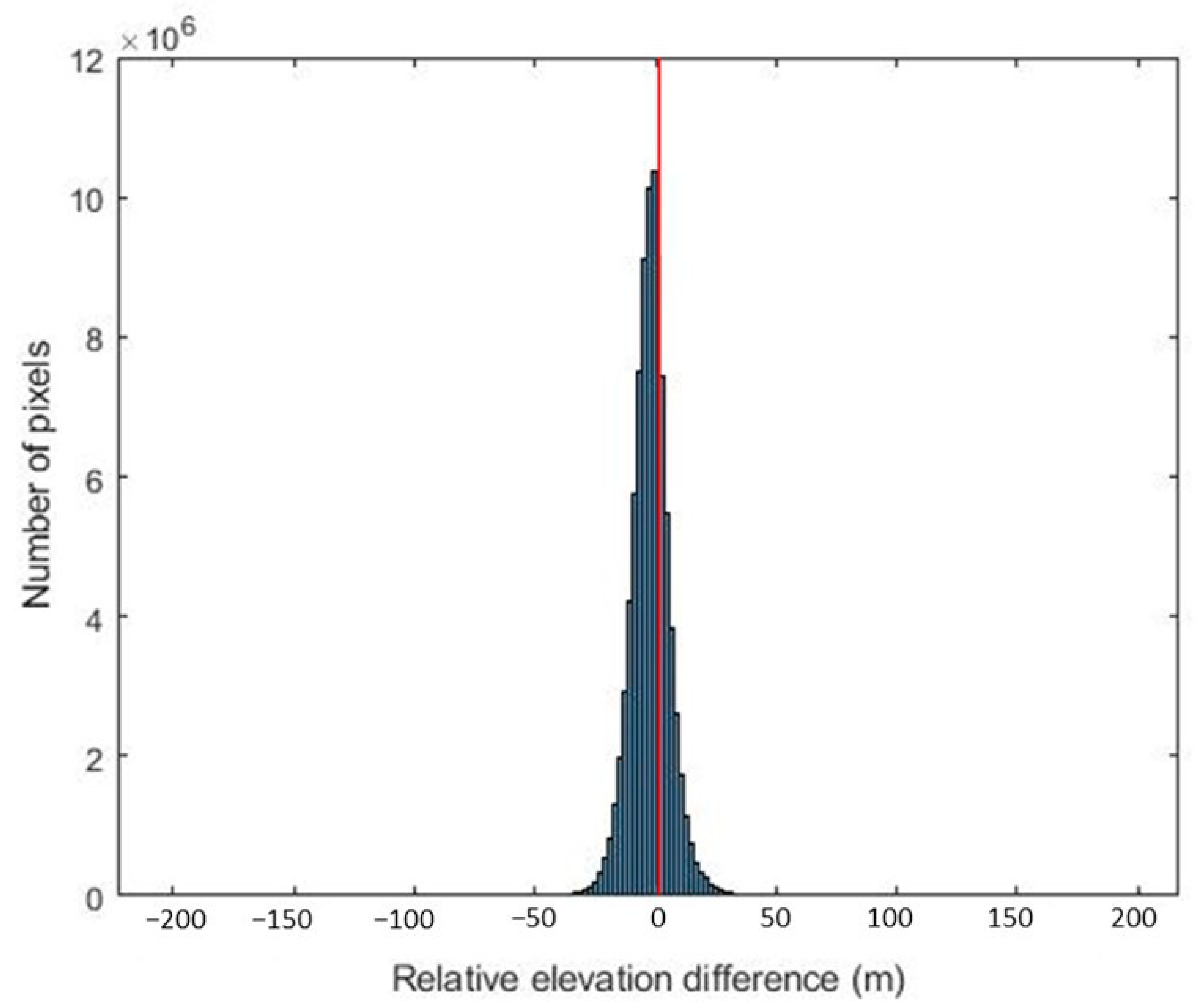
However, we also noticed that because all the elevation values were between 860 m (lowest elevation in watershed) to 3445 m (highest elevation in watershed), the base datum of the region itself was very high. To determine the relative difference between the ASTER and SRTM DEMs, we subtracted the SRTM DEM from the ASTER DEM to determine the relative elevation difference raster of the Morony Watershed, as shown in
Figure 7, and developed a histogram of relative elevation difference, as shown in
Figure 8.
From
Figure 8, we can see that majority of the pixels have a relative elevation difference of less than zero, which indicates that the SRTM DEM has relatively higher elevation values than the ASTER DEM. Since each PO considers (2 × PO + 1)
2 pixels to develop the elevation head and the HI rasters, even smaller relative differences in the ASTER- and SRTM-derived elevations could become the decision making factor for determining the HI at higher POs. We performed a numerical comparison between the HI rasters determined by the various moving orders used in our model. In this comparison, we found that for the two DEMs, the difference between the two HI rasters in each order was significant.
Figure 9 shows the sample results for PO = 3, which was used to determine the potential hydropower sites. We only showed the results of PO = 3 to save space.
4. Discussion
Figure 4 and
Figure 5 show the matches between existing and potential hydropower locations derived via the PMMW model for the ASTER and SRTM datasets, respectively. Since a higher flow accumulation and a larger elevation difference would generate potentially higher hydropower, we only considered HI = 10
7 m or higher to locate potential sites. Based on the trend analysis shown in
Figure 4 and
Figure 5, the trends kept varying with values of Clearance, HI, and PO. Additionally, the ASTER- and SRTM-derived DEM datasets showed difference in the number of potential sites. Therefore, to determine a ‘sweet spot’ of Clearance, PO, and HI, we performed an in-depth assessment of the matches determined between the ASTER- and SRTM-derived datasets for every set of values of Clearance and PO, but only for HI = 10
7 m or higher.
Figure 10 shows the results of the analysis. In each subfigure (
Figure 10a–i), the x-axis indicates the PO, while the y axis indicates the number of matches between the existing and potential hydropower sites. For instance, when the Clearance is 1 km, and the HI is 10
7 m (
Figure 10a), the red and blue plots indicate the number of matches derived from the SRTM and ASTER DEM datasets, respectively.
When Clearance = 1 km and HI = 10
7 m (
Figure 10a), both DEM datasets produced similar number of potential sites as the PO increased. As Clearance increased from 1 km to 3 km, while keeping the HI constant at 10
7 m (
Figure 10a–c: top row), the SRTM DEM dataset generated more matches compared to the ASTER DEM dataset. As HI increased from 10
7 m to 10
9 m, while keeping the Clearance constant at 1 km (
Figure 10a–g: left column), both datasets showed similar matches. As both Clearance and HI increased (
Figure 10a–i: top left to bottom right diagonally), however, SRTM DEM generated more matches than the ASTER DEM. Except for the case of Clearance = 1 km and HI = 10
7 m (
Figure 10a), the SRTM DEM dataset generally identified more matches between potential and existing hydropower sites than the ASTER DEM data. The SRTM DEM dataset seems to function better in locating potential hydropower sites than the ASTER DEM. For this reason, we will use only ASTER DEM for further analysis.
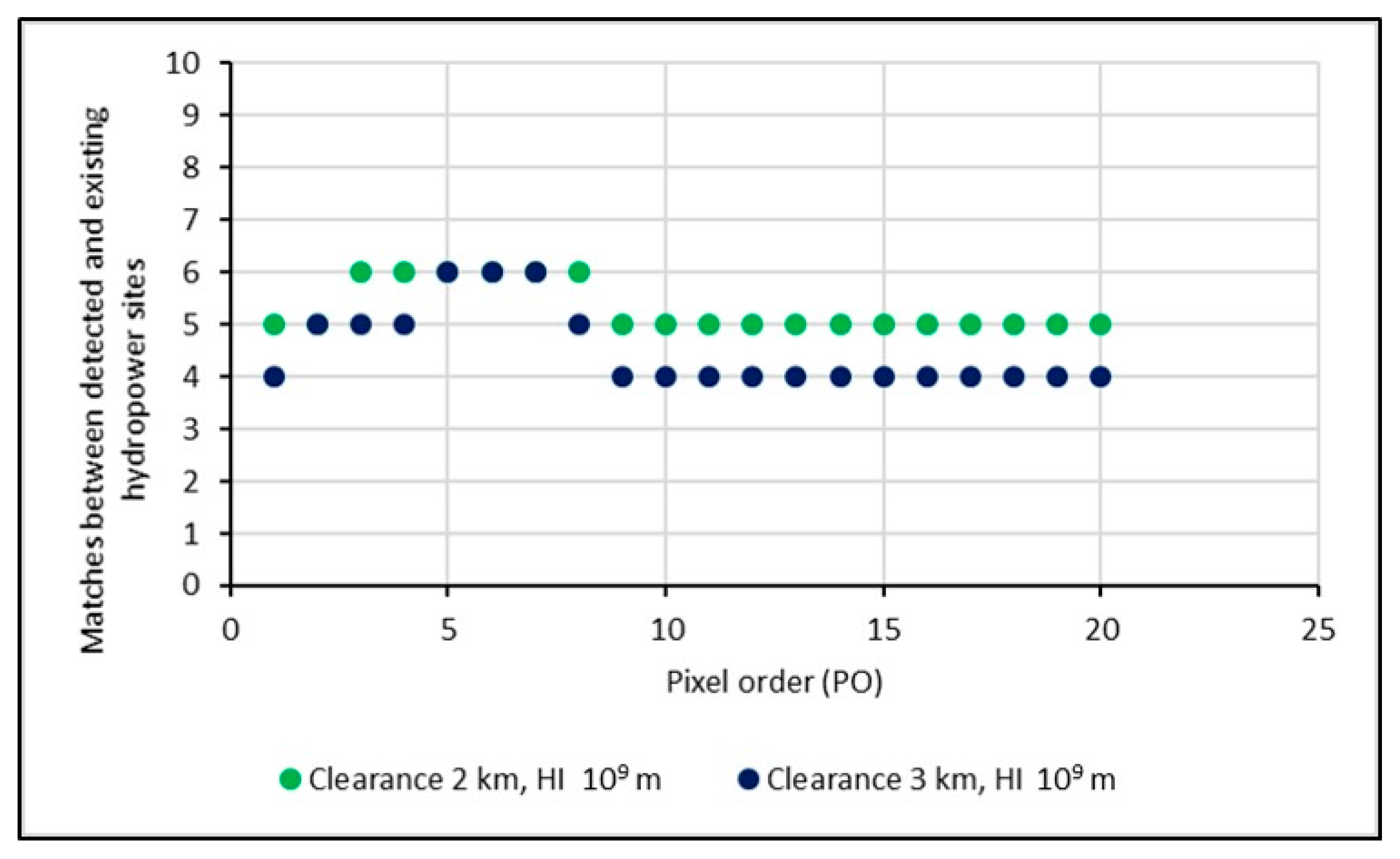
Now let us determine the sweet spot among Clearance, HI, and PO. We only considered the case of HI = 10
9 m and predicted matches for high-capacity potential hydropower sites.
Figure 11 shows the results of matches with increasing PO values for Clearance = 2 km and 3 km. The results for Clearance = 1 km are identical to those for Clearance = 2 km.
From
Figure 11, we can see that a Clearance of 2 km produced six matches between potential and existing hydropower sites when PO = 3. For Clearance = 3 km, the best match of six occurred for PO = 5. We need smaller clearance between dams and smaller diversion for optimal locations. Therefore, Clearance = 1 km with a maximum diversion of 90 m seems optimal for HI = 10
9 m. Considering the 13 locations used to assess the model performance, the model successfully predicted 6 existing locations. However, it should be noted that two of the locations used for the model assessment were proposed hydropower locations, and hydropower plants have not been built yet. Additionally, among the 11 existing hydropower plant sites, only 7 sites had a power output greater than 20 MW. We correlated the potential site locations with existing site locations, and determined that all six matches were of a hydropower station with power output greater than 20 MW (Canyon Ferry—49.8 MW, Black Eagle—21 MW, Rainbow—64 MW, Cochrane—62 MW, Ryan—72, Morony—49 MW). This means that the model predicted six out of seven, i.e., ~86% of the high-energy yielding hydropower sites. Therefore, considering the optimum hydropower potential as the goal, the model accuracy was ~86%.
Table 1 shows the list of the existing hydropower plants with power output greater than 20 MW in the Morony watershed.
Based on the optimum parameters chosen, we derived 12 new potential hydropower sites for the Morony watershed. All of the new potential hydropower sites are over the Upper Missouri River, and downstream of the Canyon Ferry dam for the reason that these locations are close to the watershed outlet at Morony dam, and the elevation change along this segment of the Missouri river is the largest.
Figure 12 shows the potential hydropower sites identified, along with existing locations.
We also performed a polynomial regression analysis between the nominal hydropower output of the six existing hydropower locations that matched the model prediction and HI values corresponding to the six sites. We used the actual power output as a polynomial function of HI (P = f(HI)) to a third order.
Figure 13 shows the regression results between the actual power and the hydropower index. The best-fitting expression is as follows:
where P is the actual power output of the existing hydropower plants, and HI is the Hydropower Index values corresponding to the sites. The coefficient of determination (R
2) of 0.8788 and
p < 0.01 indicates significant correlation. This analysis is very preliminary since the number (six) of hydropower plants over 20 MW along the river is limited.
Based on the curve-fitting regression model (Equation (1)), and upon recalculating the potential hydropower outputs at the six hydropower stations, we noticed that the average projected hydropower output deviated from the actual measurement by up to 11.46%. Assuming the same 11.46% deviation for all 12 newly located potential hydropower sites, we estimated 737.86 MW ± 84.56 MW hydropower output in total, and an average power output of 61.48 MW ± 7.05 MW hydropower output for each newly located hydropower site. It should be noted that the potential hydropower sites were solely based on the optimum head and flow accumulation. The actual construction of a hydropower plant will depend on logistic accessibility, safety, and environmental and other relevant factors. However, using HI as an important parameter in locating potential optimal hydropower sites is a crucial first step, as it is cost-effective, effective, and economic. In addition, the PMMW algorithm only requires DEM of a watershed as input; therefore, it is applicable worldwide since spaceborne remotely sensed DEMs are in the public domain and free-of-charge. Model calibration will be required for each watershed, since the hydrometeorological conditions may vary significantly.
As for the difference between the ASTER and SRTM DEM datasets, from
Figure 9, for PO = 3, a total of (2 × 3 + 1)
2 = 49 pixels were considered to calculate the HI at each center pixel. Therefore, even the small relative elevation differences at a pixel scale in both DEMs can lead to significantly different HI values.


