
A Second-Order Singular Perturbation for Model Simplification for a Microgrid

School of Electrical Engineering and Automation, Anhui University, Hefei 230601, China
*
Author to whom correspondence should be addressed.
Energies 2023, 16(2), 584; https://doi.org/10.3390/en16020584
Submission received: 10 November 2022
/
Revised: 17 December 2022
/
Accepted: 2 January 2023
/
Published: 4 January 2023
(This article belongs to the Section A1: Smart Grids and Microgrids)
Abstract
:As the integration of electronic-interfaced devices have increased, microgrid models have become too complex to perform a stability analysis. Thus, an effective model simplification method keeping most dynamics of the system becomes very essential. Singular perturbation is a common way for model simplification. However, its accuracy is insufficient when nonlinear properties dominate. This is caused by the “Quasi-Steady State Assumption” that traditional singular perturbation holds. By assuming that microgrid can only be stabilized when fast variables stop variating, the traditional method ignores some common phenomena before a stabilization occurs, leading to a loss of dynamics. To improve the accuracy, this paper proposes a “second-order singular perturbation”. Here, the traditional “Quasi-Steady State” is updated to a scenario that third-order derivatives of fast variables become zero before the microgrid stabilizes. The updated assumption covers more common phenomena before a stabilization occurs. This leads to a more precise simplification. Simulation results indicate that the proposed method outperforms traditional singular perturbation in accuracy.
1. Introduction
A microgrid is a small power system integrating renewable generations, electric energy storages and loads [1,2]. Due to the fact that energy storages can adjust their outputs flexibly to compensate the imbalance between generation and consumption [3], microgrids have become an ideal way for the effective utilization of renewable generations with volatile outputs. The ability of keeping stable when encountering a disturbance determines the availability of a microgrid in real operation, and it is quantified via stability analysis. However, as more nonlinear electronic-interfaced devices are integrated into microgrids, making the grid model much more complex than ever, stability analysis of a microgrid has becomes very difficult. Thus, an effective model simplification sustaining a high accuracy makes a stability analysis possible and helps present convincible results.
Various methods for simplifying a microgrid model are reported in recent works in the literature. Kron reduction is a topological simplification approach transforming a complex electrical network into a simple star or triangular formation. This method keeps both static and dynamic performance reliably. In [4], Kron reduction was involved to present a simply topology allowing a separate analysis of inter-inverter oscillating currents. It was proven that the simplified model has a similar dynamic response compared to the original one under small perturbance. Here, “small” means the perturbance mentioned above is unable to change the operation point of the microgrid after stabilization. Kron can sustain a good precision. However, it cannot simplify nonlinear dynamics of electric converters, which is the main cause of grid model complexity, making this method insufficient for stability analysis [5].
Building an equivalent system is also a common way for model simplification. In [6], a simplified model of a microgrid is acquired by combining series or parallel impedances. However, an impedance model is acquired by linearizing the precise model, leading to a lower accuracy. Reference [5] considers multiple microgrids forming a cluster. Microgrids of high concern are kept accurate in the system model, while the others are simplified via structure conservation to form their equivalences. In [7], the virtual synchronous generator (VSG)-controlled microgrid is simplified into a simple synchronous generator, and equivalence error is taken as an extra uncertain parameter for further integration. Building an equivalent system leads to a low calculation burden. However, its parameters are highly affected by the time-varying composition of power system loads and the stochastic behavior of distributed generators. This makes equivalent systems only valid under a certain operating point [8].
Dynamic phasor (DP) is a feature extraction method using Fourier decomposition; it is very suitable for analyzing dynamic properties within various frequency bands. In [9], this method is utilized to build a one-level DP model which is further simplified via first-order Taylor approximation. The authors of reference [10] built a DP model for an unbalanced microgrid and performed a further simplification using a structure-preserving method. DP is well-balanced in accuracy and simplification capability, but decoupling features within different frequency bands may lead to a loss of features concerning frequency coupling. Actually, those coupling features mainly consist of complex and nonlinear properties of electronic-interfaced microgrids.
Other model simplification methods are reported in recent works of the literature, such as dominant-feature extraction in [11], model aggregation in [12] and Takagi–Sugeno modeling in [13].
Singular perturbation is another common way for model simplification. This method focuses on the quasi-steady state of the dynamic system. By picking up several fast state variables and making their derivatives zero, singular perturbation turns those corresponding differential equations into algebraic equations, leading to an order decrement in the model.
In [14], simplification via singular perturbation was conducted on a precise model of three-phase AC microgrids with inverters under voltage and frequency droop controls. Numerical calculation verifies that singular perturbation is quite accurate for small-signal stability analysis. In [15], nonlinear equations of the proposed system were derived in a direct-quadrature reference frame and then linearized around a stable operating point to construct a small-signal model. A reduced-order model consisting of 15 states of the microgrid was derived, compared to the original one with 36 states. Results presented by [16] show the accuracy of singular perturbation for small-signal stability analysis. However, linearization around a certain operating point makes this simplification less precise when analyzing system dynamics under a large perturbation. In [4], the original model was simplified using the same method to analyze oscillation among inverters. Moreover, this order-reduced model is formed to help design control parameters via small-signal stability analysis, which improves the stability of the microgrid significantly [17].
Singular perturbation is well-balanced in simplification capability and accuracy considering the needs of small-signal stability analysis. However, when a large perturbation occurs, leading to a change of operating point, the accuracy of this method seems insufficient [5,11]. This is mainly caused by the traditional “Quasi-Steady States Assumption”, assuming that microgrids can only be stabilized when fast variables stop variating. However, when a microgrid is about to stabilize, there exists phenomena other than a zero-derivative of fast variables. The “Quasi-Steady States Assumption” should be carefully considered when nonlinear properties dominate the microgrid, as its inadequate accuracy may result in a conservative stability assessment.
To solve this problem, this paper proposes a novel model simplification method named “second-order singular perturbation” with a higher accuracy. Here, the traditional “Quasi-Steady State” assumption is updated to the status that third-order derivatives of fast variables turn zero when the microgrid is about to stabilize. The updated assumption describes a scenario that as outer disturbance decreases, microgrids will turn stable when either derivatives or accelerations of fast variables turn zero. It contains more phenomena before a stabilization occurs than the original one does, thus helping improve model accuracy after simplification. Simulation results indicate that this method outperforms the traditional singular perturbation in accuracy.
The structure of this paper is as follows: Section 2 introduces a detailed process of precise modeling for microgrids and the proposed second-order singular perturbation along with its time-separation strategy; Section 3 details parameter setting for simulation and model simplification results concerning the proposed method and a traditional one. Finally, Section 4 presents the conclusion of this paper.
2. Second-Order Singular Perturbation
2.1. Precise Model for a Microgrid
Dynamic properties of a microgrid can be modeled to form a state–space model consisting of N first-order differential equations. Here, variables that provide complete information of the current microgrid condition are named state variables. The way state variables variate are described by the algebraic parts of those differential equations. The state–space model can be presented in the form shown as follows:
Here, x is a vector containing all of the state variables of the microgrid, which represents the current system condition completely. f is a set consisting of continuous differentiable functions representing dynamic relationships among state variables. u is a vector describing the inputs powering the microgrid, such as voltage sources.
Here is an example of a small microgrid containing only a DC energy source connecting a three-phase RLC load through an electronic inverter, as shown in Figure 1. The sequence modeling in the direct-quadrature frame is utilized here, with detailed descriptions presented in [18].
Here, the inverter utilizes inverse droop control with current limiter. Detailed controller configuration is illustrated in Figure 2.
Model of the inverter in positive sequence is shown in Figure 3.
The complete precise model for this microgrid turns out to be 23 orders, which is illustrated as follows:
Here, superscripts 0, 1 and 2 stand for zero, positive and negative components, respectively. Definitions for the 23 state variables are illustrated in Table 1.
2.2. Model Simplification via Singular Perturbation
2.2.1. Timescale Seperation
When a microgrid gradually turns stable after encountering a disturbance, some of its state variables stabilize much more quickly than the others, and they are named “fast variables” and are represented in the form of vector xf here. Due to the fact that fast variables can avoid the influence generated from the other part of the system, they are very independent to system nonlinearity. Thus, state-variable vector x can be divided as follows:
Here, xs refers to the “slow variables” vector containing state variables after xf is excluded.
Then the original model (1) can be transformed into the following form:
2.2.2. Traditional Singular Perturbation
Traditional singular perturbation holds a “Quasi-Steady State” assumption that the microgrid can only be stabilized after derivatives of fast variables turns zero, i.e., they have to stop changing first. Number n + 1 to n + m differential equations in (4) turn into the m algebraic equations shown in (5):
Solving these algebraic equations, we obtain variables xf1, ⋯, xfm presented in the form of algebraic operations among xs1, ⋯, xsn. When they are substituted into (4), the entire model is reduced to n orders rather than the n + m orders that are in the original precise model. However, fast variables ceasing to change is not the only possible phenomenon when a microgrid is about to stabilize. For example, when outer disturbance becomes too small to destabilize the microgrid, the system will turn stable even when fast variables have nonzero derivatives or even nonzero accelerations. This makes the traditional “Quasi-Steady State Assumption” too strict to keep its accuracy.
2.2.3. The Proposed Second-Order Singular Perturbation
In this part, traditional “Quasi-Steady State Assumption” is updated to zero values of third-order derivatives for fast variables. This update describes a situation in which fast variables either stop changing or stop accelerating. Either of the phenomena will definitely occur when a microgrid is about to stabilize.
Firstly, second-order derivatives of xf1, ⋯, xfm are acquired via a further differential calculation on their first derivatives:
Here, can be acquired from the algebraic parts of the first n differential equations in (5). By substituting them into (6), second derivatives of fast variables turn into (7):
Moreover, an extra differential calculation is required to obtain the expression of the third derivative of number i(n + 1 ≤ i ≤ n + m) fast variable, as shown in (8):
Thus, third derivatives of fast variables follow the expressions shown in (9):
By substituting (7) into (8), we obtain full expressions of the third derivatives of fast variables. When they are equal to zero, as shown in (10), the traditional “Quasi-Steady State Assumption” is updated to the scenario in which there is no significant disturbance existing. Thus, this microgrid will stabilize gradually. Of course, this assumption contains the situation that either the derivatives or accelerations are zero.
When the equations in (10) are solved, we can obtain the algebraic expressions of xf1, ⋯, xfm, as shown in (11):
Finally, when (11) is substituted into the first n differential equations of (4), a simplified model of n orders rather than n+m orders are presented in the form of (12):
3. Parameter Setting and Experiment Results
3.1. Parameter Setting
In the microgrid, component parameters and their corresponding are shown in Table 2.
It should be noticed that most of the variables mentioned above can be selected randomly within large ranges. However, some should be chosen carefully to ensure system convergence. For example, Ldc must be set quite small to avoid oscillation of DC voltage. Moreover, a high value of mp or nq leads to significant instability of the microgrid.
Before checking the accuracy of model simplification, initial values should be set to ensure the solvability of differential equations. Each state variable is set to have a zero initial value before the simulation, except for VCdc, of which the initial value VCdc(0) is set to 500 V. Here, VCdc is the voltage on Cdc. The initial values cannot form an equilibrium, indicating that the microgrid was driven off by an outside disturbance before the experiment starts.
3.2. Experiment Results
In the simulation, the proposed method could support various simplification plans, with a maximal five-order-reduction capability, i.e., five state variables are chosen as fast variables and simplified subsequently, as shown in Table 3. Each of these plans leads to identical results as compared to the original precise model. Here, the number and physical meaning for each state variable is illustrated in Table 1 in Section 2.1.
Here, an original precise model and a simplified model delivered by traditional singular perturbation in [17] are selected for comparison to verify the accuracy of the proposed second-order singular perturbation. As each of the plan in Table 3 leads to the same accuracy, the proposed method chooses the first ones, i.e., No. 14, 16, 18, 20 and 22, as fast variables. The traditional method can also support a maximal five-order reduction capability. Among the possible choices, when No. 10, 11, 14, 19 and 23 are selected as fast variables, it leads to a better accuracy.
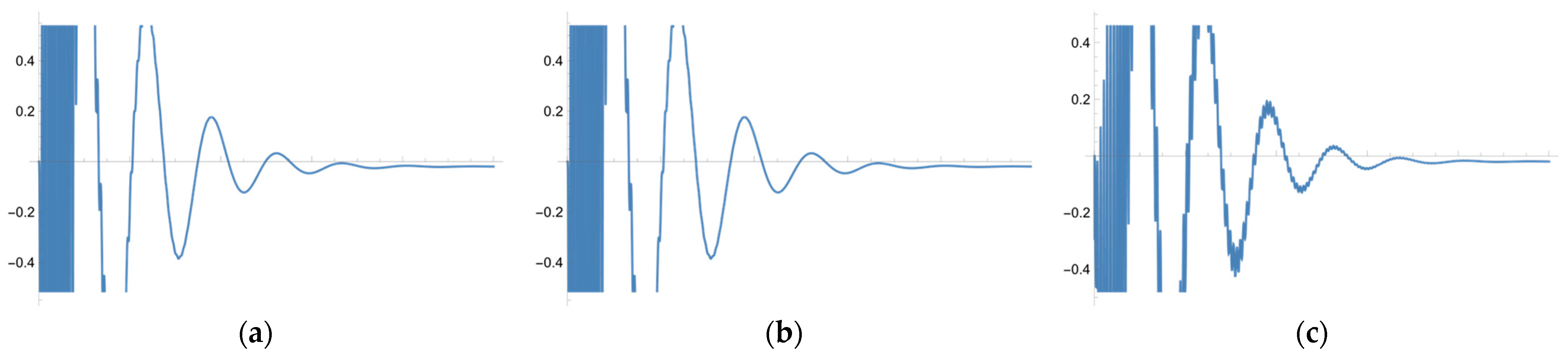
Some state variables solved from three models are as follows: a model simplified using second-order singular perturbation, original precise model and model simplified via traditional singular perturbation; all are presented in Figure 4, Figure 5, Figure 6, Figure 7, Figure 8 and Figure 9. In these figures, variation of the six state variables within 1 s after the microgrid deviates from its original status are illustrated. The physical meanings of these variables can be referred in Table 1 in Section 2.1 via their number in corresponding figure captions. It can be clearly uncovered that the proposed method provides identical results compared to the original model, while traditional singular perturbation is less accurate.
In Figure 4 and Figure 5, Idc(t) and VCdc(t) encounter very small oscillations during the stabilization process for the traditional singular perturbation, as compared to the proposed method and original model. The proposed method precisely keeps the strong coupling of DC and AC parts after simplification, while the traditional method does not.
In Figure 6, active power delivered by the output LCL filter from the three models are presented. This power has no ripple in the results presented by the first two models. On the one hand, ripples become very clear for the traditional method, indicating that it simplifies the ripple restrain function of LCL filter, which is very important for microgrid stabilization capability. This changes output properties of the inverter significantly. On the other hand, the proposed method keeps quite a high precision.
In Figure 7, Figure 8 and Figure 9, , and solved from the model generated by traditional method differ from the proposed method and the original model both in ripples and oscillation magnitude. These states describe the output current of the inverter and LCL filter. System stabilization features are simplified via the traditional method; apparently, this will lead to inaccurate results for stability analysis. Thus, it can be concluded that the second-order singular perturbation keeps accurate dynamics of the filter and stabilization features of the whole microgrid.
4. Conclusions
Microgrids have become an ideal way for effective utilization of renewable generations with volatile outputs. However, more integration of nonlinear electronic-interfaced devices makes the model of microgrids too complex to perform a stability analysis. Thus, an effective model simplification method sustaining high precision is very essential. Singular perturbation is a common way for model simplification. However, its accuracy is insufficient when nonlinear properties dominate. This is caused by the “Quasi-Steady State Assumption” assuming that microgrids can only be stabilized when fast variables stop variating, leading to the ignorance of some common phenomena before a stabilization occurs and to a loss of dynamics.
To improve the simplification accuracy, this paper proposes a “second-order singular perturbation” method. Here, the traditional “Quasi-Steady State” is updated to a scenario that third-order derivatives of fast variables become zero before the microgrid stabilizes. This assumption turns to the assumption that as outer disturbance decreases, the microgrid will turn stable even when derivatives or accelerations of fast variables are nonzero. The updated assumption contains common phenomena before a stabilization occurs. Simulation results indicate that this method outperforms the traditional singular perturbation in accuracy. Simplification capability of the proposed method makes a stability analysis possible. On the other hand, higher accuracy of this method helps present a more convincible result for stability analysis.
Author Contributions
Conceptualization, investigation, methodology, software, writing—original draft and writing—review and editing, X.-Q.Y.; validation and visualization, X.-Q.Y. and B.-S.Y.; supervision, J.T. All authors have read and agreed to the published version of the manuscript.
Funding
This work was supported in part by the National Natural Science Foundation of China under Grant 52207072 and in part by the Anhui Education Department Research Project under Grant KJ2020A0029.
Data Availability Statement
Not applicable.
Conflicts of Interest
The authors declare no conflict of interest.
References
- Sun, L.; Zhao, X.; Lv, Y. Stability Analysis and Performance Improvement of Power Sharing Control in Islanded Microgrids. IEEE Trans. Smart Grid 2022, 13, 4665–4676. [Google Scholar] [CrossRef]
- Abdelgabir, H.; Shaheed, M.N.B.; Elrayyah, A.; Sozer, Y. A Complete Small-Signal Modelling and Adaptive Stability Analysis of Nonlinear Droop-Controlled Microgrids. IEEE Trans. Ind. Appl. 2022, 58, 7620–7633. [Google Scholar] [CrossRef]
- Xu, Y.; Chen, X.; Zhang, H.; Yang, F.; Tong, L.; Yang, Y.; Yan, D.; Yang, A.; Yu, M.; Liu, Z.; et al. Online Identification of Battery Model Parameters and Joint State of Charge and State of Health Estimation Using Dual Particle Filter Algorithms. Int. J. Energy Res. 2022, 46, 19615–19652. [Google Scholar] [CrossRef]
- Nikolakakos, I.P.; Zeineldin, H.H.; El-Moursi, M.S.; Kirtley, J.L. Reduced-Order Model for Inter-Inverter Oscillations in Islanded Droop-Controlled Microgrids. Ieee Trans. Smart Grid 2018, 9, 4953–4963. [Google Scholar] [CrossRef]
- Shuai, Z.; Peng, Y.; Liu, X.; Li, Z.; Guerrero, J.M.; Shen, Z.J. Dynamic Equivalent Modeling for Multi-Microgrid Based on Structure Preservation Method. IEEE Trans. Smart Grid 2019, 10, 3929–3942. [Google Scholar] [CrossRef]
- Rashidirad, N.; Hamzeh, M.; Sheshyekani, K.; Afjei, E. A Simplified Equivalent Model for the Analysis of Low-Frequency Stability of Multi-Bus DC Microgrids. IEEE Trans. Smart Grid 2018, 9, 6170–6182. [Google Scholar] [CrossRef]
- Hu, W.; Wu, Z.; Lv, X.; Dinavahi, V. Robust Secondary Frequency Control for Virtual Synchronous Machine-Based Microgrid Cluster Using Equivalent Modeling. IEEE Trans. Smart Grid 2021, 12, 2879–2889. [Google Scholar] [CrossRef]
- Kontis, E.O.; Papadopoulos, T.A.; Syed, M.H.; Guillo-Sansano, E.; Burt, G.M.; Papagiannis, G.K. Artificial-Intelligence Method for the Derivation of Generic Aggregated Dynamic Equivalent Models. IEEE Trans. Power Syst. 2019, 34, 2947–2956. [Google Scholar] [CrossRef] [Green Version]
- Levron, Y.; Belikov, J. Modeling Power Networks Using Dynamic Phasors in the Dq0 Reference Frame. Electr. Power Syst. Res. 2017, 144, 233–242. [Google Scholar] [CrossRef]
- Wang, H.; Jiang, K.; Shahidehpour, M.; He, B. Reduced-Order State Space Model for Dynamic Phasors in Active Distribution Networks. IEEE Trans. Smart Grid 2020, 11, 1928–1941. [Google Scholar] [CrossRef]
- Yu, H.; Su, J.; Wang, H.; Wang, Y.; Shi, Y. Modelling Method and Applicability Analysis of a Reduced-Order Inverter Model for Microgrid Applications. IET Power Electron. 2020, 13, 2638–2650. [Google Scholar] [CrossRef]
- Taul, M.G.; Wang, X.; Davari, P.; Blaabjerg, F. Reduced-Order and Aggregated Modeling of Large-Signal Synchronization Stability for Multiconverter Systems. IEEE J. Emerg. Sel. Top. Power Electron. 2021, 9, 3150–3165. [Google Scholar] [CrossRef]
- Liu, S.; Li, X.; Xia, M.; Qin, Q.; Liu, X. Takagi-Sugeno Multimodeling-Based Large Signal Stability Analysis of DC Microgrid Clusters. IEEE Trans. Power Electron. 2021, 36, 12670–12684. [Google Scholar] [CrossRef]
- Mariani, V.; Vasca, F.; Vásquez, J.C.; Guerrero, J.M. Model Order Reductions for Stability Analysis of Islanded Microgrids With Droop Control. IEEE Trans. Ind. Electron. 2015, 62, 4344–4354. [Google Scholar] [CrossRef] [Green Version]
- Rasheduzzaman, M.; Mueller, J.A.; Kimball, J.W. Reduced-Order Small-Signal Model of Microgrid Systems. IEEE Trans. Sustain. Energy 2015, 6, 1292–1305. [Google Scholar] [CrossRef]
- Vorobev, P.; Huang, P.; Hosani, M.A.; Kirtley, J.L.; Turitsyn, K. High-Fidelity Model Order Reduction for Microgrids Stability Assessment. IEEE Trans. Power Syst. 2018, 33, 874–887. [Google Scholar] [CrossRef] [Green Version]
- Eberlein, S.; Rudion, K. Small-Signal Stability Modelling, Sensitivity Analysis and Optimization of Droop Controlled Inverters in LV Microgrids. Int. J. Electr. Power Energy Syst. 2021, 125, 106404. [Google Scholar] [CrossRef]
- Roos, M.H.; Nguyen, P.H.; Morren, J.; Slootweg, J.G. Direct-Quadrature Sequence Models for Energy-Function Based Transient Stability Analysis of Unbalanced Inverter-Based Microgrids. IEEE Trans. Smart Grid 2021, 12, 3692–3704. [Google Scholar] [CrossRef]
Figure 1.
The microgrid tested in this paper.

Figure 2.
Inverse droop control utilized in the inverter.

Figure 3.
Model of the inverter in positive sequence.
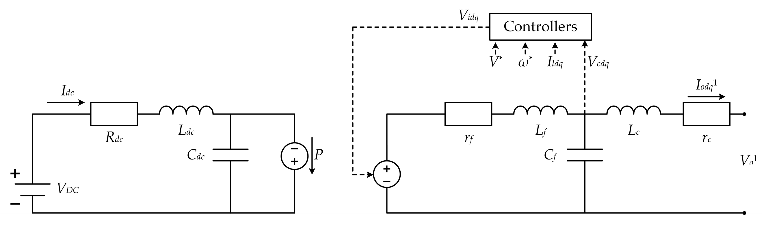
Figure 4.
No. 1 state variable Idc(t) solved from the 3 models. (a) Result from the proposed method, (b) Result from the original precise model. (c) Result from the traditional singular perturbation.
Figure 4.
No. 1 state variable Idc(t) solved from the 3 models. (a) Result from the proposed method, (b) Result from the original precise model. (c) Result from the traditional singular perturbation.

Figure 5.
No. 2 state variable VCdc(t) solved from the 3 models. (a) Result from the proposed method, (b) Result from the original precise model. (c) Result from the traditional singular perturbation.
Figure 5.
No. 2 state variable VCdc(t) solved from the 3 models. (a) Result from the proposed method, (b) Result from the original precise model. (c) Result from the traditional singular perturbation.
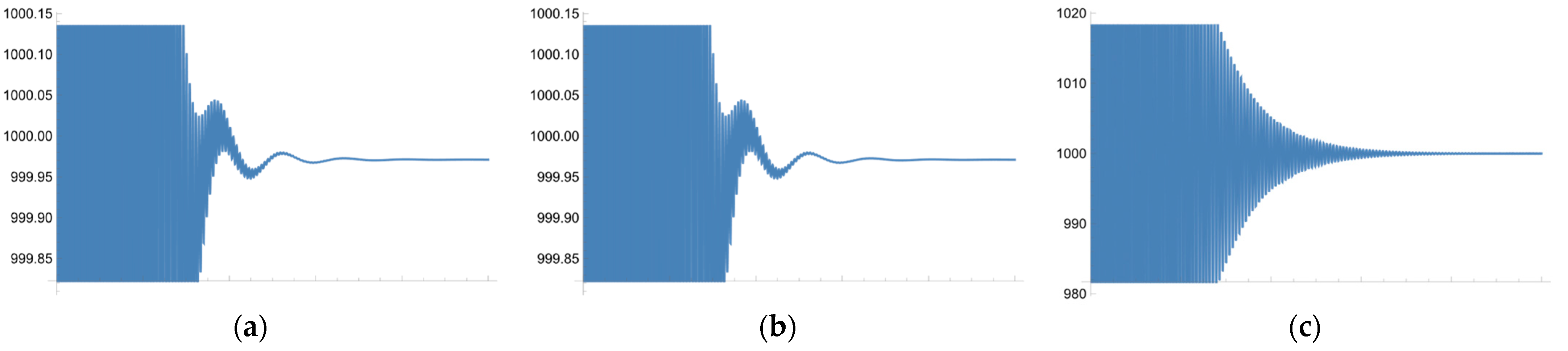
Figure 6.
No. 4 state variable P1(t) solved from the 3 models. (a) Result from the proposed method, (b) Result from the original precise model. (c) Result from the traditional singular perturbation.
Figure 6.
No. 4 state variable P1(t) solved from the 3 models. (a) Result from the proposed method, (b) Result from the original precise model. (c) Result from the traditional singular perturbation.
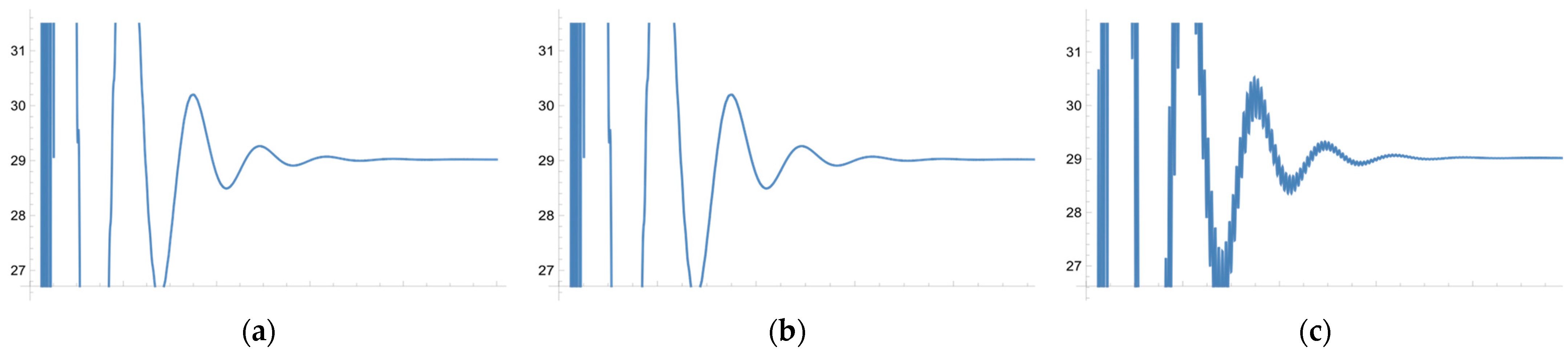
Figure 7.
No. 10 state variable solved from the 3 models. (a) Result from the proposed method, (b) Result from the original precise model. (c) Result from the traditional singular perturbation.
Figure 7.
No. 10 state variable solved from the 3 models. (a) Result from the proposed method, (b) Result from the original precise model. (c) Result from the traditional singular perturbation.
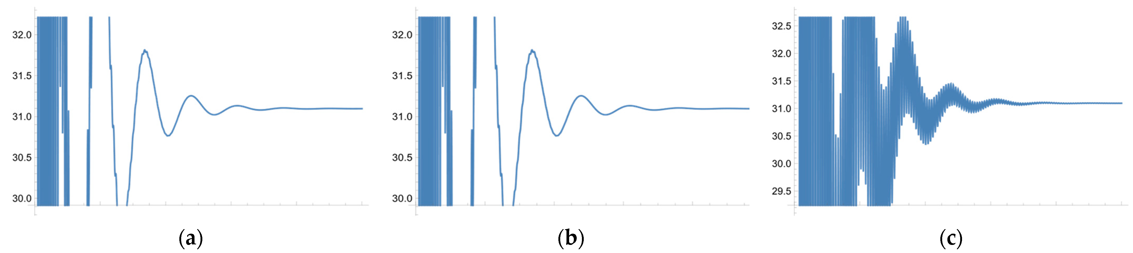
Figure 8.
No. 11 state variable solved from the 3 models. (a) Result from the proposed method, (b) Result from the original precise model. (c) Result from the traditional singular perturbation.
Figure 8.
No. 11 state variable solved from the 3 models. (a) Result from the proposed method, (b) Result from the original precise model. (c) Result from the traditional singular perturbation.
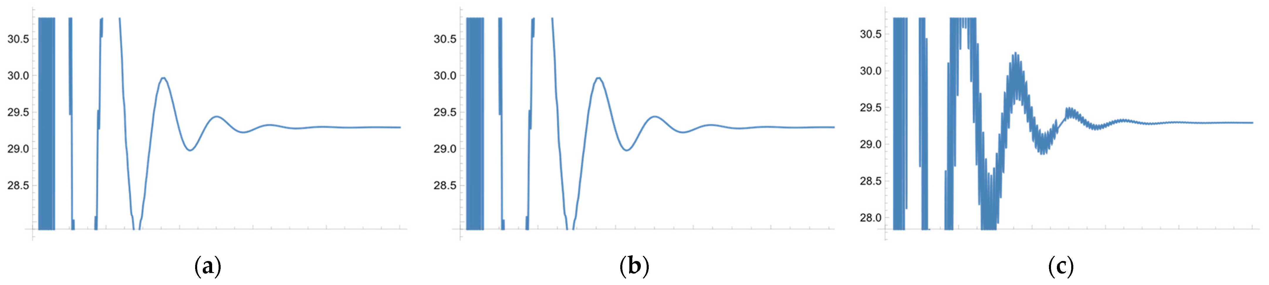
Figure 9.
No. 15 state variable solved from the 3 models. (a) Result from the proposed method, (b) Result from the original precise model. (c) Result from the traditional singular perturbation.
Figure 9.
No. 15 state variable solved from the 3 models. (a) Result from the proposed method, (b) Result from the original precise model. (c) Result from the traditional singular perturbation.

Table 1.
Number and definition for each state variable.
| Number | Variable | Definition |
|---|---|---|
| 1 | Idc | Current of DC side |
| 2 | VCdc | Voltage on the capacitor of DC side |
| 3 | θ | Angle of the inverter |
| 4 | P1 | Output active power after the LCL filter |
| 5 | Q1 | Output reactive power after the LCL filter |
| 6 (7) | Intermediate Variable | |
| 8 (9) | AC output current deviation from its nominal in positive sequence and d(q) frame | |
| 10 (11) | Positive-sequence component of inverter output current in positive sequence and d(q) frame | |
| 12 (13) | Voltage on the capacitor of LCL filter in positive sequence and d(q) frame | |
| 14 (15) | Output current of the LCL filter in positive sequence and d(q) frame | |
| 16 (17) | Voltage on the capacitor of LCL filter in zero sequence and d(q) frame | |
| 18 (19) | Output current of the LCL filter in zero sequence and d(q) frame | |
| 20 (21) | Voltage on the capacitor of LCL filter in negative sequence and d(q) frame | |
| 22 (23) | Output current of the LCL filter in negative sequence and d(q) frame |
Table 2.
Component parameters and their definitions of the microgrid.
| Variable | Value | Definition |
|---|---|---|
| Vtri | 1 V | Peak amplitude of the triangular signal of the PWM drive circuit |
| Rdc | 0.002 | Resistance at the DC side |
| rf | 0.001 | Input resistance of the LCL filter |
| Ldc | 2 mH | Equivalent inductance of the DC side |
| Lf | 15 mH | Input inductance of the LCL filter |
| Lc | 20 μH | Output inductance of the LCL filter |
| Cdc | 680 μF | Equivalent capacitor of the DC side |
| Cf | 300 μF | Capacitor of LCL filter |
| VDC | 1000 V | Output voltage of the DC source |
| V* | 311 V | Nominal output voltage of the inverter (amplitude) |
| ω* | 314 | Nominal output angular frequency of the inverter |
| Kic(Kpc) | 0.02 () | Current (power) gains of current controller |
| Kiv(Kpv) | 200 (0.2) | Current (power) gains of voltage controller |
| mp(nq) | P-V (Q-) droop coefficient |
Table 3.
Available simplification plan with 5 fast variables for the proposed method.
| Variable Combination to Be Simplified | Variable Combination to Be Simplified |
|---|---|
| 14, 16, 18, 20, 22 | 15, 16, 18, 20, 22 |
| 14, 16, 18, 20, 23 | 15, 16, 18, 20, 23 |
| 14, 16, 18, 21, 23 | 15, 16, 18, 21, 23 |
| 14, 16, 19, 20, 22 | 15, 16, 19, 20, 22 |
| 14, 16, 19, 20, 23 | 15, 16, 19, 20, 23 |
| 14, 16, 19, 21, 22 | 15, 16, 19, 21, 22 |
| 14, 16, 19, 21, 23 | 15, 16, 19, 21, 23 |
| 14, 17, 18, 20, 23 | 15, 17, 18, 20, 23 |
| 14, 17, 18, 21, 22 | 15, 17, 18, 21, 22 |
| 14, 17, 18, 21, 23 | 15, 17, 18, 21, 23 |
| 14, 17, 19, 20, 22 | 15, 17, 19, 20, 22 |
| 14, 17, 19, 20, 23 | 15, 17, 19, 20, 23 |
| 14, 17, 19, 21, 22 | 15, 17, 19, 21, 22 |
| 14, 17, 19, 21, 23 | --- |
Disclaimer/Publisher’s Note: The statements, opinions and data contained in all publications are solely those of the individual author(s) and contributor(s) and not of MDPI and/or the editor(s). MDPI and/or the editor(s) disclaim responsibility for any injury to people or property resulting from any ideas, methods, instructions or products referred to in the content. |
© 2023 by the authors. Licensee MDPI, Basel, Switzerland. This article is an open access article distributed under the terms and conditions of the Creative Commons Attribution (CC BY) license (https://creativecommons.org/licenses/by/4.0/).
Share and Cite
MDPI and ACS Style
Yin, X.-Q.; Yang, B.-S.; Tao, J. A Second-Order Singular Perturbation for Model Simplification for a Microgrid. Energies 2023, 16, 584. https://doi.org/10.3390/en16020584
AMA Style
Yin X-Q, Yang B-S, Tao J. A Second-Order Singular Perturbation for Model Simplification for a Microgrid. Energies. 2023; 16(2):584. https://doi.org/10.3390/en16020584
Chicago/Turabian StyleYin, Xiao-Qi, Bao-Shun Yang, and Jun Tao. 2023. "A Second-Order Singular Perturbation for Model Simplification for a Microgrid" Energies 16, no. 2: 584. https://doi.org/10.3390/en16020584
Note that from the first issue of 2016, this journal uses article numbers instead of page numbers. See further details here.