
A Stochastic Model of Anomalously Fast Transport of Heat Energy in Crystalline Bodies

Department of Mathematics, Lublin University of Technology, Nadbystrzycka 38, 20-618 Lublin, Poland
*
Author to whom correspondence should be addressed.
Energies 2023, 16(20), 7117; https://doi.org/10.3390/en16207117
Submission received: 11 September 2023
/
Revised: 10 October 2023
/
Accepted: 11 October 2023
/
Published: 17 October 2023
(This article belongs to the Topic Thermal Energy Transfer and Storage)
Abstract
:In this work, a new method for constructing the infinite-dimensional Ornstein–Uhlenbeck stochastic process is introduced. The constructed process is used to perturb the harmonic system in order to model anomalously fast heat transport in one-dimensional nanomaterials. The introduced method made it possible to obtain a transition probability function that allows for a different approach to the analysis of equations with such a disturbance. This creates the opportunity to relax assumptions about temporal correlations for such a process, which may lead to a qualitatively different model of energy transport through vibrations of the crystal lattice and, as a result, to obtain the superdiffusion equation on a macroscopic scale with an order of the fractional Laplacian different from the value of 3/4 obtained so far in stochastic models. Simulations confirming these predictions are presented and discussed.
1. Introduction
Thermal conductivity in nanomaterials is an extremely interesting research area in the field of nanotechnology and materials science. In our work, we deal with modeling heat flow in one-dimensional crystalline bodies, for example nanowires. So, let us focus our attention on such materials and briefly describe the possibilities of their use. Metallic nanowires have unique thermal conductivity properties due to their small size and structure. Research on metallic nanowires and their properties such as electrical and thermal conductivity began in full force at the turn of the 20th and 21st centuries, and many research works and experiments have been conducted since then. The study of thermal conductivity in metallic nanowires is important for both scientific and practical reasons. They could help design more efficient thermoelectric materials that convert heat into electricity, and develop advanced thermal materials used in electronics, nanotechnologies, energy technology, and more.
The phenomenon of thermal superconductivity in model of one-dimensional crystalline body was first observed by Lepri, Livi, and Politi, and described in [1]. In this paper, the system of equations describing the vibrations of coupled nonlinear oscillators was solved numerically and the divergence of thermal conductivity was demonstrated. The importance of this research is underlined in review work [2], where the authors write: “This marked the beginning of a research endeavor that, over more than two decades, has been devoted to understanding the mechanisms giving rise to anomalous transport in low-dimensional systems. Far from being a purely academic exercise, this research has unveiled the possibility of observing such peculiar effects in nanomaterials, such as nanotubes, nanowires, or graphene [3,4]”. Since then, research into physical and mathematical models has continued [5,6,7,8,9,10,11]. A significant voice in the ongoing discussion was the article [12], in which a stochastic disturbance preserving energy and momentum was introduced into the harmonic model. The authors pointed out the important role of the law of momentum conservation in the anomalous thermal conductivity. The next step was made in the work [13], where the authors have shown that the microscopic dynamics, introduced in [12], satisfy the linear Boltzmann equation for phonons on the mesoscopic scale. In turn, the works [14] and [15] show that the solution of the Boltzmann equation scaled to the macroscopic scale satisfies the superdiffusion equation with an order of the fractional Laplacian equal to . Subsequently, in [16], a direct transition from the microscopic model to the macroscopic superdiffusion equation was made. In [17], the same authors modified the stochastic perturbation, introduced in [12], by replacing the Gaussian noise with the Ornstein–Uhlenbeck process, then obtained the linear Boltzmann equation at the mesoscopic scale.
All stochastic models discussed led to the same superdiffusion equation. This work paves the way to obtain the superdiffusion equation with a different order of fractional Laplacian. Namely, we construct the stochastic disturbance in a different way and present a proposal, supported by simulations, on how to transform the microscopic model into a macroscopic model to achieve the intended research goal.
Despite the utilization of highly advanced mathematical techniques, our intention is to communicate this research to a community primarily focused on experimental investigations. Our underlying belief is that fostering an exchange of research methods between these two groups of researchers may yield mutual benefits, potentially leading to collaborations that unveil new perspectives and avenues of exploration.
In the following part of the introduction, we discuss the construction of the model, introducing the reader to the topic.
1.1. Stochastic Models of Heat Transport
In insulating solids thermal energy is carried out by lattice vibrations propagating through the material. This is also the main medium of heat transfer in semiconductors [18]. On a microscopic scale, energy is transmitted by the interactions of neighboring atoms. We focus on the one-dimensional model. The equilibrium positions of atoms are denoted by integers x. The deflection from the equilibrium position of the atom at site x is denoted by and its momentum by . Its total energy is
where is the kinetic energy, and W, V are potentials, wherein V depends only on relative positions of adjacent atoms [19,20]. The atom transmits energy to its neighbors through elastic bonds—see Figure 1.
The wave propagating along the chain can be decomposed into sinusoidal oscillations with a specific direction of propagation—called normal modes. Each normal mode is labeled by number k, which belongs to the interval . Endpoints and are identified, as they represent the same normal mode—the sinusoidal wave with wavelength equal to , where is the distance between equilibrium positions of two adjacent oscillators (see Figure 1). In this normal mode, every pair of two adjacent atoms oscillate in the counterphase. If , then k and denote waves of the same space length , but traveling in the opposite directions along the chain (Figure 2).
Total energy of the system decomposes into normal mode energies
We will be always assuming that potential W in (1) is zero, as this is the case when anomalous heat transport appears in dimension one. Let us for a moment assume that V is quadratic, for some . The model is then linear and oscillators are harmonic. For convenience, we set . Now, (1) takes the form
Hamilton’s equations derived from (2) are
see [21] on p. 6. In this case, each normal mode k has the phase velocity
see [22] on p. 68-69 for the derivation. The function is called dispersion relation. The group velocity for a wave packet (Figure 3) is specified by the derivative , see [23] on p. 47.
After proper space-time rescaling of the dynamics of energy propagation given by (3), we obtain the linear transport equation at the mesoscopic scale (see Figure 4)
Here, the function has physical interpretation of the energy density of the normal mode at space coordinate at time instant t. Heuristically, according to (4), if a quantum of energy is carried by normal mode k, then it travels ballistically along the chain at constant velocity . It also stays in this mode forever.
If we further rescale the dynamics in space and time in attempt to obtain to the macroscopic scale, the speed of energy propagation approaches infinity, which is nonsense in the context of heat propagation, thus the assumption that oscillators are harmonic (V is quadratic) does not work in modeling heat transfer. On the other hand, if the potential V has the form
where is a nonzero non-quadratic term (see i.g. classical FPU model [24,25]) then the study of the model encounters major analytical difficulties. Therefore, mathematical physicists are interested in probabilistic models in which , but the dynamics of harmonic oscillators is randomly disturbed. Stochastic, time-dependent processes are introduced into the equations to mimic the chaos occurring in deterministic non-linear models. With this approach, the dynamics (3) is altered in the following manner:
where , is a sequence of stochastic processes. Such models result in the linear Boltzmann equation at the mesoscopic scale ([13], p. 172). Compare it with Equation (4).
Here, is a scattering operator acting on the variable k. In a heuristic description the appearance of means, that—in opposition to the harmonic case—different normal modes interact and exchange energy. A quantum of energy absorbed by a normal mode is in this context called phonon. We will say that phonon is in the state when it is absorbed by mode . Being in the state , the phonon propagates with velocity until it is intercepted (at a random time instant) by a (random) mode and changes its velocity to —and so on. In this description, we perceive the thermal energy of the medium as a cloud of quasiparticles—phonons—traveling in this way. The dynamics of this cloud at the macroscopic scale gives us the heat equation.
We recall the classical heat (diffusion) equation:
where c is a positive constant, are time and space coordinates, and is the Laplacian operator acting on x. Microscopic mathematical models try to capture the fact that observed heat propagation does not always satisfy the above equation. The phenomenon of anomalous, super-diffusive heat flow is observed numerically and experimentally in one dimensional nanomaterials. It is described by superdiffusion equation
where is a parameter and is the fractional Laplacian. In recent years, many articles have been published devoted to understanding such unusual heat propagation.
1.2. Classical and Anomalous Heat Transport
As we indicated above, the Boltzmann Equation (7) is related to a stochastic process describing the motion of a phonon traveling with the velocity , wherein its state k, and consequently its velocity, changes randomly at random time instants. More specifically, the scattering operator has the form
The function , called collision kernel, determines the probability that a phonon in a state k will go to a state , and the average time the particle stays in any state k. We emphasize the following facts:
- (a)
- The shape of the kernel, hence the parameters of phonon trajectories, emerges from the stochastic perturbation put into microscopic dynamics (6);
- (b)
- The shape of the kernel determines type of heat transport at the macroscopic scale.
We elaborate point (b): if the trajectories of phonons are asymptotically diffusive, then the heat transport satisfies classical heat Equation (8). However, we can deal with models in which some normal modes weakly interact with other modes, which has an effect on a macroscopic scale. A phonon that has fallen into such a normal mode travels in ballistic motion for a relatively long time before it falls out of it and its trajectory becomes diffusive again, and these ballistic parts of the trajectory make heat transfer anomalously fast.
In the model introduced in [12,19] the stochastic perturbation of microscopic dynamics is spatially and temporally uncorrelated—it is a Gaussian noise, i.e., , of (6) is a family of independent Brownian motions. This model reproduces anomalous heat transport in the one dimensional chain, which agrees with observations. The collision kernel obtained for this one-dimensional model is
where
The heat transport related to the model satisfies Equation (9) with . Mathematically, this value of results from the fact that the function , defined as
is asymptotically similar to as . The model was later modified in [17] by replacing Gaussian noise with a Ornstein–Uhlenbeck (OU) type random field, which is space-time stationary Gaussian, Markovian and self-correlated. In the Ornstein–Uhlenbeck process, the temporal and spatial correlations are determined by two functions, denoted by and , wherein determines the length of time correlations for the normal mode k. The collision kernel depends on and . It reads
where and are given by (11). In this case, it still holds as , and the only predictable outcome on the macroscopic scale is superdiffusion with as in the model with Gaussian noise. On the other hand, one-dimensional numerical models show different rates of thermal conductivity divergence [2,26]. Therefore, it is important to look for such models that lead to a superdiffusion equation with fractional Laplacian of order different from (). If is separated from zero, the only predictable outcome is superdiffusion with . Analyzing the formula (12), it can be predicted that desirable results can be obtained at the macroscopic scale if we allow the time correlations to become indefinitely long, i.e., if
However in [17], this assumption is not possible for mathematical reasons: must be separated from zero because of the way the process is constructed. Our approach based on the innovative construction of the OU process via the transition probability function opens the possibility of meeting the assumption (13). To substantiate our hypothesis, we employ simulations, the details of which are elaborated upon in Section 3.
2. Construction of Ornstein–Uhlenbeck Process
2.1. Mathematical Preliminaries
Let H be a separable Hilbert space over the real field with the inner product and the Borel -algebra . By we denote the space of all bounded linear operators of H into itself, and by the space of all which are
- Symmetric, i.e., , ;
- Positive, i.e., for all ;
- Of trace-class, i.e., satisfyingfor some (and hence every) complete orthonormal system of H.
Given arbitrary and , the Gausian probability measure on with the mean m and the covariance Q is defined as the measure with characteristic function
In the case of m being zero, we will write instead of and call the measure centered Gaussian. Assume that , and is a strongly continuous semigroup, wherein are symmetric, commute with G and for some , , the following estimate holds
Denote , . Then, and the formula
defines a Markov semigroup of operators , on the space of Borel bounded functions equipped with supremum norm, called the Ornstein–Uhlenbeck semigroup ([27], p. 115). In particular, the formula
, defines the transition probability function for a family of Markov processes in H related to the semigroup (cf. [28]). For any probability measure on , there exists a Markov process with transition probability (15), and with the initial distribution, the law of , being . Measure is the unique invariant probability measure for the semigroup (14). For every , the semigroup extends uniquely to the Markov semigroup on (see Theorem 8.20 and Proposition 8.21 in [27]). If the initial law is the stationary measure, then the covariance of the process reads
The OU process we investigate below is a coarser case of Gaussian, Markovian, and time-homogeneous random field . It exists in a Hilbert space, but has no transition probability function in the strict sense and no Markov semigroup on a space of functions defined pointwise. In [17], it is defined by the covariance function
cf. [29] p. 37. Functions and are positive, continuous, and even. It follows that is Markovian and lives in a weighed space H. Let us denote by the law of on . The Ornstein–Uhlenbeck semigroup acting on related to can be constructed with use of the Wiener chaos decomposition—details can be read in [30]. In what follows, we obtain it by the formula analogous to (14). Either way, cannot be meaningfully determined for every , and our semigroup still exists in , but we obtain the equality almost surely in x with respect to a family of reference measures. It can also be established, for all , pointwise on a dense linear subspaces of H invariant in mappings playing role of in formula (14). As a result, the function , although not being full blown transition probability (not well defined for every ), can be used to construct non-stationary Markov processes related to the Ornstein–Uhlenbeck semigroup for a class of initial distributions. It suffices that candidate for the initial law is absolutely continuous with respect to the stationary measure, but starting from a single point x, is also possible with additional assumptions on x.
2.2. Push-Forward Mappings and Related Abstract Wiener Measures
Assume that B is a real separable Banach space and H is a real separable Hilbert space continuously and densely embedded in B, i.e., there exists a continuous mapping , such that is dense in B. Denote by the dual mapping of , . If is a Gaussian measure on B with characteristic function
then the triple is called the abstract Wiener space (cf. [31]).
Let us fix a sequence , of positive numbers satisfying . We introduce the following Hilbert spaces over the real field:
- —the space of sequences with finite normand the inner product
- —the dual of represented by sequences with the inner product and norm defined byThe dual relation between and is given by
We denote by the interval with topology of a circle, i.e., with endpoints and identified, and we define the following set of real functions
where is the space of all real continuous functions on . By , we denote complex conjugation of complex number u. For fixed , the space of functions
is Hilbert space with the inner product
The discrete Fourier transform of a sequence is defined by the formula
and, for , it is defined as the extension of (17) to the isometry between and , here on . The inverse Fourier transform of a function f integrable on will be denoted by :
All norms , , are equivalent. The image of under the inverse Fourier transform is , which is dense in . Any generates a centered Gaussian measure on with the characteristic function
The covariance of reads
For any measurable mapping and probability measure on , we denote by the push-forward measure of under defined by
By we denote the Kronecker delta: and if .
Lemma 1.
Let be a sequence of independent identically distributed (i.i.d.) standard Gaussian random variables on . We claim the following.
- (1)
- For every and , the series , whereis convergent in and almost surely (a.s.) on Ω.
- (2)
- Let us denote by , for , a real-valued random variable almost surely given by convergent series of point (1)The sequence , as the -valued function of , is almost surely -valued. If is a -valued random variable satisfyingthen the distribution of is .
Assume that , , is a -valued random variable on with the distribution .
- (3)
- If , , then the series is convergent in and almost surely on Ω.
- (4)
- Let a real-valued random variable , for , be such thatThe sequence almost surely belongs to . If is a -valued random variable satisfyingthen has the distribution .
Proof.
Let us prove (1). At first we note that, for , . This is the Parseval’s identity. For , we obtain
and we conclude that the series is convergent in . By the Doob martingale convergence theorem, the uniform boundedness of partial sums in (20) implies that the series converges not only in but also -a.s.
Now, we prove (2). A real valued random variable satisfying (18), as -limit of centered Gaussians, is centered Gaussian. By (20), and
It follows that the series is finite -almost surely. Hence, there exist a -valued Gaussian random variable which equals on a set A of probability 1. For , ,
Let , . The left hand side is convergent to . The right hand side, having —norm squared equal to , converges in to . We conclude that
The covariance of the centered Gaussian is
so it has the law .
Let us now show (3) and (4). We calculate
In , we have , so the series is convergent in , and by the Doob martingale convergence theorem it also converges almost surely. In the above considerations, we can replace with as both have the same distribution . Now, we consider the following almost sure equality
holds for all . Series is convergent, equals , and belongs to . We pass to the -limits on both sides of (21). We obtain that
and it follows that the series is finite -almost surely. Denote by a -valued Gaussian random variable such that
We have
The covariance of is
□
Definition 1.
We denote by the set of all for which the series converges for every , and the sequence belongs to .
Remark 1.
By Lemma 1, for fixed u in the series is convergent on a set of measure equal to 1. Also by the Lemma, for every .
Definition 2.
For any , we define mapping by
, here .
Setting zero on negligible set in above definition is arbitrary and made only to have well defined on the whole of . We note that is not linear on , but is linear, which is crucial.
By , we denote the convolution of probability measures and , i.e., for any measurable set A
Proposition 1.
For arbitrary :
- (a)
- The measure is the push-forward measure of under :
- (b)
- with respect to ;
- (c)
Proof.
Proving (a), it is enough to notice that, by Lemma 1, the law of considered on probability space is . Now, we prove (b). By (4) of Lemma 1, both and have the law when considered on and
Let us denote by the set of for which and . Then, and for
We recall that . By (3) of Lemma 1, the series belongs to for every , and so does the finite linear combination of such series
2.3. Nonstationary OU Processes
Having push-forward mappings constructed, we can now bring back the OU semigroup and define the quasi-transition probability with formulas analogous to (14) and (15). Let , and let be given by
.
Lemma 2.
Let be integrable with respect to . For let be given by
Then:
- (a)
- If for some , then does and ;
- (b)
- ;
- (c)
- Given that , and , it holdsIn particular, -a.s. for every .
Proof.
Using Jensen inequality, properties listed in Proposition 1 and identity , we calculate
This proves (a). (b) is obvious. Under assumptions on x in (c), which hold -almost surely, , we have
□
It follows from Lemma 2 that , given on integrable functions by (24), constitutes a Markov semigroup on every , . Now, let us define
for . This is deficient transition probability function, because it is not properly defined for . But the Chapman–Kolmogorov equation, which can be expressed as , holds almost surely in x for every , . We can also identify dense subsets of consisting of x for which assumptions in (c) of Lemma 2 are satisfied for every . It follows that we can construct nonstationary Markov processes related to the semigroup for a class of initial distributions.
Theorem 1.
Let η be a probability measure on satisfying at least one of the following two conditions:
- (i)
- η is absolutely continuous with respect to some measure , ;
- (ii)
- for a set satisfying for all , , and .
For arbitrary , and denote
where , . There exists Markov process in with finite-dimensional distributions given by
Proof.
defines a probability measure on . For , denote
and , so for , we can write
If for some then , , and by (c) of Lemma 2 it holds
Also, trivially equals . Thus, the consistency conditions of the Kolmogorov extension theorem (cf. [32]) are satisfied for the family of measures , and the process exists. □
Remark 2.
Examples of a set satisfying assumption (ii) of Theorem 1 are:
- ⋄
- Space . If , then is the inverse Fourier transform of .
- ⋄
- If is of bounded variation, then also is for every . Now, let and assume that is of bounded variation. It follows that the seriesis convergent ([33], p. 156). If is periodic with period N, thenand this sum, as a function of , is periodic with period N as well. In particular it belongs to , so . We conclude that if is of bounded variation, then the set of all periodic sequences satisfies assumptions made on .
- ⋄
- Assume that the inverse Fourier transform of belongs to . Then, γ belongs to the Wiener algebra defined as the linear normed space of complex functions on with the norm is a Banach algebra ([34], p. 32), so belongs to for every . If is bounded, thenso and is bounded. Hence, the set of all bounded sequences satisfies assumptions on . By theorem of Bernstein ([34], p. 33), a sufficient condition for γ to be in isfor some .
If , , is -integrable in x, then
2.4. Equation of Heat Energy Transport on The Microscopic Scale
In the previous section, we constructed a Ornstein–Uhlenbeck stochastic process. The covariance function of this process is given by:
With this process, we disturb the dynamics in the thermal energy transport model on a microscopic scale, replacing the Gaussian noise in the model introduced in [12] with the OU process. Now, the thermal energy transport equations at the microscopic scale have the following form:
3. Numerical Simulations
We present numerical simulations that support our predictions. Consider the Boltzmann linear equation at the mesoscopic scale with an initial condition
We assume that the initial condition is constant on a long interval of the space coordinate x (energy is uniformly distributed on the one-dimensional rod). With this assumption . Thus, we can omit dependence on x and instead of , we can write , which is the distribution of energy over normal modes at time t. The initial value problem (26) reduces to
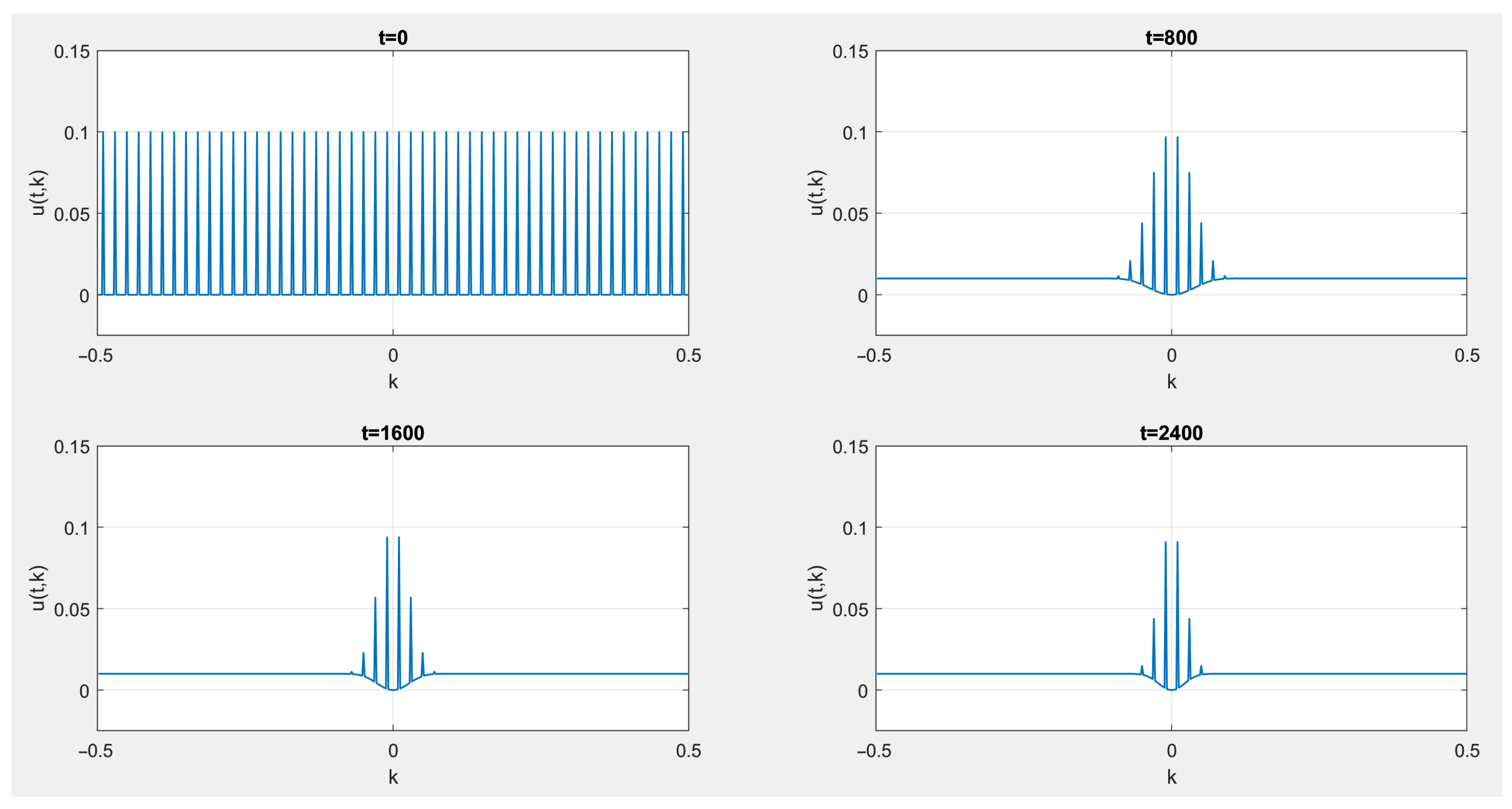
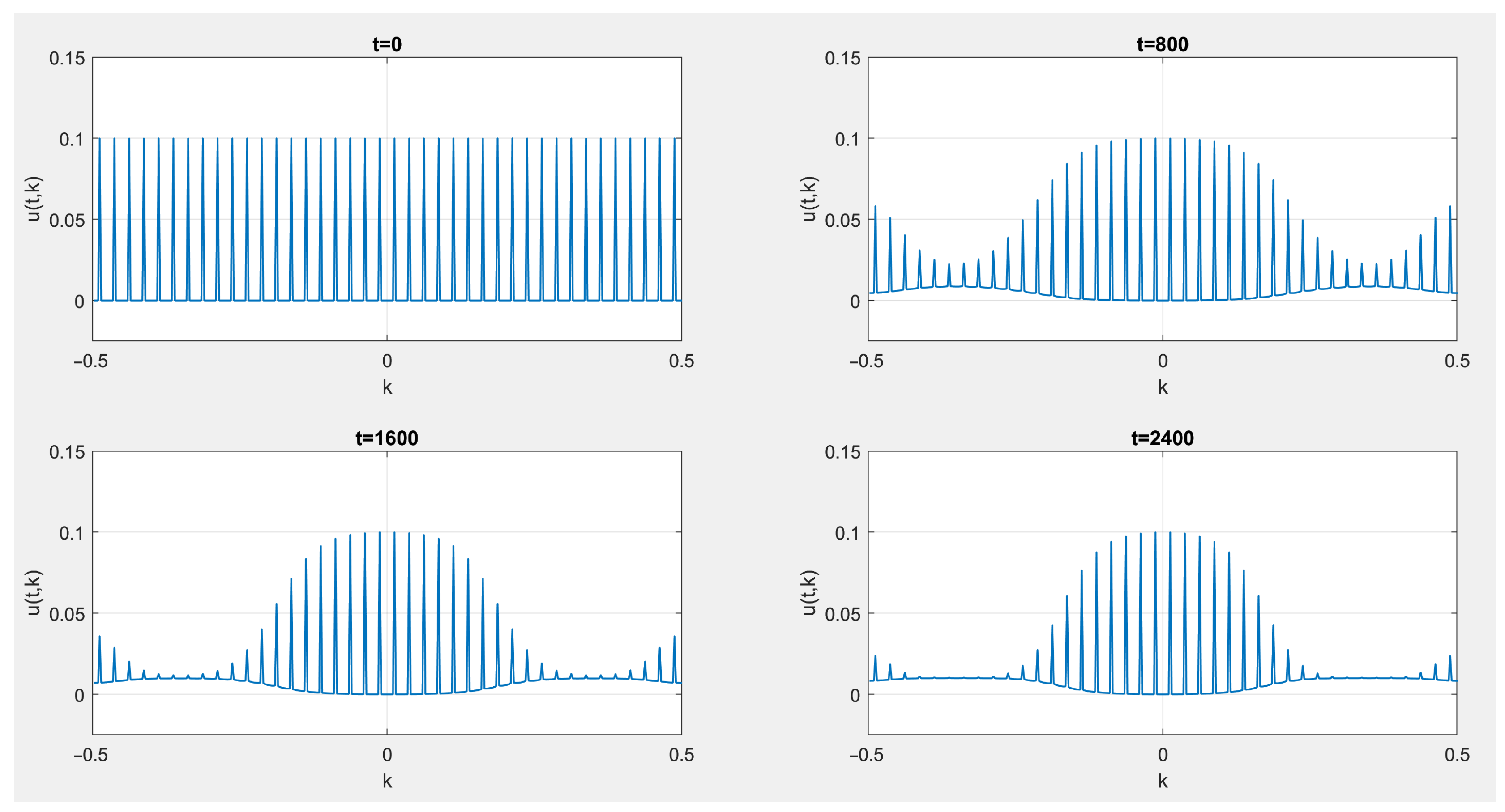
We impose the initial condition highly unevenly distributed over normal modes (see the graph for on Figure 5), and we solve (27) numerically. For the model with Gaussian noise, i.e., with collision kernel (10) we obtain the following picture of , at chosen time instants, seen on Figure 5.
Initially, the energy is set concentrated on modes −0.03, −0.01, 0.01, 0.03, 0.05… After 2400 time steps, we observe that energy is uniformly distributed over all modes outside a small vicinity of 0; however, the spikes closest to are still visible. This corresponds to the fact that long-wave energy is not susceptible to dissipation, which results in superdiffusive heat flow. Now, let us consider the scattering rates obtained from linear dynamics with Ornstein–Uhlenbeck perturbation, i.e., determined by the kernel (12). We made both models comparable by normalizing both kernels, i.e., by dividing each by . If the scattering rates are given by (12) with and being a positive constant functions (and therefore separated from zero), the plots of energy distribution are as seen on Figure 6.
The tendency of long waves to conserve energy has strengthened. However, as we indicated in the introductory chapters, the superdiffusion coefficient still emerges from such dynamics. The way to change the situation is to let when . Letting , , we observe a radical change in the picture of the evolution of the energy distribution with respect to normal mode, see Figure 7.
The tendency of long waves to conserve energy increased significantly, and interestingly, we also see that the modes related to short wavelengths—in neighborhood of 1/2 (−1/2)—became conservative. The picture of energy evolution when we admit indefinitely long time correlation is so different from the first two simulations for superdiffusion with the parameter equal to 3/2 that it may confirm the hypothesis about the assumption leading to the superdiffusion model with different from 3/2. The final confirmation should be made by mathematical considerations discussed in the next section.
4. Discussion and Future Work
The Ornstein–Uhlenbeck random field , in contrast to the Gaussian noise, has non-zero correlations over time and thus appears to be more natural for modeling a physical process which has some inertia. In [17], this Ornstein–Uhlenbeck process was defined as stationary Gaussian random field with postulated covariance function (16). The appropriate theorem guarantees its existence, see Theorem 8.2 in [30]. It has properties of a Markov process; however, to our knowledge, there is no transition probability function for it that meets the definition given in [35] p. 156. In the present work, we proceed a different path of construction of . We construct the function , which has a properties of transition probability (let us call it quasi-transition probability function) that allows constructing Markov processes whose stationary representative is the Ornstein–Uhlenbeck process introduced in [17]. The construction of the function was the most difficult task. The quasi-transition probability function allows for a different approach to the analysis of equations with such a disturbance. With this approach, we can think of weakening the assumptions on temporal correlations for such a process, which may be of great importance for the heat flow model. The collision kernel (12) depends on the time correlation of OU perturbation, and we would like to meet the condition (13). This can be fulfilled by making the function dependent on the scaling parameter , which tends to zero while approaching the macroscopic scale. Namely, we define the function , where is assumed to satisfy (13). While the parameter tends to zero, and we asymptotically approach the situation when time correlations are indefinitely long. The presented methodology is a very extensive task that goes beyond the scope of current project. Therefore, it will be further pursued in our subsequent research. Consequently, our objective is to derive a superdiffusive heat equation with an coefficient that differs from 3/2.
Author Contributions
Conceptualization, Z.A.Ł.; validation, Z.A.Ł. and Ł.S.; formal analysis, Ł.S.; writing—review and editing, Z.A.Ł. and Ł.S.; visualization, Ł.S. All authors have read and agreed to the published version of the manuscript.
Funding
This research was funded by Lublin University of Technology, grant numbers FN-17, FD-20/IT-3/011 and FD-20/IT-3/030. The APC was funded by Lublin University of Technology.
Data Availability Statement
Not applicable.
Conflicts of Interest
The authors declare no conflict of interest.
References
- Lepri, S.; Livi, R.; Politi, A. Heat conduction in chains of nonlinear oscillators. Phys. Rev. Lett. 1997, 78, 1896–1899. [Google Scholar] [CrossRef]
- Benenti, G.; Lepri, S.; Livi, R. Anomalous Heat Transport in Classical Many-Body Systems: Overview and Perspectives. Front. Phys. 2020, 8, 292. [Google Scholar] [CrossRef]
- Balandin, A.A. Thermal Properties of Graphene and Nanostructured Carbon Materials. Nat. Mater. 2011, 10, 569–581. [Google Scholar] [CrossRef] [PubMed]
- Chang, C.W. Experimental probing of non-fourier thermal conductors. In Thermal Transport in Low Dimensions: From Statistical Physics to Nanoscale Heat Transfer; Lepri, S., Ed.; Springer: Berlin/Heidelberg, Germany, 2016; pp. 305–338. [Google Scholar]
- Bernardin, C. Hydrodynamics for a System of Harmonic Oscillators Perturbed by a Conservative Noise. Stoch. Process. Appl. 2007, 117, 487–513. [Google Scholar] [CrossRef]
- Komorowski, T.; Olla, S. Ballistic and superdiffusive scales in macroscopic evolution of a chain of oscillators. Nonlinearity 2016, 29, 962–999. [Google Scholar] [CrossRef]
- Komorowski, T.; Olla, S. Diffusive propagation of energy in a non-acoustic chain. Arch. Ration. Mech. Anal. 2017, 223, 95–139. [Google Scholar] [CrossRef]
- Komorowski, T.; Olla, S. Kinetic limit for a chain of harmonic oscillators with a point Langevin thermostat. J. Funct. Anal. 2020, 279, 108764. [Google Scholar] [CrossRef]
- Lepri, S.; Livi, R.; Politi, A. On the anomalous thermal conductivity of one-dimensional lattices. Europhys. Lett. 1998, 43, 271–276. [Google Scholar] [CrossRef]
- Lepri, S.; Livi, R.; Politi, A. Thermal Conduction in Classical Low-Dimensional Lattices. Phys. Rep. 2003, 377, 1–80. [Google Scholar] [CrossRef]
- Lepri, S.; Livi, R.; Politi, A. Universality of Anomalous One-Dimensional Heat Conductivity. Phys. Rev. E 2003, 68, 067102. [Google Scholar] [CrossRef] [PubMed]
- Basile, G.; Bernardin, C.; Olla, S. Momentum Conserving Model with Anomalous Thermal Conductivity in Low Dimension. Phys. Rev. Lett. 2006, 96, 204303. [Google Scholar] [CrossRef] [PubMed]
- Basile, G.; Olla, S.; Spohn, H. Energy Transport in Stochastically Perturbed Lattice Dynamics. Arch. Ration. Mech. 2010, 195, 171–203. [Google Scholar] [CrossRef]
- Jara, M.; Komorowski, T.; Olla, S. Limit Theorems for Additive Functionals of a Markov Chain. Ann. Appl. Prob. 2009, 19, 2270–2300. [Google Scholar] [CrossRef]
- Basile, G.; Bovier, A. Convergence of a Kinetic Equation to a Fractional Diffusion Equation. Markov Proc. Relat. Fields 2010, 16, 15–44. [Google Scholar]
- Komorowski, T.; Stępień, Ł. Long Time, Large Scale Limit of the Wigner Transform for a System of Linear Oscillators in One Dimension. J. Stat. Phys. 2012, 148, 1–37. [Google Scholar] [CrossRef]
- Komorowski, T.; Stępień, Ł. Kinetic Limit for a Harmonic Chain with a Conservative Ornstein-Uhlenbeck Stochastic Perturbation. Kinet. Relat. Model. 2018, 11, 229–278. [Google Scholar] [CrossRef]
- Smith, A.N.; Norris, P.M. Microscale Heat Transfer. In Heat Transfer Handbook; Bejan, A., Kraus, A.D., Eds.; Wiley: Hoboken, NJ, USA, 2003; pp. 1309–1357. [Google Scholar]
- Basile, G.; Bernardin, C.; Olla, S. Thermal Conductivity for a Momentum Conservative Model. Comm. Math. Phys. 2009, 287, 67–98. [Google Scholar] [CrossRef]
- Bonetto, F.; Lebowitz, J.L.; Rey-Bellet, L. Fourier Law: A challenge to Theorists. In Mathematical Physics; Imperial College Press: London, UK, 2000; pp. 128–150. [Google Scholar]
- Balescu, R. Equilibrium and Nonequilibrium Statistical Mechanics; Wiley: Hoboken, NJ, USA, 1975. [Google Scholar]
- Stępień, Ł. Stochastic Processes and Heat Transport; Wydawnictwo Politechniki Lubelskiej: Lublin, Poland, 2021. [Google Scholar]
- Griffiths, D.J. Introduction to Quantum Mechanics; Prentice Hall: Hoboken, NJ, USA, 1995. [Google Scholar]
- Fermi, E.; Pasta, J.; Ulam, S. Studies of Non Linear Problems. In Collected Papers; University of Chicago Press: Chicago, IL, USA, 1965; Volume 2, pp. 978–988. [Google Scholar]
- Lukkarinen, J.; Spohn, H. Anomalous Energy Transport in the FPU-β Chain. Commun. Pure Appl. Math. 2008, LXI, 1753–1786. [Google Scholar] [CrossRef]
- Spohn, H. Nonlinear Fluctuating Hydrodynamics for Anharmonic Chains. J. Stat. Phys. 2014, 154, 1191–1227. [Google Scholar] [CrossRef]
- Da Prato, G. An Introduction to Infinite-Dimensional Analysis; Springer: Berlin/Heidelberg, Germany, 2006. [Google Scholar]
- Shigekawa, I. Stochastic Analysis; Translations of Mathematical Monographs; American Mathematical Society: Ann Arbor, MI, USA, 2004; Volume 224. [Google Scholar]
- Adler, R.J. Geometry of Random Fields; Wiley: Hoboken, NJ, USA, 1981. [Google Scholar]
- Janson, S. Gaussian Hilbert Spaces; Cambridge University Press: Cambridge, UK, 1997. [Google Scholar]
- Stroock, D.W. Abstract Wiener Space, Revisited. Commun. Stoch. Anal. 2008, 2, 145–151. [Google Scholar] [CrossRef]
- Kukush, A. Gaussian Measures in Hilbert Space, Construction and Properties; Wiley: Hoboken, NJ, USA, 2020. [Google Scholar]
- Edwards, R.E. Fourier Series, A Modern Introduction, 2nd ed.; Springer: Berlin/Heidelberg, Germany, 1979; Volume 1. [Google Scholar]
- Katznelson, Y. An Introduction to Harmonic Analysis; Cambridge University Press: Cambridge, UK, 2004. [Google Scholar]
- Ethier, S.N.; Kurtz, T.G. Markov Processes, Characterization and Convergence; Wiley: Hoboken, NJ, USA, 2009. [Google Scholar]
Figure 1.
The model of vibrational energy transport through a one-dimensional crystalline lattice—linear chain of atoms oscillating around their equilibrium positions. Bonds between neighboring atoms are drawn as springs ([18], p. 1317).
Figure 1.
The model of vibrational energy transport through a one-dimensional crystalline lattice—linear chain of atoms oscillating around their equilibrium positions. Bonds between neighboring atoms are drawn as springs ([18], p. 1317).
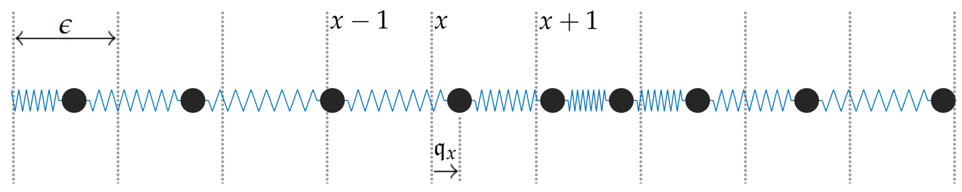
Figure 2.
Energy carriers—sinusoidal oscillations, —group velocity of mode k.
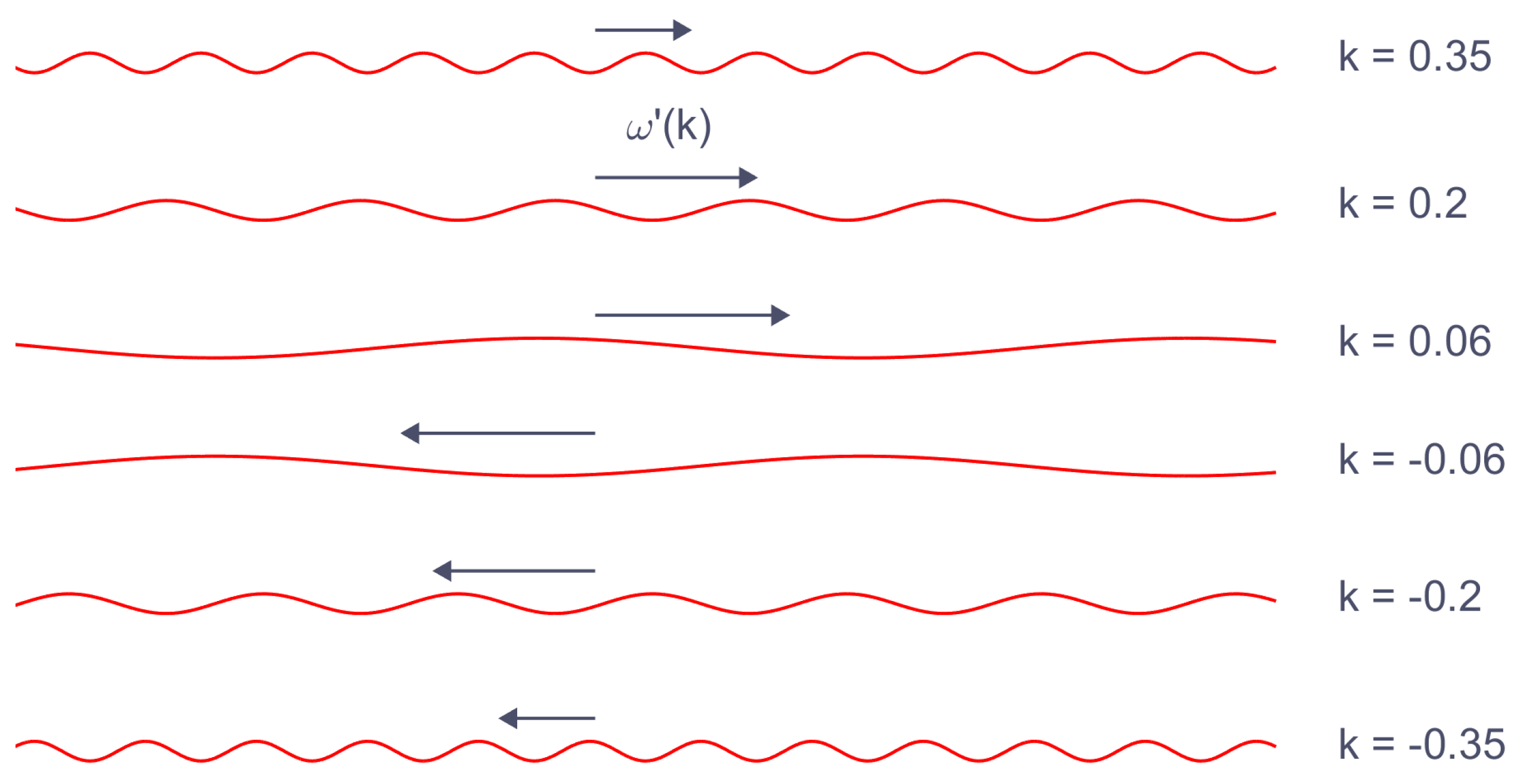
Figure 3.
A wave packet—superposition of normal modes—propagates through the medium with the group velocity, which is determined by the derivative of the dispersion relation.
Figure 3.
A wave packet—superposition of normal modes—propagates through the medium with the group velocity, which is determined by the derivative of the dispersion relation.

Figure 4.
Different scales of dynamics for a model of heat energy transport.

Figure 5.
Evolution of energy distribution on normal modes under the regime of linear Boltzmann equation related to Gaussian noise perturbation at the microscopic scale. The initial distribution does not depend on space variable x.
Figure 5.
Evolution of energy distribution on normal modes under the regime of linear Boltzmann equation related to Gaussian noise perturbation at the microscopic scale. The initial distribution does not depend on space variable x.
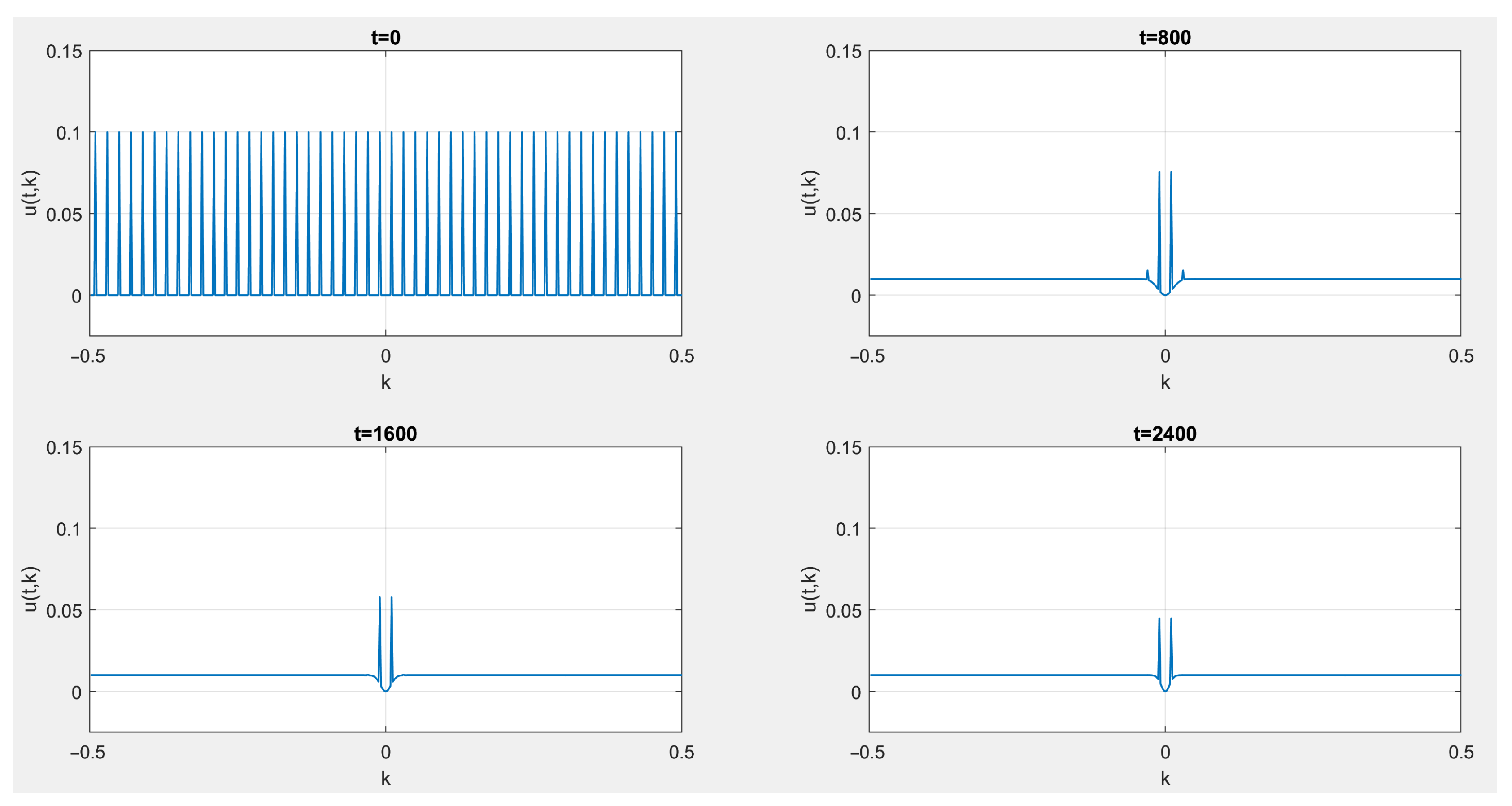
Figure 6.
Evolution of energy distribution on normal modes under the regime of linear Boltzmann equation related to Ornstein–Uhlenbeck perturbation at the microscopic scale, with and . The initial distribution does not depend on space variable x.
Figure 6.
Evolution of energy distribution on normal modes under the regime of linear Boltzmann equation related to Ornstein–Uhlenbeck perturbation at the microscopic scale, with and . The initial distribution does not depend on space variable x.

Figure 7.
Evolution of energy distribution on normal modes under the regime of linear Boltzmann equation related to Ornstein–Uhlenbeck perturbation at the microscopic scale, with and . The initial distribution does not depend on space variable x.
Figure 7.
Evolution of energy distribution on normal modes under the regime of linear Boltzmann equation related to Ornstein–Uhlenbeck perturbation at the microscopic scale, with and . The initial distribution does not depend on space variable x.
Disclaimer/Publisher’s Note: The statements, opinions and data contained in all publications are solely those of the individual author(s) and contributor(s) and not of MDPI and/or the editor(s). MDPI and/or the editor(s) disclaim responsibility for any injury to people or property resulting from any ideas, methods, instructions or products referred to in the content. |
© 2023 by the authors. Licensee MDPI, Basel, Switzerland. This article is an open access article distributed under the terms and conditions of the Creative Commons Attribution (CC BY) license (https://creativecommons.org/licenses/by/4.0/).
Share and Cite
MDPI and ACS Style
Stępień, Ł.; Łagodowski, Z.A. A Stochastic Model of Anomalously Fast Transport of Heat Energy in Crystalline Bodies. Energies 2023, 16, 7117. https://doi.org/10.3390/en16207117
AMA Style
Stępień Ł, Łagodowski ZA. A Stochastic Model of Anomalously Fast Transport of Heat Energy in Crystalline Bodies. Energies. 2023; 16(20):7117. https://doi.org/10.3390/en16207117
Chicago/Turabian StyleStępień, Łukasz, and Zbigniew A. Łagodowski. 2023. "A Stochastic Model of Anomalously Fast Transport of Heat Energy in Crystalline Bodies" Energies 16, no. 20: 7117. https://doi.org/10.3390/en16207117
Note that from the first issue of 2016, this journal uses article numbers instead of page numbers. See further details here.