Improved Delayed Detached Eddy Simulation of Combustion of Hydrogen Jets in a High-Speed Confined Hot Air Cross Flow

Abstract

The paper deals with the self-ignition and combustion of hydrogen jets in a high-speed transverse flow of hot vitiated air in a duct. The Improved Delayed Detached Eddy Simulation (IDDES) approach based on the Shear Stress Transport (SST) model is used, which in this paper is applied to a turbulent reacting flow with finite rate chemical reactions. An original Adaptive Implicit Scheme for unsteady simulations of turbulent flows with combustion, which was successfully used in IDDES simulation, is described. The simulation results are compared with the experimental database obtained at the LAERTE experimental workbench of the ONERA—The French Aerospace Laboratory. Comparison of IDDES with experimental results shows a strong sensitivity of the simulation results to the surface roughness and temperature of the duct walls. The results of IDDES modeling are in good agreement with experimental pressure distributions along the wall and with the results of videoregistration of the excited radical chemiluminescence.

1. Introduction

The capabilities of experimental studies of hot high-speed flows in ducts are very limited, and, in the field of numerical simulation, the level of accuracy and reliability of the results required for practice has not yet been achieved. In this regard, the task of further development, validation and tuning of numerical models is particularly relevant. However, such model development is very difficult without access to experimental data sets specifically designed for validation of mathematical models and computer codes based on them.

The amount of experimental data on combustion in high-speed free and confined flows in open sources is extremely limited. The classical experiments, often used for the assessment of physical and mathematical models, deal with the combustion in free jets and boundary layers [1,2,3,4,5,6]. Combustion in high-speed confined flows, i.e., in the ducts of different geometrical complexity (with pylons, steps, caverns, etc. used for fuel injection and combustion stabilization), was studied experimentally in numerous works (see, for example, [7,8,9,10,11,12,13,14]).

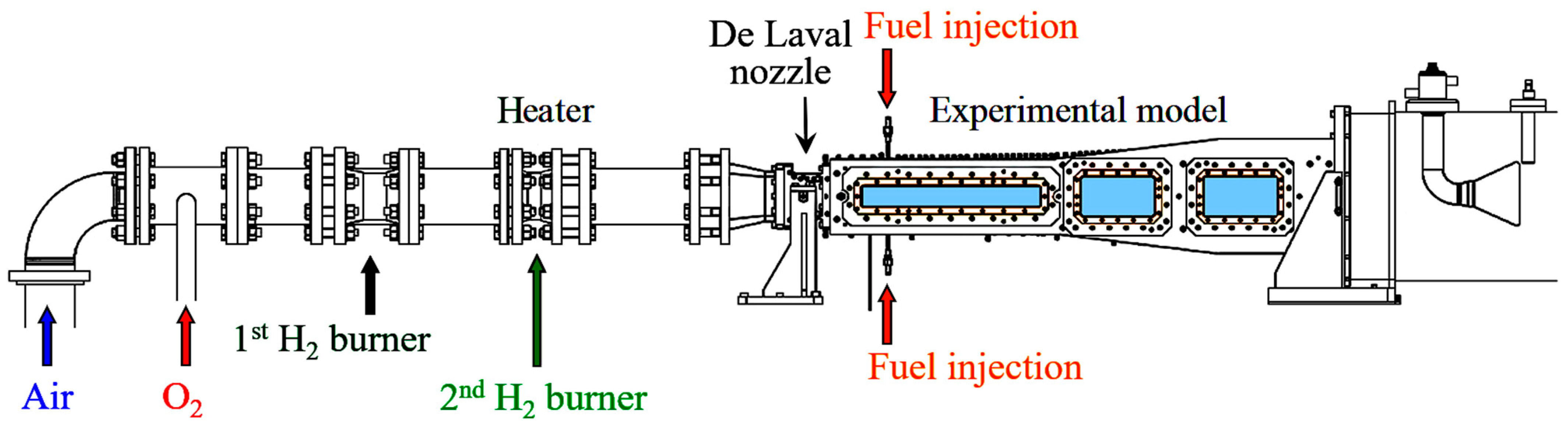
A recent experiment on high-speed combustion performed at ONERA, the French Aerospace Laboratory, at LAERTE test facility [15] was designed specially to create a database for assessment and validation of physical and mathematical models of high-speed reacting flows by means of numerical simulations. In this experiment, combustion of hydrogen jets in a high-speed hot air cross flow in a model duct of rectangular cross-section with a constant lateral width was explored. The geometry of the model duct was chosen in such a way that, with the flow parameters considered in the experiments at the entrance to the model duct ($M_{in}=2$, $T_{tot,in}=1400\dots 1700$ K, $\phi =0.15$), self-ignition of fuel in a high-speed flow was obtained and a stationary thermal choking of the duct did not occur. To achieve a high stagnation temperature of the flow, the air was preheated by a fire heater with hydrogen combustion and oxygen enrichment of combustion products. Vitiated “air” was formed in the heater, containing hydrogen combustion products–water vapor and radicals. This “air” was supplied under pressure to the Laval nozzle, accelerating the flow to Mach number $M\approx 2$. A model duct 1.192 m long with a side width of 0.04 m was installed at the outlet of the Laval nozzle (Figure 1). The half-height of the entrance section was 0.0177 m. Fuel (hydrogen) was blown perpendicular to the flow from the upper and lower walls. The model was equipped with optical windows located along the entire length of the duct, which made it possible to visualize the flow structure using high-speed Schlieren videography and to register the chemiluminescence of excited OH* radicals. The distributions of the average static pressure over time were measured, as well as the profiles of the stagnation temperature at the entrance to the model duct. The analysis of experimental data has shown the presence of a number of flow modes fundamentally different in the structure of the flow in the model [15].

The researchers at ONERA have performed a number of works on numerical modeling of these experiments, both within the framework of the Reynolds equations (RANS) [15,16,17] and on the basis of hybrid RANS/LES approaches combining RANS in the wall region with eddy-resolving simulation in the rest of the flow region [18,19]. The computational work has shown the complexity of modeling high-speed combustion in the duct, even in such a simplified experiment. Some results of the experiment could not be replicated in simulations.

At TsAGI, work on numerical modeling of ONERA experiments was started in 2019. For simulations, the in-house zFlare code [20] was used, developed at the Laboratory of physical and numerical simulation of flows with turbulence and combustion (TsAGI) [21]. The first results were published in the article [22].

In [22], RANS simulations of the flow in the heater and the nozzle are described, which provided the distribution of parameters at the entrance to the model duct. The preliminary RANS simulations of the flow in the model duct are also presented. It was found that reactions involving peroxides are important for the simulation of the flow in the heater and the nozzle, but have insignificant impact on the pressure distribution along the duct walls. At the same time, a strong influence of the wall temperature was found. The results of TsAGI simulations showed good agreement with ONERA simulations in a similar formulation [17]. However, both simulations differ greatly from the experimental data [15] in pressure distributions.

In the simulations of TsAGI, conducted in 2019 [22], as well as in similar simulations of ONERA [17], the duct walls were considered smooth. However, in the experiment, the walls were covered with a heat-protective coating of zirconium and yttrium oxides (YSZ, Yttria Stabilized Zirconia), and this led to the fact that the inner surface of the duct was rough. In experiments [15] it was found that the characteristic roughness height was about 65 μm. Taking into account the roughness in the ONERA simulations, also presented in [17], allowed a pressure distribution significantly closer to the experiment to be obtained.

The paper [23] presents the results obtained on this subject in TsAGI in 2020–2021. All these simulations were carried out taking into account the roughness of the duct walls.

In one experiment [15], longitudinal oscillations of the combustion zone and shock-wave structures located above the heat release zone in the inviscid core of the flow were observed. The experience of flow simulations in a model duct based on the Reynolds equations, described by Pelletier et al. [17], gave a stationary picture of the flow. In order to obtain longitudinal oscillations, it seems necessary to take into account non-stationary turbulent effects in the combustion zone. As the experience described in [18,19] shows, this can be achieved within the framework of a hybrid RANS/LES approach.

One study [23] describes the first attempt to perform simulations of the ONERA model using zFlare code on the basis of the SST-IDDES approach [24]. The significant influence of wall roughness was confirmed. However, the IDDES simulation predicted the flame shifted downstream compared with the experiment. This result was obtained both with the use of the wall function for rough walls [25] and with the no-slip boundary condition for rough walls, proposed in [26] and used in ONERA simulations [17].

That is why a series of studies was carried out in the RANS formulation, in which the influence of chemical kinetics, variable Prandtl number, roughness height, and heat exchange conditions on the duct walls was investigated. This series of simulations is also described in [23]. It transpires that the pressure distribution along the duct is most strongly influenced by the roughness height and by the temperature of the duct walls. However, there is an estimate of 65 µm for the roughness height, recommended in [17] based on experimental results. However, the temperature of the walls can be considered as an indefinite parameter in this problem. During one experiment [15], the attempt to determine the wall temperature failed, so the RANS simulations were performed with different values of the wall temperature T_W. The best agreement with the experimental pressure distribution was achieved at T_W = 1413 K [23].

The present article describes the mathematical formulation and the results of the main series of IDDES simulations. This series was performed with the use of the task parameters chosen in the above-mentioned RANS simulations. Calculations were carried out on the RFNC VNIIEF supercomputer [27], and 3000 CPU cores were used. The total amount of memory for the simulation was 830 GB. The simulation required 2.2 million core hours of CPU time. In comparison with preliminary IDDES simulations described in [23], the mesh with near-wall refinement was used, and a much longer interval of physical time (11 ms) was simulated. Longitudinal oscillations of flame were obtained. Comparison of the IDDES results with the experiment and with the RANS simulation [23], performed on the same mesh with the same parameters of the task, brings some light to the flow physics in the ONERA experimental model and also raises new questions, which should be analyzed in the future.

Section 2 describes a mathematical flow model used in simulations, and Section 3 presents an original numerical method that has been successfully used in IDDES simulations. Section 4 describes the organization of simulations and their main results. Section 5 is devoted to the analysis of the obtained physical flow pattern. Finally, Section 6 summarizes the results obtained and analyzes possible ways to improve the flow model.

2. Mathematical Model of the Flow

In this paper, SST-IDDES [24] is used as an eddy-resolving approach, which is applied to high-speed turbulent flow with finite-rate combustion. The chosen approach belongs to the DES family. DES is a hybrid approach that combines URANS at solid walls with LES in the rest of the flow region. Two modifications of DES based on the SST turbulence model were proposed in [24]: DDES, which is designed to simulate attached boundary layers over the entire thickness in the URANS mode, and IDDES, which allows the model to operate in the boundary layer either in the URANS mode over the entire thickness (if no perturbations are introduced into the solution), or in the LES mode in the outer part of the boundary layer, if the boundary layer in some section is perturbed by an external action. In this case, the basic system of equations can be represented as follows:

$$\frac{\partial u}{\partial t}+\frac{\partial f_j^{Eu}}{\partial x_j}+\frac{\partial f_j^{NS}}{\partial x_j}=s$$

(1)

$$u=\left[\begin{array}{c}\rho \\ \rho u_i\\ \rho E\\ \rho k\\ \rho \omega \\ \rho Y_l\end{array}\right]\hspace{0.17em},\hspace{0.17em}{f}_j^{Eu}=\left[\begin{array}{c}\rho u_j\\ \rho u_i{u}_j+p{\delta }_{ij}\\ (\rho E+p)u_j\\ \rho k{u}_j\\ \rho \omega u_j\\ \rho Y_l{u}_j\end{array}\right]\hspace{0.17em},\hspace{0.17em}{f}_j^{NS}=\left[\begin{array}{c}0\\ {\tau }_{ij}\\ {\tau }_{ij}{u}_i+{\Theta }_j+{\displaystyle {\sum }_l{J}_j(Y_l)h_l}\\ J_j(k)\\ J_j(\omega )\\ J_j(Y_l)\end{array}\right]\hspace{0.17em},\hspace{0.17em}s=\left[\begin{array}{c}0\\ 0\\ 0\\ S(k)\\ S(\omega )\\ S(Y_l)\end{array}\right]\hspace{0.17em}.$$

Here $u$ is a vector of conservative variables, $f_j^{Eu}$ is a flux of the $u$ vector in the Cartesian axis direction $x_j$, associated with convection (the gas movement as a continuous medium) and with pressure forces, $f_j^{NS}$ is a flux of the $u$ vector in the Cartesian axis direction $x_j$, associated with molecular diffusion and turbulent fluctuations, $s$ is a source term vector. In addition to the vector of conservative variables, the vector of primitive variables $p={\left[T,u_i,p,k,\omega ,Y_l\right]}^{\mathrm{T}}$ will also be used. Vectors $u$, $f_j$, $s$, $p$ have a dimension $7+N_{sp}$, where $N_{sp}$ is the total number of the mixture components. The gas is considered as a reacting mixture of gaseous components, each of which satisfies the Mendeleev–Clapeyron state equation.

The summation by repeated spatial indices (i, j or n) is assumed. All parameters are averaged (RANS) or filtered (LES) according to the Favre rules. Averaging/filtering signs are omitted, except where they are needed.

In the system (1), $E=u_n{u}_n/2+k+h-p/\rho$ is the total energy per unit mass of the gases mixture, where $h={\displaystyle {\sum }_l{Y}_l{h}_l}(T)$ is the mixture enthalpy that includes chemical energy. ${\tau }_{ij}=\frac{2}{3}\rho k{\delta }_{ij}-\left(\mu +{\mu }_{\mathrm{T}}\right)\left[\frac{\partial u_i}{\partial x_j}+\frac{\partial u_j}{\partial x_i}-\frac{2}{3}\frac{\partial u_n}{\partial x_n}{\delta }_{ij}\right]$ is the total (molecular and turbulent) flux of the i-th momentum component along the $x_j$ axis. ${\Theta }_j=-\left(\frac{\mu }{\mathrm{Pr}(h)}+\frac{{\mu }_{\mathrm{T}}}{{\mathrm{Pr}}_{\mathrm{T}}(h)}\right)c_p\frac{\partial T}{\partial x_j}$ is the total heat flux along the $x_j$ axis associated with temperature gradients (the molecular and turbulent Prandtl numbers are assumed to be equal to $\mathrm{Pr}(h)=0.72$, ${\mathrm{Pr}}_{\mathrm{T}}(h)=0.9$ by default). $J_j(k)=-\left(\frac{\mu }{\mathrm{Pr}(k)}+\frac{{\mu }_{\mathrm{T}}}{{\mathrm{Pr}}_{\mathrm{T}}(k)}\right)\frac{\partial k}{\partial x_j}$, $J_j(\omega )=-\left(\frac{\mu }{\mathrm{Pr}(\omega )}+\frac{{\mu }_{\mathrm{T}}}{{\mathrm{Pr}}_{\mathrm{T}}(\omega )}\right)\frac{\partial \omega }{\partial x_j}$ are the total fluxes along the $x_j$ axis of the turbulence parameters k and ω. $S(k)$ and $S(\omega )$ are the source terms in the equations for k and ω. $J_j(Y_l)=-\left(\frac{\mu }{\mathrm{Sc}}+\frac{{\mu }_{\mathrm{T}}}{{\mathrm{Sc}}_{\mathrm{T}}}\right)\frac{\partial Y_l}{\partial x_j}$ is the total flux of $Y_l$ along the $x_j$ axis ($\mathrm{Sc}=0.9$,${\mathrm{Sc}}_{\mathrm{T}}=1.0$).

The source term in the equation for $Y_l$ reads: $S(Y_l)=-m_l{\displaystyle {\sum }_r{\nu }_{lr}{\dot{\omega }}_r}$. In this paper, the effect of the turbulence on the average chemical reaction rates is not taken into account. LES simulations of high-speed confined reacting flow with the use of turbulence-combustion interaction (TCI) models requires significant additional work. This is a reason why the inclusion of the TCI model goes beyond the scope of the present study. In any way, study of the role of TCI on the flow structure assumes a preliminary simulation neglecting this effect.

The system (1) is closed by the state equation $p=\rho R_{0}T{\displaystyle {\sum }_l{Y}_l{m}_l^{-1}}$, the Sutherland formula for molecular viscosity $\mu =1.72\cdot {10}^{-5}{\left(\frac{T}{273}\right)}^{3/2}\frac{273+122}{T+122}$ [N∙m⁻²s⁻¹] and approximations of the $h_l(T)$ dependencies from the database [8]. The heat capacity of the mixture is calculated as $c_p={\displaystyle {\sum }_l{Y}_{l}d{h}_l/dT}$. The values of empirical coefficients (including $\mathrm{Pr}(k)$, ${\mathrm{Pr}}_{\mathrm{T}}(k)$, $\mathrm{Pr}(\omega )$ and ${\mathrm{Pr}}_{\mathrm{T}}(\omega )$)) and expressions for turbulent viscosity and source terms of the SST model are taken from [28].

In the SST turbulence model the source terms in the equation for k can be written in the form $\rho (P_k-\epsilon )$, where $P_k$ is the production of the turbulence kinetic energy, and $\epsilon$ is its dissipation rate: $\epsilon =\rho k^{3/2}/L$. The length scale is calculated by the formula $L=L_{\mathrm{RANS}}=\sqrt{k}/(C_{\mu }\omega )$, where $C_{\mu }=0.09$. As part of the DES approach, the length scale is replaced by a hybrid formula: $L=L_{\mathrm{DES}}={\tilde{f}}_d{L}_{\mathrm{RANS}}+\left(1-{\tilde{f}}_d\right)L_{\mathrm{LES}}$, where ${\tilde{f}}_d$ is the transition function equal to 1 in the RANS region and 0 in the LES region, and $L_{\mathrm{LES}}$ is the subgrid length scale. The expression for $L_{\mathrm{LES}}$ and for the ${\tilde{f}}_d$ function can be found in [24]. It should be noted that the values of the constants C_DES1 and $C_{DES2}$, which are used in determining the $L_{\mathrm{LES}}$ length scale, must be calibrated depending on the chosen numerical method [29]. In the current work, the value of C_DES1 = C_DES2 = 0.56 was employed, established in [30] using the simulations of the homogeneous isotropic turbulence decay. The shear layer adapted length scale, also described in [24], is used for accelerating the disturbance development in the mixing layers.

3. Numerical Method

All simulations are carried out on a fixed multi-block structured mesh with hexagonal cells. For spatial approximation, the 2nd order finite-volume method (which in the one-dimensional case has the 5th order) is used with one Gaussian point on each cell face. In the three-dimensional case, the extended stencil allows the reduction of the magnitude of the approximation error. The simulation is carried out by marching in time, when the initial flow field (at a time $t^0$) is known, and the solution for $t>t^0$ is obtained by successive transitions from a known time layer $t^n$, $n=0,\hspace{0.17em}1,\hspace{0.17em}2,\hspace{0.17em}\dots$, to the next layer, $t^{n+1}=t^n+{\tau }^n$.

Integrating the system (1) by the mesh cell volume and applying the Gauss–Ostrogradsky theorem, we represent it in the form

$$\frac{\partial U}{\partial t}+\frac{1}{V}{\displaystyle \sum _{g=1}^6{(F_j{\sigma }_j)}_g}=S,$$

(2)

where $F_j=F_j^{Eu}+F_j^{NS}$, ${\sigma }_g={\left({\sigma }_x,{\sigma }_y,{\sigma }_z\right)}^{\mathrm{T}}$ is the normal vector to the $g$-th cell face, the length of which is equal to the area of this face ($\left|{\sigma }_g\right|=A_g$), $U=\frac{1}{V}{\displaystyle \underset{V}{\int }udV}$ and $S=\frac{1}{V}{\displaystyle \underset{V}{\int }sdV}$ are the average over cell volume values of the conservative variable vector ${\left[\rho ,\rho u_i,\rho E,\rho k,\rho \omega ,\rho Y_l\right]}^T$ and of the source term vector, ${(F_j^{Eu})}_g=\frac{1}{A_g}{\displaystyle \underset{A_g}{\int }{f}_j^{Eu}dA}$ and ${(F_j^{NS})}_g=\frac{1}{A_g}{\displaystyle \underset{A_g}{\int }{f}_j^{NS}dA}$ are the flux vector ($f_j^{Eu}$ and $f_j^{NS}$) values, averaged over the $g$-th cell face area. A vector of primitive variables $P\left(U\right)={\left[T,u_i,p,k,\omega ,Y_l\right]}^T$ will also be used.

Convective fluxes are calculated using a hybrid scheme that combines an upwind approximation ${(F_j^{Eu})}_{\mathrm{upwind}}$ based on a five-point WENO reconstruction and a central difference approximation ${(F_j^{Eu})}_{\mathrm{central}}$ using a formula of the form

$$F_j^{Eu}=\sigma {(F_j^{Eu})}_{\mathrm{upwind}}+(1-\sigma ){(F_j^{Eu})}_{\mathrm{central}}.$$

The formulation of the weight function $\sigma$ proposed in [31] is used. This function depends on the local solution properties. It switches the scheme to an upwind mode in the RANS flow areas and in non-turbulent regions of almost undisturbed flow away from the study area. In the LES regions of the flow, the scheme approaches the central difference one, which makes its dissipativity significantly lower than that of a pure WENO scheme.

The $F_j^{NS}$ fluxes are calculated using formulas for $f_j^{NS}$ (see (1)), which contain gradients of flow parameters and also contain coefficients of molecular and turbulent diffusion that depend on local values of primitive variables. To approximate gradients in fluxes $F_j^{NS}$, a 2nd accuracy order modification of the central difference approximation is used [32]. The local values of the primitive variables vector $P$, used in $F_j^{NS}$, are calculated by linear interpolation between the neighboring cell centers.

In general, the fluxes are approximated on an unknown time layer $t=t^{*}$, i.e., time integration is carried out according to an implicit scheme. In the implicit part of the numerical method, the temporal linearization of fluxes is used. Fluxes through the face g on an unknown time layer are expressed in terms of fluxes on a known layer $n$:

$$\begin{array}{r}{\left(F_j(U^{*})\right)}_g\approx {\left(F_j(U^n)\right)}_g+\left(A_{0,g}^{Eu}(U^n)+A_{0,g}^{NS}(U^n)\right)\cdot \left(U^{*}-U^n\right)+\\ \left(A_g^{Eu}(U^n)+A_g^{NS}(U^n)\right)\cdot \left(U_g^{*}-U_g^n\right).\end{array}$$

(3)

Here $U_g$ is the conservative variables vector in the cell, which is located on the opposite side from the $g$-th face of the current cell. $A_{0,g}^{Eu}(U)$, $A_{0,g}^{NS}(U)$, $A_g^{Eu}(U)$ and $A_g^{NS}(U)$ are matrices that are calculated based on the flow parameters on a known layer n. The form of these matrices is given in [33].

The original Adaptive Implicit Scheme (AIS) is used for simulations. It is based on the following considerations:

• Since convective processes, as a rule, play a decisive role in the flow structure formation, it is important to describe them accurately. This means that in areas where non-stationary processes are of interest, the “convective” (classical) Courant number ${\mathrm{CFL}}^{Eu}\equiv \tau /{\tau }^{Eu}~0.5-1$ should be maintained. An explicit scheme can be used for this purpose. The implicit scheme should be activated only at the bottom of the boundary layer, where the sufficient time step value for describing non-stationary processes in the flow core will lead to ${\mathrm{CFL}}^{Eu}>1$. As a result, errors in the approximation of convective fluxes may increase there. However, the convective processes in the immediate vicinity of the wall are suppressed by viscosity and play a secondary role compared with diffusion. This statement is supported by the results of test simulations described below (see the end of this Section). In these tests, essentially viscous, quickly-changing unsteady flow was simulated using several approaches, and the AIS gave the same result as three other approaches, but appeared to be less time-consuming.
• Under the condition ${\mathrm{CFL}}^{Eu}~0.5-1$ in the flow core, diffusion processes are modeled in many areas with the explicit stability condition violation: ${\mathrm{CFL}}^{NS}\equiv \tau /{\tau }^{NS}>1$. Fortunately, there is evidence [34] that implicit schemes have an acceptably low error up to ${\mathrm{CFL}}^{NS}\approx 120$ for the diffusion equation. Therefore, it is sufficient to switch smoothly to the implicit approximation of diffusion fluxes when exceeding ${\mathrm{CFL}}^{NS}=1$ to ensure the scheme stability.

In AIS, to simulate reacting flows, the time step is performed using a two-stage Runge–Kutta (RK) procedure:

$$\begin{array}{l}{U}^{\left(1\right)}=U^n+\frac{1}{2}{\tau }^n\left[-\frac{1}{V}{\displaystyle \sum _{g=1}^6{\left(F_j(U^n){\sigma }_j\right)}_g}+S_1\right]+\\ w_{Eu}\frac{1}{2}{\tau }^n\cdot \left[A_{0,g}^{Eu}(U^n)\cdot \left(U^{(1)}-U^n\right)+A_g^{Eu}(U^n)\cdot \left(U_g^{(1)}-U_g^n\right)\right]+\\ w_{NS}\frac{1}{2}{\tau }^n\cdot \left[A_{0,g}^{NS}(U^n)\cdot \left(U^{(1)}-U^n\right)+A_g^{NS}(U^n)\cdot \left(U_g^{(1)}-U_g^n\right)\right],\\ U^{n+1}=U^{\left(2\right)}=U^n+{\tau }^n\left[-\frac{1}{V}{\displaystyle \sum _{g=1}^6{\left(F_j(U^{(1)}){\sigma }_j\right)}_g}+S_2\right]+\\ w_{Eu}{\tau }^n\cdot \left[A_{0,g}^{Eu}(U^{(1)})\cdot \left(U^{n+1}-U^{(1)}\right)+A_g^{Eu}(U^{(1)})\cdot \left(U_g^{n+1}-U_g^{(1)}\right)\right]+\\ w_{NS}{\tau }^n\cdot \left[A_{0,g}^{NS}(U^{(1)})\cdot \left(U^{n+1}-U^{(1)}\right)+A_g^{NS}(U^{(1)})\cdot \left(U_g^{n+1}-U_g^{(1)}\right)\right].\hspace{1em}\hspace{1em}\hspace{1em}\hspace{1em}\hspace{1em}\hspace{1em}\end{array}$$

(4)

In formula (4), the indices in parentheses indicate the stage number of the RK procedure, $U$ is the vector of conservative variables, $F_j(U^{\left(m\right)})$ are the fluxes calculated in the way described above by the known flow field obtained at the m-th stage of the RK procedure, and $S_{m+1}$ is the source terms approximation of this subsystem at the current (m + 1)-th stage. The implicit increments of the convective and diffusion fluxes with weights $w_{Eu}(CF{L}^{Eu})$, $w_{NS}(CF{L}^{NS},CF{L}^{Eu},w_{Eu})$, respectively, are also included in (4). The formulas for the weights are given below.

We divide the equations system (2) into three subsystems:

(1)

the basic (gas-dynamic) subsystem associated with the equations of mass, momentum and energy (the first five equations of the system);

(2)

the turbulent subsystem associated with the equations of the turbulence model (the following two equations);

(3)

the chemical subsystem associated with the equations for the reacting mixture components (the last N_sp equations).

Respectively, various terms of the system (2) can be represented as follows:

$$\begin{array}{l}U=\left[\begin{array}{c}{U}_{base}\\ U_{turb}\\ U_{chem}\end{array}\right]\hspace{0.17em},\hspace{1em}{F}_j=F_j^{Eu}+F_j^{NS}=\left[\begin{array}{c}{(F_j)}_{base}^{Eu}\\ {(F_j)}_{turb}^{Eu}\\ {(F_j)}_{chem}^{Eu}\end{array}\right]+\left[\begin{array}{c}{(F_j)}_{base}^{NS}\\ {(F_j)}_{turb}^{NS}\\ {(F_j)}_{chem}^{NS}\end{array}\right]\hspace{0.17em},\\ S=\left[\begin{array}{c}0\\ S_{turb}\\ S_{chem}\end{array}\right]=S_T+S_C,\hspace{1em}{S}_T=\left[\begin{array}{c}0\\ S_{turb}\\ 0\end{array}\right]\hspace{0.17em},\hspace{1em}{S}_C=\left[\begin{array}{c}0\\ 0\\ S_{chem}\end{array}\right]\hspace{0.17em}.\end{array}$$

(5)

For the basic subsystem, $S=0$.

A special interpretation of the source terms is used for the turbulent subsystem. Experience shows that the Jacobi matrix of the SST turbulence model source terms, $\partial S_{turb}/\partial U_{turb}$, is diagonally predominant. Of its two non-diagonal terms, one is zero and the other is much smaller in absolute value than the diagonal terms. Respectively, at the (m + 1)-th stage of the RK procedure, a linearized dependence $S_{turb}(U_{turb})$ can be approximately represented as

$$\begin{array}{l}S(k)\approx S{(k)}^{(m)}+{\lambda }_1\cdot \left(\rho k-{\rho }^{(m)}{k}^{(m)}\right),\\ S(\omega )\approx S{(\omega )}^{(m)}+{\lambda }_2\cdot \left(\rho \omega -{\rho }^{(m)}{\omega }^{(m)}\right),\end{array}$$

(6)

where ${\lambda }_1=\partial S(k)/\partial (\rho k)$, ${\lambda }_2=\partial S(\omega )/\partial (\rho \omega )$. A simple stability analysis of the source term approximations (see, for example, [32,34]) shows that, when solving an equation of the form $\frac{dp}{dt}=S_0+\lambda (p-p_0)$, $S_0=const$, $\lambda =const$, an explicit approximation $\frac{p^{n+1}-p^n}{\tau }=S_0+\lambda (p^n-p_0)$ at any time step gives a correct solution (positive and growing) if $\lambda \ge 0$, and for $\lambda <0$ it is stable only under the condition $\tau \le 1/\hspace{0.17em}\left|\lambda \right|$. On the contrary, an implicit approximation $\frac{p^{n+1}-p^n}{\tau }=S_0+\lambda (p^{n+1}-p_0)=\left[S_0+\lambda (p^n-p_0)\right]+\lambda (p^{n+1}-p^n)$ at any time step gives a correct solution (positive and decreasing) if $\lambda \le 0$, and for $\lambda >0$ it is stable only under the condition $\tau \le 1/\hspace{0.17em}\lambda$. We introduce a conditional “Courant number” (stability coefficient) for the source terms: $CF{L}^{source}=\tau /{\tau }^{source}(\lambda )$, where $\tau$ is the current time step value and ${\tau }^{source}(\lambda )={\left(-\min \left(\lambda ,{10}^{-20}\right)\right)}^{-1}$ is the time step limit for explicit approximation. It can be verified that a weighted combination of explicit and implicit approximations $\frac{p^{n+1}-p^n}{\tau }=\left[S_0+\lambda (p^n-p_0)\right]+w\cdot \lambda (p^{n+1}-p^n)$ gives the correct solution at any sign of $\lambda$ and at any time step, if the weight w is chosen to be equal

$$w_{source}\left(CF{L}^{source}\right)=\max \left(0,\frac{2CF{L}^{source}-1}{2CF{L}^{source}}\right).$$

(7)

Therefore, the following linear locally implicit approximation is used for the source terms of the turbulent subsystem:

$$S_{m+1}=\left[\begin{array}{c}S{(k)}^{(m)}+w_{source}\left(CF{L}_1^{source}\right)\cdot {\lambda }_1\cdot \left({\rho }^{(m+1)}{k}^{(m+1)}-{\rho }^{(m)}{k}^{(m)}\right)\\ S{(\omega )}^{(m)}+w_{source}\left(CF{L}_2^{source}\right)\cdot {\lambda }_2\cdot \left({\rho }^{(m+1)}{\omega }^{(m+1)}-{\rho }^{(m)}{\omega }^{(m)}\right)\hspace{0.17em}\end{array}\right],$$

(8)

where $CF{L}_k^{source}=\tau /{\tau }^{source}({\lambda }_k)$.

In the equations of the chemical subsystem, the source terms are interpreted differently. These terms contain highly nonlinear functions (reaction rates) that lead to a stiffness of the chemical subsystem [32]. Based on the experience described in [34], a nonlinear locally implicit approximation of the 2nd accuracy order in time is used for $S_{chem}$. To obtain this approximation, the first stage of the RK procedure is performed according to the formula

$$\begin{array}{l}{U}^{\left(1\right)}=U^n+\frac{1}{2}\tau \cdot \left[-\frac{1}{V}{\displaystyle \sum _{g=1}^6{\left(F_j(U^n){\sigma }_j\right)}_g}+S_T+S_C\left(U^{(1)}\right)\right]+\\ w_{Eu}\frac{1}{2}\tau \cdot \left[A_{0,g}^{Eu}(U^n)\cdot \left(U^{(1)}-U^n\right)+A_g^{Eu}(U^n)\cdot \left(U_g^{(1)}-U_g^n\right)\right]+,\\ w_{NS}\frac{1}{2}\tau \cdot \left[A_{0,g}^{NS}(U^n)\cdot \left(U^{(1)}-U^n\right)+A_g^{NS}(U^n)\cdot \left(U_g^{(1)}-U_g^n\right)\right]\hspace{0.17em}.\end{array}$$

(9)

In (9), $S_T$ is calculated by the formula (6) with m = 0. The value $S_C$ corresponds to the time moment $t=t^n+{\tau }^n/2$. After solving this system, the resulting value of the source term is stored and used unchanged at the second stage of the RK procedure (4): $S_2=S_1=S_C\left(U^{(1)}\right)$.

When performing step (9), the $\tau$ parameter is initially set to $\tau ={\tau }^n$. In the cases of the Newton’s iterations divergence or an unphysical solution, the procedure of locally fractional steps [32] is performed: the time step is divided by two, and two equal steps (9) are taken with $\tau ={\tau }^n/2$ without recalculation of fluxes. If this does not help, the time step is further divided, and four steps (9) are taken with $\tau ={\tau }^n/4$, etc. When it is possible to perform this procedure without a divergence of the Newton’s method and without the appearance of non-physical values, the full time step ${\tau }^n$ is repeated using the RK procedure (4). In this case, at all RK steps, the same value $S_C$ is used that is equal to the sum of the chemical sources values obtained at all locally fractional steps.

In AIS, in the areas where the explicit scheme is unstable at a given time step, implicit increments of convective and diffusion fluxes with the weights $w_{Eu}(CF{L}^{Eu})$, $w_{NS}(CF{L}^{NS},CF{L}^{Eu},w_{Eu})$, respectively, are added to the explicit scheme (see (4)). Adding these terms leads to the fact that, in the equation system (4), an unknown value $U^{(m+1)}$ in this cell is associated with unknown values in neighboring cells. Such a system is solved using the Gauss–Seidel block method [35].

The weights $w_{Eu}$ and $w_{NS}$ are determined using the following considerations. If we write down a one-step analog of the scheme (4) for the linear scalar advection equation $\frac{\partial u}{\partial t}+a\frac{\partial u}{\partial x}=0$, then the spectral stability analysis leads to the requirement $w_{Eu}\ge \frac{CF{L}^{Eu}-1}{2CF{L}^{Eu}}$. If we write down such a one-step scheme for the model advection–diffusion equation $\frac{\partial u}{\partial t}+a\frac{\partial u}{\partial x}=D\frac{{\partial }^{2}u}{\partial x^2}$, then the scheme will be stable under the condition $w_{NS}\ge \frac{CF{L}^{NS}-1+CF{L}^{Eu}\cdot (1-2w_{Eu})}{2CF{L}^{NS}}$. Based on these conditions, the weights of implicit increments in AIS for a nonlinear system of equations (2) are calculated using formulae that provide a transition to an explicit scheme under the conditions $CF{L}^{Eu}\le 1$, $CF{L}^{Eu}+CF{L}^{NS}\le 1$, and in other cases include some safety margin (overestimate the implicit scheme weight):

$$w_{Eu}=\max \left\{0,\frac{CF{L}^{Eu}-1}{CF{L}^{Eu}}\right\},\hspace{0.17em}\hspace{0.17em}{w}_{NS}=\max \left\{0,\frac{CF{L}^{NS}-1+\max \left(0,CF{L}^{Eu}\cdot (1-2w_{Eu})\right)}{CF{L}^{NS}}\right\}.$$

(10)

Thus, at a user-defined time step $\tau$, an explicit scheme with a multistep RK procedure is used in the cells where it is stable. In the remaining cells (usually these are cells in the near-wall regions of the boundary layers, where the flow becomes quasi-stationary, quickly rearranging under the action of non-stationary processes in the rest of the flow), a smooth transition to an implicit scheme of the 1st accuracy order based on linearization (3) is performed.

The authors of this paper compared the quality and efficiency of AIS with other methods of modeling unsteady flows. For this purpose, the problem with non-stationary combustion in the duct described in [36] was solved. Combustion simulations were carried out using the no-slip condition on the duct walls; the ratio of the mesh cell sizes was about 400. In addition, two explicit methods for simulating unsteady flows were considered—the global time stepping method and the fractional time stepping method [32], as well as the currently most popular implicit dual time stepping method. All four methods gave the same quality of the numerical solution. At the same time, the simulation according to the implicit scheme with a dual time stepping required 43 times less time than the simulation with a global time stepping, and the explicit scheme with a fractional time stepping gave an acceleration of 31 times, and AIS 85 times.

It should be noted that the efficiency ratio of the schemes decreases when the cell size difference decreases. On meshes with a 10–100 cell size ratio, an explicit scheme with a fractional time stepping usually works well (using wall functions) provided that the simulation can be parallelized effectively; AIS is comparable in cost, but is parallelized much easier. As for quasi-uniform grids, it is natural to choose the most reliable procedure—an explicit scheme with a global time stepping.

4. IDDES-Simulation of the Flow with Combustion in the ONERA Model

The mathematical model of the flow described above and the numerical method were applied to the simulation of the flow with combustion in the experimental model ONERA. The flow mode corresponding to “Case B” from [17] was considered. The geometry of the computational domain is shown in Figure 2. As in [17], only the lower half of the ONERA experimental model was considered in the simulations, since the flow in the experiment under the selected conditions can be considered symmetrical.

Initially, the RANS method was used to simulate the flow in the heater of the ONERA LAERTE aerodynamic stand. The heater simulation technology is described in [22]. The stagnation parameters on the axis of symmetry of the heater were assumed to be equal to p_tot = 4.07 bar and T_tot = 1705 K, and the temperature of the heater walls was set to 1490 K, in accordance with the data [15]. The combustion of a hydrogen–air mixture enriched with oxygen was simulated in the heater so that after the combustion the mass fraction of oxygen was close to the oxygen content in the air. Simulations were carried out taking into account HO₂ and H₂O₂ peroxides, because, according to the results from [22], this leads to a better prediction of the radical formation at the entrance to the duct of the experimental model. The distribution of parameters at the entrance to the experimental model obtained in the simulations of the heater was used as an inlet boundary condition for the IDDES simulation of the flow with combustion in the duct of the ONERA experimental model.

Fuel (hydrogen) was injected perpendicular to the flow through a hole with a diameter of 2 mm in the wall, on the vertical plane of symmetry of the duct, in the section x = 0.2 m (the injection site is shown by an arrow in Figure 2). The fuel consumption and the vitiated air entering the duct corresponded to the excess fuel ratio $\phi =0.153$. In accordance with the conclusions made in [22,23], the Jachimowski kinetics [37] without peroxides with seven reactions for seven components (H₂, O₂, H, O, OH, H₂O, N₂) were used to simulate the flow in the experimental model. Reactions and coefficients of this kinetic scheme are listed in

Table 1. Coefficients of forward reaction constants ¹ for the used kinetic scheme.

No.	Reaction	A	n	E
1	H2 + O2 = OH + OH	1.70 × 1013	0	48000
2	H + O2 = OH + O	2.60 × 1014	0	16800
3	OH + H2 = H2O + H	2.20 × 1013	0	5150
4	O + H2 = OH + H	1.80 × 1010	1	8900
5	OH + OH = H2O + O	6.30 × 1013	0	1090
6	H + H + M = H2 + M	6.40 × 1017	−1	0
7	H + OH + M=H2O + M	2.20 × 1022	−2	0

¹ “Constants” of the reaction rates are described by formula: k = ATⁿ exp(−E/R₀T). Measurement units are seconds, moles, cubic centimeters, calories and Kelvin degrees. For reactions 6, 7 the third-body efficiencies are the following: 2.5 for M = H₂, 16.0 for M = H₂O and 1.0 for all other M.

. Modifications of coefficients and third-body efficiencies (in comparison with [37]) are based on the paper [38].

The resolved turbulence was generated naturally as a result of the Kelvin–Helmholtz instability development in the mixing layer formed by the injected jet. Thus, upstream from the injection section the flow was modeled in the RANS mode.

The mesh used in the simulations was uniform in the LES region in the flow core, with almost cubic cells with edge length close to $1.5\cdot {10}^{-4}$ m. However, in the near-wall layer with a thickness of about 1.5 mm, this mesh was condensed to the wall (about 30 cells across the boundary layer). The total number of grid points was close to 92 million (2100 in the longitudinal, 140 in the transverse and 312 in the lateral direction, respectively). The height of the first near-wall cell was equal to $2\cdot {10}^{-5}$ m ($y^{+}~1$). Preliminary simulations of the flow around the flat plate with rough surface (with parameters taken from the entrance to the ONERA model) have shown that the mesh refinement does not change the boundary layer description. The scale-resolving region spans 0.18 m ≤ x ≤ 0.8 m in the longitudinal direction. There were 15 cells located across the injector opening. Within the scale-resolving region, the mesh was comparable to one used in DDES simulations by ONERA [19]. However, ONERA simulations used unstructured non-uniform mesh with adaptation to zones of high vorticity. To the contrary, TsAGI IDDES simulation was performed on structured, nearly uniform mesh (except the near-wall layers). It was less dense in the hydrogen jet mixing zone, but in the jet wake the resolution was higher than in ONERA simulations.

The no-slip boundary condition, taking into account the roughness of the walls, was imposed on the side and bottom walls. The roughness model based on study [26] was used. The characteristic roughness value was chosen to be 65 μm (in accordance with ONERA recommendations [17]). Based on the RANS simulations described in [23], the wall temperature was chosen to be 1413 K.

A boundary condition for supersonic outflow was imposed on the right boundary, and a symmetry condition was imposed on the upper boundary (according to ONERA experiments, the flow in the duct in this mode is almost symmetrical on average).

The final state of the preliminary IDDES simulation with the wall temperature T_W = 716 K was chosen as the initial field. This value of the wall temperature was used in ONERA simulations [17]. In TsAGI simulation with this wall temperature, combustion developed too far downstream from experimental location; the corresponding pressure distribution is shown in Figure 3 as a blue dotted curve).

Therefore, at the beginning of the simulation, the flow structure was rearranged, after which the flow entered a quasi-stationary mode. The typical time required for an inviscid flow to pass through the duct is about 1 ms. Figure 4 shows the dependence of the integral coefficient of the longitudinal wall friction force upon the physical time obtained in the IDDES simulation. The rearrangement of the flow structure took about 3 ms, after which two apparent “periods” of 3.5 ms each can be distinguished. By the end of the simulation, the full establishment of the stationary-on-the-average flow had not yet been achieved.

Figure 5 shows the time variation of the Mach number field in the vertical symmetry plane of the duct. It can be seen that at a time of 0.01 ms (shortly after the start of the simulation) in the vicinity of the plane of symmetry, the flow is supersonic everywhere. However, due to the increase in T_W, the growth of subsonic flow zones begins at the duct wall. In the next frame (0.5 ms), the flow core is almost completely displaced by the boundary layer. Disturbances propagate upstream along the duct. Then (1 ms) a shock wave is formed, moving upstream and causing the separation of the boundary layer. By the time of 2.5 ms, the separation zone is fixed in the wake of the injected jet and interacts with the gas-dynamic structure generated by the hydrogen jet. As a result of this interaction, locally favorable conditions for combustion arise. Large-scale movements of the boundary layer boundary lead to the fact that strong shock waves periodically arise in the core of the flow, forming local subsonic flow regions. Figure 5 also shows the moments close to the ends of the first and second apparent “periods” (see Figure 4), 6.5 ms and 9.5 ms.

It can be seen that, during the first apparent “period” (between moments d and e), there is a significant rearrangement of the shock-wave structure of the flow in the fuel injection area. At moment d (2.5 ms), a three-dimensional shock wave caused by the duct choking is located at $x\approx 0.215$ m. In the area of its intersection with the horizontal symmetry plane of the duct, a small region of subsonic flow is visible. By the end of the first “period” (6.5 ms) it shifts forward and stops upstream from the injected hydrogen jet. Due to the back pressure created by this shock wave, the separation upstream from the fuel jet increases in length and height. Due to the three-dimensional shape of the shock wave, the subsonic flow region near the symmetry plane of the duct in the jet vicinity disappears. During the second apparent “period”, the shock-wave structure in the vicinity of the injection almost does not change. Another subsonic region in the core of the flow continues to change shape and fluctuate between the coordinates 0.238 m and 0.242 m, sometimes increasing in size, sometimes decreasing (cf. moments d and f). Note that in RANS simulations by ONERA [17] the subsonic region turns out to be located in the flow core near the section of 0.236 m and occupies about 1 mm in each lateral direction from the symmetry plane.

5. Analysis of the Physical Flow Pattern

Here we compare the instantaneous flow field reached at the end of the IDDES simulation (11.13 ms) with the ONERA experiment and with the final (fully steady) state of RANS simulation of TsAGI with the same flow parameters published elsewhere [23].

The pressure distributions corresponding to these data sets are shown in Figure 3 (experiment—markers, RANS-simulation—red curve, IDDES-simulation—solid blue curve). It can be seen that in the eddy-resolving simulation, a larger pressure peak is obtained; it is shifted upstream relative to the solution obtained using the RANS simulation and relative to experimental data.

It is also worth noting that, in addition to the main peak, the pressure distribution is overestimated in the range from 0.3 m to 0.7 m in comparison with the experiment.

Figure 6 shows the experimental video recording of the excited OH radical chemiluminescence (showing the position of the main heat release region) superimposed on the shadow flow pattern.

Figure 7 compares the fields of Mach number, temperature and OH mass fraction in the vertical symmetry plane of the duct, obtained in the IDDES and RANS simulations of TsAGI.

There is no local choking in the RANS simulation of TsAGI (unlike the RANS simulation by ONERA [17]). The gas-dynamic structure of the shocks turns out to be significantly less intense than in the IDDES simulation. Therefore, in the RANS simulation, the separation zone is shifted downstream, which is closer to the experimental flow pattern.

In the fields of temperature and of OH mass fraction, it can be seen that, in IDDES and RANS simulations, both parameters increase near the hot wall in the wake of the injected jet. Then the heat release zone (which is characterized by large values of the OH mass fraction) shifts to the upper boundary of the boundary layer—to the area of the shock-wave interaction with the boundary layer.

Figure 8 demonstrates fields of the fuel excess ratio $\phi$, corresponding to Figure 7. This parameter was calculated employing the local mass ratio of unburnt fuel and air that lead to the local composition of reacting mixture. It was obtained using the local mass fraction of inert species—nitrogen. Taking into account that the composition of vitiated air at the duct entrance may be described approximately as ${\mathrm{O}}_2\hspace{0.17em}:\hspace{0.17em}{\mathrm{H}}_2\mathrm{O}\hspace{0.17em}:\hspace{0.17em}{\mathrm{N}}_2=0.248:0.167:0.585$, one may obtain the following formula for the fuel excess ratio:

$$\phi =\frac{8z}{0.248(1-z)},\hspace{1em}z=1-\frac{Y({\mathrm{N}}_2)}{0.585}$$

where z is the mixture fraction equal to 1 in pure fuel and 0 in pure air.

It is interesting that in the IDDES simulation the large part of the near wake past the hydrogen jet is filled by air, while in the RANS simulation the fuel penetrates into this area and participates in reactions. It may be explained by incorrect description of turbulent diffusion in the SST turbulence model used in the RANS simulation. This effect can explain why in the RANS simulation the combustion proceeds not only in the mixing layers of hydrogen jet but also in the near-wall layer.

Figure 9 shows a typical instantaneous field of the Mach number in the vertical symmetry plane of the duct. The superimposed arrows also depict instantaneous streamlines that start in the recirculation zones and come into the middle of the duct downstream. Thus, we can conclude that these zones are not closed. At the bottom left in Figure 9, one may see the injected hydrogen jet producing the recirculation zones both upstream and downstream from the injection (directly at the wall), as well as a shock wave (in the flow core), which in turn interacts with the boundary layer (slightly downstream). It is in the area of the shock wave interaction with the boundary layer where the chemical reaction is initiated. Thick black lines highlight the areas of increased OH mass fraction, showing the heat release zones. As a result of combustion near the wall, the boundary layer thickens and the flow core narrows till the local choking (in this figure at x = 0.238 m). A shock wave emerges. The gas that has passed through the heat release zone in the wake of the jet moves from the wall to the center of the duct, blends with the fresh combustible mixture in the flow core, heats it and adds radicals from the combustion zone to it. The interaction of this mixture with the emerged shock wave leads to formation of the main region of self-ignition.

The subsonic region that occurs during the choking is non-stationary. The shock-wave structure containing a normal shock wave oscillates along the longitudinal axis together with the combustion zone.

As can be seen from Figure 6, in the experiment, the main ignition region also occurs as a result of the shock-wave interaction with the boundary layer. At the same time, the combustion itself has an effect upstream due to the occurrence of local partial choking. The shock-wave structure in the experiment also fluctuates together with the separation region and with the combustion zone.

It is also worth noting that in the IDDES simulation the normal shock turns periodically into the intersection of oblique shocks, and the choking disappears. The extreme positions of local choking in the first “period” were 0.254 m and 0.236 m; qualitatively similar fields can be seen in Figure 5 at 6.5 and 9.5 ms, respectively. The duration of time, when the local choking was present in the first apparent “period”, was 3.2 ms (total duration of the “period” was 3.5 ms). In the second apparent “period” the subsonic regions were present all the time, although their vertical size varied from 2 mm to a complete overlap of the duct. At that, the leading edge of the subsonic region fluctuated from 0.236 m to 0.24 m. Similar phenomena were observed in the experiment.

In the case of the RANS simulation, local choking could not be replicated; combustion was stabilized due to the high wall temperature. Supposedly, in the RANS simulation, the gas-dynamic structure plays a secondary role in the self-ignition stabilization. In any case, both in the experiment and in the IDDES simulation, the choking turns out to be local and significantly non-stationary. Therefore, after the time averaging (within the framework of the RANS approach), subsonic regions in the flow core may disappear.

Figure 6 also shows that in the experiment the combustion intensity diminishes rather quickly at the interval from 0.29 m to 0.33 m in the longitudinal direction. This effect is not replicated by the simulations: in the fields of temperature and OH concentrations (Figure 7) it is seen that the intensity of combustion increases in this region, and the maximum temperature is reached at x = 0.37 m and x = 0.33 m in IDDES and RANS simulations, respectively. Most likely, this effect, as well as the increased (in comparison with the experiment) pressure in the area from 0.3 m to 0.7 m (Figure 3) are due to the fact that the selected wall temperature (1413 K) is excessive.

The data presented in Figure 3 show that in the IDDES simulation the wall temperature could be slightly lowered compared with the RANS simulation, so that the local choking would be preserved and the position of the pressure peak would correspond to the experiment. However, the wall temperature obtained in this way would still be significantly higher than the value of 716 K used in ONERA simulations [17].

6. Conclusions and Discussion

The presented RANS and IDDES simulations of the flow with combustion in the ONERA experimental model have given the longitudinal pressure distributions close to the experimental one. As in the experiment, RANS and IDDES simulations show the presence of the main ignition region near the interaction of the boundary layer with the shock wave in the duct.

Pressure distribution obtained in the RANS simulation is slightly closer to experimental data than the one obtained in the IDDES simulation. However, both approaches demonstrate a discrepancy with the experiment downstream of the main peak of pressure. In a recent work [39] it was demonstrated using RANS simulation with three different kinetic mechanisms that it is possible to get close pressure distributions in the symmetry plane of the ONERA experimental model, while having a different structure of separations (and, accordingly, a different wave structure of the flow). Therefore, success in prediction of the pressure distribution does not mean correct representation of the flow structure in simulation.

From this viewpoint, the IDDES simulation, describing the large-scale turbulent motions and unsteady gasdynamic processes, and also less dependent upon semi-empirical closures, seems to be more promising for studying the flow physics in the ONERA model than RANS simulations. For example, in the IDDES simulation, longitudinal fluctuations of the combustion zone are observed, and during part of the time a transition to M < 1 in the flow core is observed in the region of the maximum pressure; this effect is not present in the RANS simulations. This phenomenon can play a key role in the stabilization of combustion in the duct of this model.

The performed IDDES simulations confirmed the conclusion made in [23] that, in addition to roughness, the wall temperature has the strongest influence on the pressure distribution along the walls of the model. In ONERA experiments, the wall temperature measurements failed, because the thermal barrier coating of the thermocouples was destroyed during the “hot” runs [15]. The best agreement of the RANS simulation with the experiment was obtained at a wall temperature of 1413 K. It is remarkable, however, that in the ONERA RANS simulations [17] it was possible to achieve agreement with the experiment at a significantly lower wall temperature 716 K. It can also be noted that both the RANS and IDDES simulations of TsAGI overestimate (in contrast to [17]) the intensity of heat release and the pressure values downstream from the main ignition source. This may indicate that the temperature of the duct walls selected in the TsAGI simulations is overestimated.

The question of choosing the wall temperature requires additional study. In particular, it is necessary to find other physical factors that could ensure the correct location of the pressure peak in the duct at a lower wall temperature.

It was demonstrated in [40,41] that, in flows with a supersonic core in rectangular ducts, there is a relation between the separation zones in the corners and near the symmetry plane of the duct; namely, the larger the recirculation zone in the corners, the smaller the recirculation zone near the symmetry plane and vice versa. This relation is confirmed by both simulation and experimental data published in [40,41]. At the same time, the main contribution to the error in the size of separations in the corners is made by the linear relationship imposed by the turbulence model between the turbulent stresses and the gradients of the average velocity field (which is generally accepted for basic differential models). However, this linear relationship does not allow the arising of a secondary flow in the corners, which, as shown in [41], significantly affects the size of separation in the corners. At the moment, there are several modifications of the basic SST model (for example, [41,42,43]) that allow taking into account the contribution of higher-order terms. Therefore, in the course of further research, the authors will include a model that takes into account the secondary flow in the corners in the simulation, at least at the stage of preliminary RANS simulation to obtain the initial field. Note that a correct eddy-resolving approach must itself maintain the secondary flow provided to it as an initial condition.

The second important physical factor that was not taken into account in the IDDES simulation may be resolved turbulence in the part of the flow that is not disturbed by the injected hydrogen jet. In the performed simulation, it was assumed that the transverse injection itself introduces sufficient disturbances into the flow to switch the flow to the LES mode. However, with this approach, the flow upstream of the injection section was simulated in the RANS mode, as well as the flow on the side walls of the duct, to which the disturbances from the jet do not reach. This can lead to an incorrect description of the separation of the boundary layer upstream to the hydrogen jet and in the corners of the duct, which, in turn, affects both the heat release in the duct and the pressure distribution.

The third factor affecting the separation structure is the kinetics model. As mentioned above, in a recent work [39] it was shown that the Jachimowski model with 19 reactions (with the addition of peroxides) results in a different separation structure (with a small change in the pressure distribution).

The fourth possible reason is that the influence of optical windows, occupying a significant part of the lateral area of the model walls in the experiment, was not taken into account. The glass surface can be considered heat-insulated and hydraulically smooth, so the conditions for the development of boundary layers near the windows differ significantly from the rest of the model duct.

The fifth factor neglected in the mathematical model used in the present study is the turbulence–combustion interaction (TCI). This may influence the heat release distribution along the duct and, consequently, the wall pressure distribution and the flow structure. This influence is planned to be studied in the future.

The last point in doubt is the selected roughness height used in the simulation. The fact is that the roughness model uses an artificial parameter h_s—the equivalent sand grain size, which in general should not coincide with the average roughness measured in the experiment. The h_s parameter uniquely determines the shift of the velocity profile in the logarithmic section of the boundary layer and, in general, should depend on the parameters of the incoming flow, and not only on the average height of the roughness. In [39], it was shown for the flow in the ONERA model that an increase in h_s to 200 μm makes it possible to approach the experiment. According to [44], roughness models based on the assumption of a velocity profile shift should correctly replicate only the increase in friction and heat flux caused by the real roughness. In this sense, in [44] it is proposed to treat h_s as a free parameter, the value of which must be chosen to ensure the correct distribution of friction on the surface. Therefore, in the future, h_s can be used as a way to make a final improvement in the pressure distribution after the capabilities of using other physical factors have been exhausted. The question of choosing a constant or variable h_s value along the duct remains open.

References

- Cohen, L.S.; Guile, R.N. Investigation of the mixing and combustion of turbulent, compressible free jets. In Proceedings of the AIAA 5th Propulsion Joint Specialist Conference, Air Force Academy, CO, USA, 9–13 June 1969; NASA: Washington, DC, USA, 1969. Available online: https://ntrs.nasa.gov/api/citations/19700005916/downloads/19700005916.pdf (accessed on 8 February 2023).
- Eggers, J.M. Turbulent Mixing of Coaxial Compressible Hydrogen-Air Jets; NASA TN D 6487; National Aeronautics and Space Administration: Washington, DC, USA, 1971. Available online: https://ntrs.nasa.gov/api/citations/19710024807/downloads/19710024807.pdf (accessed on 8 February 2023).
- Burrows, M.C.; Kurkov, A.P. Analytical and Experimental Study of Supersonic Combustion of Hydrogen in a Vitiated Airstream; NASA-TM-X-2828; NASA: Washington, DC, USA, 1973. Available online: https://ntrs.nasa.gov/api/citations/19730023096/downloads/19730023096.pdf (accessed on 8 February 2023).
- Evans, J.S.; Schexnayder, C.J.; Beach, H.L. Application of a Two-Dimensional Parabolic Computer Program to Prediction of Turbulent Reacting Flows; NASA-TP-1169; NASA: Washington, DC, USA, 1978. Available online: https://ntrs.nasa.gov/api/citations/19780012520/downloads/19780012520.pdf (accessed on 8 February 2023).
- Cheng, T.S.; Wehrmeyer, J.A.; Pitz, R.W.; Jarrett, O.; Northam, G.B. Raman measurement of mixing and finite-rate chemistry in a supersonic hydrogen-air diffusion flame. Comb. Flame 1978, 99, 157–173. [Google Scholar] [CrossRef]
- Suraweera, M.; Mee, D.; Stalker, R. Skin Friction Reduction in Hypersonic Turbulent Flow by Boundary Layer Combustion; Paper 2005-613; AIAA: Reno, NV, USA, 2005. [Google Scholar] [CrossRef]
- Sabelnikov, V.A.; Penzin, V.I. Scramjet research and development in Russia. In Scramjet Propulsion; Curran, E.T., Murthy, S.N.B., Eds.; Series Progress in astronautics and aeronautics; AIAA: Denver, CO, USA, 2000; Volume 189, pp. 223–368. Available online: https://www.researchgate.net/publication/269397601_Scramjet_research_and_development_in_Russia (accessed on 8 February 2023).
- Baev, V.K.; Tret’jakov, P.K.; Zabajkin, V.A. Termogazodinamicheskij analiz processa v kamere sgoranija s vnezapnym rasshireniem pri sverhzvukovoj skorosti na vhode i sushhestvennom projavlenii nestacionarnosti processa. (Thermogasodynamic analysis of the process in the combustion chamber with a sudden expansion at supersonic speed at the inlet and a significant manifestation of the process unsteadiness). 2000; 3–2000. Preprint ITAM SO RAS (In Russian) [Google Scholar]
- Roudakov, A.; Kopchenov, V.; Bezgin, V.; Gouskov, O.; Lomkov, K.; Prokhorov, A. Researches of hypersonic propulsion in Central Institute of Aviation Motors. In Proceedings of the Fourth Symposium on Aerothermodynamics for Space Vehicles, Capua, Italy, 15–18 October 2001; Volume 487, pp. 81–92. Available online: https://adsabs.harvard.edu/pdf/2002ESASP.487...81R (accessed on 8 February 2023).
- Avrashkov, V.N.; Metelkina, E.S.; Meshcheryakov, D.V. Investigation of high-speed ramjet engines. Combust. Explos. Shock. Waves 2010, 46, 400–407. [Google Scholar] [CrossRef]
- Gardner, A.D.; Hannemann, K.; Pauli, A.; Steelant, J. Ground testing of the HyShot supersonic combustion flight experiment in HEG. In Proceedings of the 24th International Symposium on Shock Waves, Beijing, China, 11–16 July 2004; pp. 329–334. [Google Scholar] [CrossRef]
- O’Byrne, S.; Danehy, P.; Cutler, A. Dual-Pump CARS Thermometry and Species Concentration Measurements in a Supersonic Combustor; Paper 2004-710; AIAA: Reno, Nevada, 2004. [Google Scholar] [CrossRef]
- Jackson, K.; Gruber, M.; Barhorst, T. The HIFiRE Flight 2 Experiment: An Overview and Status Update; Paper 2009-5029; AIAA: Denver, CO, USA, 2009. [Google Scholar] [CrossRef]
- Micka, D.J.; Driscoll, J.F. Combustion characteristics of a dual-mode scramjet combustor with cavity flameholder. Proc. Combust. Inst. 2009, 32, 2397–2404. [Google Scholar] [CrossRef]
- Vincent-Randonnier, A.; Moule, Y.; Ferrier, M. Combustion of Hydrogen in Hot Air Flows within LAPCAT-II Dual Mode Ramjet Combustor at Onera-LAERTE Facility-Experimental and Numerical Investigation; Paper 2014-2932; AIAA: Denver, CO, USA, 2014. [Google Scholar] [CrossRef]
- Balland, S.; Vincent-Randonnier, A. Numerical Study of Hydrogen/Air Combustion with CEDRE Code on LAERTE Dual Mode Ramjet Combustion Experiment; Paper 2015-3629; AIAA: Atlanta, GA, USA, 2015. [Google Scholar] [CrossRef]
- Pelletier, G.; Ferrier, M.; Vincent-Randonnier, A.; Sabelnikov, V. Wall roughness effects on combustion development in confined supersonic flow. J. Prop. Power 2021, 37, 151–166. [Google Scholar] [CrossRef]
- Vincent-Randonnier, A.; Sabelnikov, V.; Ristori, A.; Zettervall, N.; Fureby, C. An experimental and computational study of hydrogen–air combustion in the LAPCAT II supersonic combustor. Proc. Comb. Inst. 2019, 37, 3703–3711. [Google Scholar] [CrossRef]
- Pelletier, G.; Ferrier, M.; Vincent-Randonnier, A.; Mura, A. Delayed Detached Eddy Simulations of rough-wall turbulent reactive flows in a supersonic combustor. In Proceedings of the 23rd AIAA International Space Planes and Hypersonic Systems and Technologies Conference, Montreal, QC, Canada, 10–12 March 2020. [Google Scholar] [CrossRef]
- Troshin, A.; Bakhne, S.; Sabelnikov, V. Numerical and physical aspects of large-eddy simulation of turbulent mixing in a helium-air supersonic co-flowing jet. In Progress in Turbulence IX.; Örlü, R., Talamelli, A., Peinke, J., Oberlack, M., Eds.; Springer: Berlin/Heidelberg, Germany, 2021; pp. 297–302. [Google Scholar] [CrossRef]
- Laboratory of Physical and Numerical Simulation of Flows with Turbulence and Combustion (JetSym Lab), TsAGI. Available online: http://tsagi.ru/institute/lab220/ (accessed on 12 January 2023).
- Vlasenko, V.V.; Lju, W.; Molev, S.S.; Sabelnikov, V.A. Vlijanie uslovij teploobmena i himicheskoj kinetiki na strukturu techenija v model’noj kamere sgoranija ONERA LAPCAT II. (Influence of heat exchange conditions and chemical kinetics on the flow structure in the ONERA LAPCAT II model combustion chamber.). Goren. I Vzryv (Combust. Explos.) 2020, 13, 36–47. (In Russian) [Google Scholar] [CrossRef]
- Sabelnikov, V.A.; Troshin, A.I.; Bakhne, S.; Molev, S.S.; Vlasenko, V.V. Poisk opredeljajushhih fizicheskih faktorov v validacionnyh raschetah jeksperimental’noj modeli ONERA LAPCAT II s uchetom sherohovatosti stenok kanala. (Search for determining physical factors in variational simulations of the experimental model ONERA LAPCAT II, taking into account the roughness of the duct walls.). Goren. I Vzryv (Combust. Explos.) 2021, 14, 55–67. (In Russian) [Google Scholar] [CrossRef]
- Gritskevich, M.S.; Garbaruk, A.V.; Schütze, J.; Menter, F.R. Development of DDES and IDDES formulations for the k-ω Shear Stress Transport model. Flow Turb. Comb. 2011, 88, 431–449. [Google Scholar] [CrossRef]
- Suga, K.; Craft, T.J.; Iacovides, H. An analytical wall-function for turbulent flows and heat transfer over rough walls. Int. J. Heat Fluid Flow 2006, 27, 852–866. [Google Scholar] [CrossRef]
- Aupoix, B. Roughness corrections for the k-w SST model: Status and proposals. J. Fluids Eng. 2015, 137, 021202-1. [Google Scholar] [CrossRef]
- Shagaliev, R.M.; Korzakov, J.N.; Logvin, J.V.; Petrik, A.N.; Rybkin, A.S.; Semenov, G.P.; Shatohin, A.V.; Chernyh, S.O.; Juzhakov, V.V. SuperEVM razrabotki FGUP «RFJaC-VNIIJeF» dlja grazhdanskih otraslej Rossii. (A supercomputer developed by FSUE “RFNC-VNIIEF” for the civil industries of Russia.). Vestn. Kibern. 2015, 4, 12–29. Available online: https://elibrary.ru/item.asp?id=26082935 (accessed on 8 February 2023). (In Russian).
- Menter, F.R.; Kuntz, M.; Langtry, R. Ten years of industrial experience with the SST turbulence model. Turb. Heat Mass Transf. 2003, 4, 625–632. Available online: https://cfd.spbstu.ru/agarbaruk/doc/2003_Menter,%20Kuntz,%20Langtry_Ten%20years%20of%20industrial%20experience%20with%20the%20SST%20turbulence%20model.pdf (accessed on 8 February 2023).
- Bakhne, S. Comparison of convective terms’ approximations in DES family methods. Math. Model. Comput. Sim. 2022, 14, 99–109. [Google Scholar] [CrossRef]
- Bakhne, S.; Sabelnikov, V.A. Method for choosing the spatial and temporal approximations for the LES approach. Fluids 2022, 7, 376. [Google Scholar] [CrossRef]
- Guseva, E.K.; Garbaruk, A.V.; Strelets, M.K. An automatic hybrid numerical scheme for global RANS-LES approaches. J. Phys. IOP Pub. Conf. Ser. 2017, 929, 012099. [Google Scholar] [CrossRef]
- Bosnyakov, S.; Kursakov, I.; Lysenkov, A.; Matyash, S.; Mikhailov, S.; Vlasenko, V.; Quest, J. Computational tools for supporting the testing of civil aircraft configurations in wind tunnels. Progr. Aerosp. Sci. 2008, 44, 67–120. [Google Scholar] [CrossRef]
- Vlasenko, V.V.; Kazhan, E.V.; Matyash, E.S.; Mikhailov, S.V.; Troshin, A.I. Chislennaja realizacija nejavnoj shemy i razlichnyh modelej turbulentnosti v raschetnom module ZEUS. (Numerical implementation of the implicit scheme and various turbulence models in the ZEUS simulation module). In Prakticheskie Aspekty Reshenija Zadach Vneshnej i Vnutrennej Ajerodinamiki s Primeneniem Tehnologii ZEUS v Ramkah Paketa EWT-TsAGI (Practical Aspects of Solving Problems of External and Internal Aerodynamics Using ZEUS Technology within the EWT-TSAGI Software Package); Trudy TsAGI (TsAGI Proceedings): Moscow, Russia, 2015; Volume 2735, pp. 5–49. (In Russian) [Google Scholar]
- Vlasenko, V.V. Raschetno-Teoreticheskie Modeli Vysokoskorostnyh Techenij Gaza s Goreniem i Detonaciej v Kanalah. Dissertacija na Soiskanie Uchjonoj Stepeni Doktora Fiziko-Matematicheskih Nauk. TsAGI. (Computational and Theoretical Models of High-Speed Gas Flows with Combustion and Detonation in Ducts). Ph.D. Thesis, TsAGI, Moscow, Russia, 2017. Available online: http://tsagi.ru/institute/dissertation_council/dissertations/3053/ (accessed on 8 February 2023). (In Russian).
- Ortega, J.M. Introduction to Parallel and Vector Solution of Linear Systems; Springer Science & Business Media: Berlin/Heidelberg, Germany, 2013. [Google Scholar]
- Sabelnikov, V.A.; Vlasenko, V.V.; Molev, S.S. Analysis of the moving detonation interaction with turbulent boundary layers in a duct on the basis of numerical simulation. TsAGI Sci. J. 2020, 51, 587–603. [Google Scholar] [CrossRef]
- Jachimowski, C.J. An Analytical Study of the Hydrogen-Air Reaction Mechanism with Application to Scramjet Combustion; TP-2791; NASA: Washington, D.C., USA, 1988. Available online: https://ntrs.nasa.gov/api/citations/19880006464/downloads/19880006464.pdf (accessed on 8 February 2023).
- Singh, D.J.; Jachimowski, C.J. Quasiglobal reaction model for ethylene combustion. AIAA J. 1994, 32, 213–216. [Google Scholar] [CrossRef]
- Liu, W. Analysis of factors determining the flow structure in computation of flow in the ONERA LAPCAT-II experimental model. In Proceedings of the XXI International Conference on the Methods of Aerophysical Research (ICMAR 2022), Novosibirsk, Russia, August 8–14 2022; Available online: https://www.sibran.ru/catalog/FM/184485/ (accessed on 8 February 2023).
- Boychev, K. Shock Wave-Boundary-Layer Interactions in High-Speed Intakes. Ph.D. Thesis, University of Glasgow, Glasgow, Scotland, 2021. Available online: https://theses.gla.ac.uk/82577/ (accessed on 8 February 2023).
- Sabnis, K. Supersonic Corner Flows in Rectangular Ducts. Ph.D. Thesis, University of Cambridge, Cambridge, UK, 2020. [Google Scholar] [CrossRef]
- Spalart, P.R. Strategies for turbulence modelling and simulations. Int. J. Heat Fluid Flow 2000, 21, 252–263. [Google Scholar] [CrossRef]
- Matyushenko, A.A.; Garbaruk, A.V. Non-linear correction for the k-ω SST turbulence model. J. Phys. IOP Pub. Conf. Ser. 2017, 929, 012102. [Google Scholar] [CrossRef]
- Volino, R.J.; Devenport, W.J.; Piomelli, U. Questions on the effects of roughness and its analysis in non-equilibrium flows. J. Turb. 2022, 23, 454–466. [Google Scholar] [CrossRef]
Figure 1.
Model duct at the ONERA LAERTE experimental workbench. Picture courtesy of Dr. A. Vincent-Randonnier.
Figure 2.
Computational domain and structure of grid blocks for IDDES simulations of the ONERA experimental model. Arrow—fuel supply. C1—compartment of constant cross-section; C2, C4—compartments with expansion 2°; C3—compartment with expansion 6°; C5—expanding buffer block with slip walls.
Figure 3.
Pressure distribution along the lower wall of the duct in the symmetry plane z = 0.
Figure 4.
Time dependence of the integral friction coefficient in the IDDES simulation of TsAGI.
Figure 5.
The Mach number field at different time moments in the IDDES simulation of TsAGI: (a) 0.01 ms, (b) 0.5 ms, (c) 1 ms, (d) 2.5 ms, (e) 6.5 ms, (f) 9.5 ms. Black line-.
Figure 6.
Shadow photo with superimposed chemiluminescence of OH radicals obtained in the ONERA experiment. Image courtesy of Dr. A. Vincent-Randonnier.
Figure 7.
The final state of the flow field in the IDDES simulation (11.13 ms) and in the steady-state RANS simulation: (a,c,e)—IDDES, (b,d,f)–RANS; (a,b)—Mach number, (c,d)—temperature [K], (e,f) —OH mass fraction. Black line—.
Figure 8.
Fields of fuel excess ratio, calculated by the unburnt fuel/air ratio, corresponding to Figure 7: (a)—final state of the IDDES simulation, (b)—steady-state RANS simulation.
Figure 9.
The Mach number field and instantaneous streamlines in the vertical symmetry plane from the IDDES simulation. Bold black curves are isolines of OH mass fraction YOH = 0.01.