


Numerical Simulation of the Heat Transfer and Flow Characteristics of Pulse Tube Refrigerators
1
Institute of Thermal Science and Technology, Shandong University, Jinan 250061, China
2
Shandong Institute of Advanced Technology, Jinan 250061, China
*
Authors to whom correspondence should be addressed.
Energies 2023, 16(4), 1906; https://doi.org/10.3390/en16041906
Submission received: 11 January 2023
/
Revised: 2 February 2023
/
Accepted: 13 February 2023
/
Published: 14 February 2023
(This article belongs to the Topic Cooling Technologies and Applications)
Abstract
:Because of the unequal diameter between the pulse tube and the heat exchangers at the two sides, the fluid entering the pulse tube from the heat exchanger easily forms a complex disturbing flow in the pulse tube, which causes energy loss and affects the performance of a pulse tube refrigerator. This study proposes a numerical model for predicting the flow and heat transfer characteristics of pulse tube refrigerators. Three cases of adding conical tube transitions between the pulse tube and the heat exchanger are studied, and the results indicate that the conical tube transition can reduce the fluid flow velocity at the inlet and outlet of the pulse tube and reduce the size of the vortex at the boundary of the pulse tube. In comparison with the tapered transition of 45° on only one side of the pulse tube, both sides can maintain the temperature gradient, effectively decrease the effect of the disturbing flow, and significantly improve the cooling performance of the pulse tube.
1. Introduction
With the development of cryogenic refrigeration technology, small refrigerators are increasingly being used in infrared detection, aerospace, deep space exploration, superconductivity, and other technical fields [1]. The requirements for the weight, volume, vibration, and lifetime of the refrigerators are gradually increasing for small refrigerators used in space infrared detectors because they are not easily replaceable and are costly. The pulse tube refrigerators were developed rapidly owing to their cold end without moving parts, reliable operation, and long lifetime. The original pulse tube refrigerators were invented by American scholars Gifford [2] and Longsworth in 1963 without a phase-modulating mechanism to obtain a temperature of 124 K [3]. In 1984, Mikulin et al. [4], in the former Soviet Union, proposed a small orifice gas reservoir-type pulse tube refrigerator to obtain a minimum cooling temperature of 64 K, adding a gas reservoir after the small orifice valve to increase the amount of gas involved in the expansion work. In 1985, Radebough et al. [5], at NIST, developed a pulse tube refrigerator to achieve a minimum cooling temperature of 60 K; the refrigerator could control the airflow in and out of the air reservoir by adjusting the small orifice valve. In 1944, Kanao et al. [6] used inertia tubes instead of small orifice valves to enhance the phasing effect.
The use of numerical simulation analysis can reveal the variation in the stream and temperature fields inside the pulse tube more intuitively, which is important for studying the working mechanism and guiding the design optimization of pulse tube refrigerators. In 2006, Cha et al. [7] used Fluent software for the simulation of pulse tube refrigerators, considering the multi-scale flow effects and explaining the fluid flow and heat transfer phenomena at a two-dimensional level. Pang et al. [8] studied the performance of circular and annular pulse tubes and explained the deterioration in the performance of annular pulse tubes, and the performance of annular pulse tube refrigerator was poor compared to circular pulse tube refrigerator. Dai et al. [9] analyzed the three-dimensional oscillation and heat transfer in a pulse tube using numerical modeling and reported that the pulse tube efficiency quantitatively describes the loss in the pulse tube. Yan et al. [10] compared the effects of a conical pulse tube and flow straightener on the property of a pulse tube chiller using Fluent software and proposed that part of the conical pulse tube can replace the flow straightener. Abolghasemi et al. [11] analyzed the effect of adding rectifiers on both sides of the pulse tube on flow using numerical methods and proposed a suitable alternative rectifier to obtain greater cooling capacity. Ashwin et al. [12] conducted a simulation analysis of a high-frequency miniature pulse tube using Fluent software and compared the difference between the thermal equilibrium and thermal nonequilibrium in the wall thickness and multiple hollow regions of the pulse tube. Compared to the thermal equilibrium model, the thermal non-equilibrium model yields a higher temperature for the cold of the heat exchanger. He et al. [13] observed through simulation analysis and experiments that the optimum taper angle existed for both diverging and converging conical pulse tubes, and the performance of refrigerators operating at this taper angle was significantly improved. The CD-tapered pulse tube developed by Yang et al. [14] could slightly reduce the minimum cooling temperature, though there is only 1–2 K reduction in the minimum cooling temperature. He et al. [15] analyzed through simulation that an ideal angle exists for the conical pulse tube, and when the conical angle becomes considerably larger than this optimum, the cooling performance weakens than that of the circular tube. The size of the secondary flow in the conical pulse tube decreases, and its distribution becomes uneven compared with that of the circular pulse tube. The reason why the performance of the conical pulse tube can be enhanced compared with that of the pulse tube of equal cross-section is explained. Zhu et al. [16] investigated the effect of different valve-opening differences on the DC flow when a GM-type double-inlet pulse-tube refrigerator with symmetrical bypass was investigated through numerical simulation. Antao et al. [17] investigated the effects of different cone angles on the secondary flow in a pulse tube, an appropriate taper angle allows for flow suppression, reducing the velocity of the flow and achieving a better cooling effect. Pang et al. [18] analyzed the performance difference between the annular pulse tube and circular pulse tube through simulation and experiments; the inhomogeneity of the velocity and temperature distribution was enhanced in annular pulse tubes than in circular pulse tubes, the enthalpy flow of an annular pulse tube is 1.6 w lower than that of a circular pulse tube, and the expansion efficiency of a circular pulse tube is 10% higher than that of an annular pulse tube. Using visualisation techniques, Shiraishi et al. [19] investigated secondary flow in an inclined orifice pulse tube and found that secondary flow is influenced by gravity. Liu et al. [20] investigated the effect of a uniform cross-section regenerator length on the local heat transfer coefficient and average residual gas mass through numerical simulation and theoretical analysis and observed that a pulse tube refrigerator with convergent return heaters can enhance the cooling capacity. Baek et al. [21,22] performed a two-dimensional analysis of a conical pulse tube, obtaining the operating frequency, cone angle, displacement-volume ratio, and pulse tube end between the effect of the conical angle and frequency on the steady-state mass flow rate, and the enthalpy flow loss related to the steady-state mass flow was also investigated. Yin et al. [23,24] developed a two-dimensional computational fluid dynamic model to study the performance of a double-pulse tube and explain the formation of temperature and velocity distributions. Two U-shaped cryocooler prototypes with two pulsed tubes were designed and fabricated. Two methods, inertial tube and reservoir phase shifts, were tested, and the feasibility of a single-phase shift was demonstrated under normal phase shift conditions DC may be generated to deteriorate the performance of the refrigerator. To simplify the cold end structure, Wang et al. [25] proposed an “L” type vascular structure instead of the usual “I” type straight vascular structure. The conical pulse tube can suppress the effects of turbulent flow, but it is accompanied by the diameter variation of the heat exchanger on both sides.
This paper builds a series of numerical simulation models with partially tapered pulse tubes. The objective is to study the effects of conical on the flow and heat transfer and proposes a pulse tube of better performance. Comparing the clouds of temperature, velocity, vorticity, and velocity vectors especially reveals the mechanism of improving the cooling performance of pulse tube refrigerators.
2. Governing Equations
The governing equations used for the gas field that is consistent with the continuous component assumption are as follows [26]:
Continuity equation:
Conservation of momentum equation:
Energy conservation equation:
The porous media model is used for the heat return region, and the control equation is as follows:
Continuity equation:
Conservation of momentum equation:
Energy conservation equation:
In a pulse tube refrigerator, owing to the significant variance in flow impedance between the porous medium and the hollow tube, the velocity changes abruptly in the cross-section, generating a large pressure loss, and this pressure loss is related to the generation of vortices, and the mechanism of vortex generation can be derived from the Helmholtz equation [27].
3. Numerical Model
This section describes the mathematical modelling process and solution methods, gives details of the geometry of the model and the simulation solution process, and finally provides a comparison with simulations from previously published literature.
3.1. Geometric Model
Figure 1 shows four different models, which are built on the Original Model reported in a previous study [7]. The model includes a compressor module (A), a connecting tube (B), compressor aftercooler (C), regenerator (D), cold heat exchanger (E), pulse tube (F), hot end heat exchanger (G), an inertia tube (H), and a gas reservoir (I). The angle of the tapered transition of Model 1 on both sides of the pulse tube was 45°, that of Model 2 was 45° on the right side, and that of Model 3 was 45° on the left side. A symmetric structure was used in the simulation to reduce the calculation time.
Table 1 lists the dimensions of the different components of the refrigerator and the boundary conditions which do not change during the simulation, and more detailed simulation conditions for the individual components will be presented in the next section.
3.2. Initial and Boundary Conditions
In the initial stage of the simulation, the temperature is set to 300 K at all locations in the system, and the initial pressure is set to 3.1 MPa.
Table 1 gives the heat transfer boundary conditions at the surface boundaries of the various components and the materials used for each component. The cold heat exchanger is set to adiabatic conditions in order to obtain the lowest possible cooling temperature. No wall thicknesses are considered for any of the components in the model, and the three heat exchangers and the regenerator are set up as porous media; the porosity of the porous media domain is 0.69, and the thermal equilibrium model is selected.
The piston is set to an oscillating speed movement of the piston wall. The speed of the piston is determined by the function , where the value of is set to be 4.511 mm and and is set at 34 Hz. The gas used to fill the refrigerator is helium.
3.3. Solving Method
Due to the symmetry of the geometry, the simulation model considers half of the geometry. A structural mesh is used, and a denser mesh is used at different diameter boundaries. A total number of 6000 meshes are used in the simulation. The temperature of the cold heat exchanger outlet is checked at all times and the simulation ends when the cold heat exchanger export temperature no longer varies with time.
The solution for solving the control equations is founded on the finite volume method. Solving the momentum, continuity, and energy equations for the fluid and porous media regions are a second order upwind scheme. Movement of the piston is driven by a moving grid near the piston wall, the grid generation solution is solved using layering scheme. The convergence tolerance criterion of the energy equation is 1 × 10⁻⁶, and the remaining items are 1 × 10⁻³. Standard k-ε turbulent model is chosen to solve the turbulence and the PISO method is used to solve pressure-velocity coupling. The PRESTO! method is adopted for the pressure term, and each cycle has 40 time steps; thus, the accuracy of the model can be guaranteed.
3.4. Model Validation
The simulation results were compared with the literature results [7], as shown in Figure 2. The comparison shows that the simulation results are consistent with the cooling trend reported in a previous study, and the maximum error of the lowest temperature is 6 K, with a relative error of 7%, which verifies the reliability of the model.
4. Results and Discussion
This section first provides cooling curves for the four models, followed by results on the axial temperature variation, velocity amplitude variation of the entrance, and exit of the four models. The focus of this study is on the effects of partial conical tubes on the temperature field, flow field, and cooling performance.
4.1. Effect of the Conical Tube on the Cooling Rate
A comparison of the cooling rates of the four models is illustrated in Figure 3. The average minimum cooling temperatures of the Original Model and Models 1, 2, and 3 are 81, 69.65, 70.20, and 70.70 K, respectively. The cooling results of the three revised models are better than those of the Original Model, which indicates that the use of a 45° tapered tube transition is beneficial for improving the cooling effect in the case of unequal diameters of the pulse tube and heat exchanger performance.
4.2. Temperature Variation in the Pulse Tube
Figure 4 displays the gas temperature along the axis direction of the pulse tube of different models at four different moments (0.5π, π, 1.5π, and 2π) within the same cycle. The temperature variation trends of all the four models along the axis direction are similar. However, there is a small temperature gradient in the low-temperature region near the cold and the high-temperature region near the right end, and there is a large temperature gradient in the middle part of the transition region. The reason is the low-to-high distribution of the gas temperature in the pulse tube along the axial direction so that the heat in the refrigerator accumulates in the high temperature region at the hot end and subsequently is discharged through the heat exchanger at the hot end, which lead to a low temperature region at the cold end of the refrigerator.
Therefore, the addition of conical transition tubes at both ends does not affect the temperature gradient variation along the axis direction within the pulse tube. This is because the partial conical tube has a strong influence on flow and heat transfer close to the wall, but almost no influence on the central axis.
4.3. Variation of Velocity in the Pulse Tube
Figure 5 shows the variation in the velocity amplitude at the entrance and exit of the pulse tube. In comparison to the Original Model, the radial and axial velocity amplitudes of the other three models were smaller. The radial velocity amplitude of the inlet and outlet of the Original Model is 0.43 and 0.44 m/s, whereas the radial velocity of the inlet and outlet of Model 2 is 0.37 and 0.38 m/s, respectively. The axial velocity amplitude of the inlet and outlet of the Original Model is 2.15 and 1.8 m/s, whereas the axial velocity amplitude of the inlet of the remaining model is approximately 1.97 m/s and the axial velocity amplitude of the outlet is approximately 1.71 m/s. From Figure 5, the radial inlet velocity of Model 2 is the lowest while the axial inlet velocity, axial outlet velocity, and radial outlet velocity of Models 1, 2, and 3 are almost equal and less than those of the Original Model. It indicates that adding conical tubes to both sides of the pulse tube can help to reduce the inlet and outlet velocities of the fluid, but adding conical tube to the right side of the pulse tube is relatively more effective, and adding them to both sides is not the best result.
Equation (7) demonstrates that the velocity affects the size of the vorticity. Thus, when the Original Model velocity is larger, the impact on the stripping of the boundary layer is greater, and the amount of vortex generated is also larger. The generation and development of vortex flow results in non-linear multi-dimensional flow influences in the pulse tube, which worsens the cooling performance. Models 1, 2, and 3 have relatively small flow velocities and weak stripping of the boundary layer, which do not tend to generate vortices in the pulse tube and flow smoothly in the pulse tube, reducing flow losses and heat transfer losses.
4.4. Multi-Dimensional Flow Analysis in Pulsed Tubes
The temperature contours of the four models inside the pulse tubes are shown in Figure 6, and Figure 6(a)–(d) illustrate the four different moments (0.5π, π, 1.5π, and 2π). They show that the pulse tube can be divided into three temperature regions: the low-temperature region near the cold heat exchanger, the high-temperature region near the hot heat exchanger, and the transition region with a large temperature gradient. The three zones of the high-performance pulse tube are clearly distributed so that there is no mixing of fluids from different zones and the transition zone prevents fluids from the hot end zone from entering the cold end for the best possible cooling effect. In comparison with the Original Model, the high-temperature region of the other three models is shorter because the 45° conical tube transition at both ends of the pulse tube makes the flow in the pulse tube more uniform, and the temperature gradient in the radial direction is smaller, which reduces the mixture of fluid in the high-temperature region and fluid in the transition region. The high-temperature region of the Original Model at the 0.5π moment also exhibits a conical shape and a large longitudinal temperature difference because the pulse tube and the hot-end heat exchanger are not equal in diameter, and the fluid flows very chaotically in the high-temperature region, and because the fluid velocity is too large for the flaking of the boundary layer, forming a vortex, which causes the hot and cold fluids to mix, so at the junction of the high-temperature region and the transition region, the temperature near the wall is much higher than at other locations, resulting in energy loss and affecting the cooling effect.
Figure 7 displays the vorticity clouds in the pulse tube. The vorticity on the boundary of the Original Model is significantly larger than that of the other three models, with the maximum at 4800 S−1 (velocity field of spin). The vorticity difference of the other three models is very small (below 700 S−1). For the Original Model, the vorticity near the wall is much greater when the flow is changing direction than that when the flow is steady. This is also the time when vortices are likely to be generated. The Original Model has a very large vorticity gradient at the boundary close to the wall. A very large vorticity gradient can lead to strong vortices forming easily near the wall, which are generated near the inlet and developed with the fluid flow, disrupting the smooth linear flow in the pulse tube and leading to a mixture of hot and cold fluids, resulting in energy loss. Models 1, 2, and 3 do not generate strong vortices due to the small vorticity at the boundary and the relatively small radial and axial velocities, which ensure a smoother temperature gradient in the pulse tube.
Figure 8 shows the velocity vectors in the pulse tube of the four models at different moments (0.5π, π, 1.5π, and 2π). The direction of the helium flow is constant at the π and 2π moments for the four models; therefore, the flow direction is almost along the axial direction instead of the radial direction. At 0.5π and 1.5π, the fluid changes direction, and the longitudinal and transverse flows are intertwined at the junction of the pulse tube and heat exchanger, which is prone to vortex flow. In the Original Model, the flow at the junction of the heat exchanger and the pulse tube at the hot end is chaotic because of the unequal diameter of the two ends of the pulse tube and the heat exchanger. The fluid flows from the larger diameter heat exchanger into the smaller diameter pulse tube, where both axial and radial velocities increase, resulting in a very chaotic fluid flow at the inlet, the staggering flow occupies nearly 1/2 of the pulse tube at 0.5π, which results in a mixture of fluid in the hot end region and the transition section region, weakening the cooling performance.
The flow of Models 1, 2, and 3 is quite smooth at any given moment, with only a very small region of disrupted flow. From Figure 8, it is clear that adding either a partial conical tube on either side of the pulse tube or both sides is extremely effective in suppressing the disturbance.
4.5. Effect of the Conical Tube on the Cooling Capacity and COP
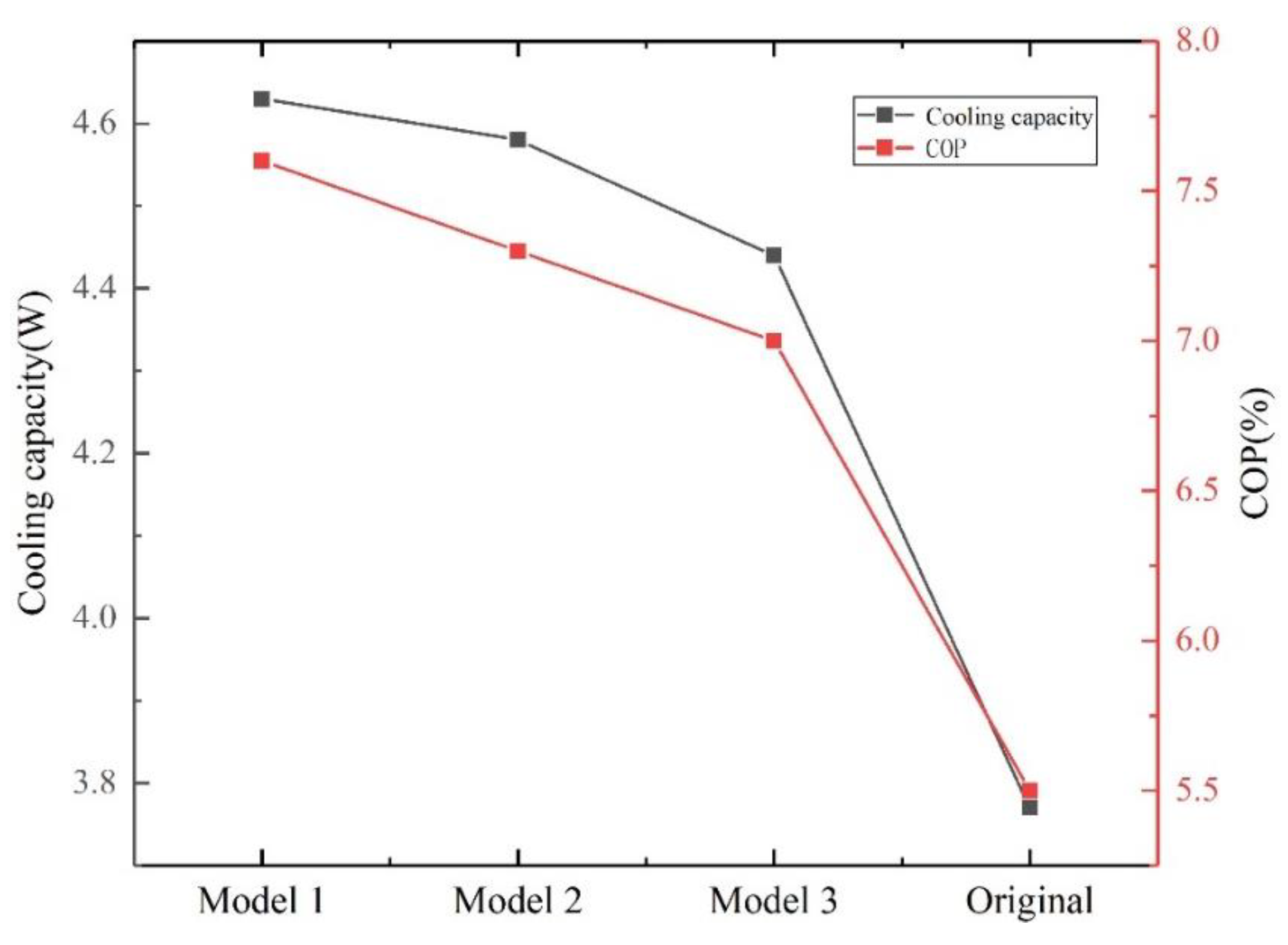
Figure 9 displays the cooling capacity and COP of the refrigerator at 120 K. The cooling capacity of the Original Model was 3.77 W, and the corresponding cooling capacities of Models 1, 2, and 3 were 4.63, 4.58, and 4.44 W, respectively. The COP of the Original Model was 5.5%, and the corresponding COP of Models 1, 2, and 3 were 7.6, 7.3, and 7.0%, respectively. Compared to the Original Model, Model 1 shows a significant improvement in both cooling capacity and COP. Model 1 had a smoother flow at the boundary owing to the conical tube transition at both ends of the pulse tube, and the hot and cold fluids were distributed uniformly in the pulse tube. Models 2 and 3 also show some improvement in cooling performance, but Model 2 is a little more effective. It shows that adding a partial conical pulse tube on the right side has a greater effect on flow and heat transfer than adding it on the left side while adding partial conical tubes on both sides of the pulse tube gives the best results. The boundary of the Original Model is easily disturbed by the unequal diameter of both sides of the pulse tube and the heat exchanger, which results in the mixing of hot and cold fluids and heat transfer from the hot fluid to the cold fluid, decreasing the cooling performance.
5. Conclusions
In this study, four two-dimensional simulation models of pulse tube refrigerator were built, and the velocity and temperature fields of adding a 45° conical tube on both sides of the pulse tube were compared and analyzed. The results demonstrated that the conical tube can effectively improve the multi-dimensional flow in the pulse tube and achieve a better cooling effect. The main conclusions are as follows:
(1) The Model 1 had the best cooling effect of the four models, with the lowest cooling temperature being 11.35 K lower than the Original Model.
(2) Compared with the original model, Model 1 can reduce the flow velocity at the entrance and exit of the pulse tube, and the vorticity at the boundary is small, which inhibits the generation and development of vortices and reduces the heat transfer losses due to vortices. Model 1 can better maintain the temperature gradient of the pulse tube, and the low temperature region, transition region, and high temperature region stratification is obvious while the original model high temperature region and transition region fluid mixing (cold and hot fluid mixing). Therefore, the addition of 45° tapered tubes on both sides of the pulse tube can improve the cooling capacity and COP of the refrigerator.
This model only requires the addition of 45° tapered tubes on both sides of the pulse tube without changing the diameter of the heat exchanger to achieve the suppression of disturbing flows. Therefore, it can be used to guide the design of pulse tube refrigerators.
Author Contributions
Methodology, W.S.; software, Y.M.; resources, W.J.; writing—original draft preparation, Y.M.; writing—review and editing, Z.C., W.S. and W.J.; project administration, W.S. All authors have read and agreed to the published version of the manuscript.
Funding
This research was funded by Taishan Scholar Project (Grand No. tsqn202103142), Natural Science Foundation of Shandong Province (No. ZR2021QE033) and China Postdoctoral Science Foundation (No. 2021M702013).
Data Availability Statement
Data is contained within the article.
Acknowledgments
This work was supported by the Taishan Scholar Project (Grand No. tsqn202103142), Natural Science Foundation of Shandong Province (No. ZR2021QE033) and China Postdoctoral Science Foundation (No. 2021M702013).
Conflicts of Interest
The authors declare no conflict of interest.
Nomenclature
| A0 | Maximum displacement | t | Time |
| CD | Taper pulse tube | Stress tensor | |
| CHX | Cold Heat Exchanger | Velocity | |
| COP | Coefficient of Performance | v | Viscosity |
| Ef | Fluid total energy | w | Angular frequency |
| Es | Solid total energy | WHX1 | Aftercooler |
| F | Body force | WHX2 | Hot heat exchanger |
| f | Frequency | ρf, ρ | Fluid density |
| kf, keff | Thermal conductivity | ρs | Solid density |
| P | Pressure | Φ | Porosity |
| S | Source term | ω | Vorticity |
| T | Temperature |
References
- Bian, S. Small Cryogenic Refrigerator; Mechanical Industry Press: Xi’an, China, 1983. [Google Scholar]
- Gifford, W.E.; Longsworth, R.C. Pulse tube refrigeration. J. Eng. Ind.-Trans. ASME 1964, 86, 264–270. [Google Scholar] [CrossRef]
- Longsworth, R.C. An Experimental Investigation of Pulse Tube Refrigeration Heat Pumping Rates. In Advances in Cryogenic Engineering; Springer: New York, NY, USA, 1967; pp. 608–618. [Google Scholar]
- Mikulin, E.I.; Tarasov, A.A.; Shkrebyonock, M.P. Low temperature expansion pulse tubes. Adv. Cryog. Eng. 1984, 29, 629–637. [Google Scholar]
- Radebaugh, R.; Zimmerman, J.; Smith, D.R. A comparison of three types of pulse tube refrigerators: New methods for reaching 60 K. Adv. Cryog. Eng. 1986, 31, 779–789. [Google Scholar]
- Kanao, K.; Watanabe, N.; Kanazawa, Y. A miniature pulse tube refrigerator for temperature below 100 K. Cryogenics 1994, 34, 167–170. [Google Scholar] [CrossRef]
- Cha, J.S.; Ghiaasiaan, S.M.; Desai, P.V. Multi-dimensional flow effects in pulse tube refrigerators. Cryogenics 2006, 46, 658–665. [Google Scholar] [CrossRef]
- Pang, X.; Dai, W.; Wang, X.; Ma, S. CFD investigation on the characteristics of annular pulse tube. Int. J. Refrig. 2020, 114, 181–188. [Google Scholar] [CrossRef]
- Dai, Q.; Chen, Y.; Yang, L. CFD investigation on characteristics of oscillating flow and heat transfer in 3D pulse tube. Int. J. Heat Mass Transf. 2015, 84, 401–408. [Google Scholar] [CrossRef]
- Yan, C.; Zhang, Y.; Qiu, J.; Chen, Y.; Wang, X.; Dai, W.; Ma, M.; Li, H.; Luo, E. Numerical and experimental study of partly tapered pulse tube in a pulse tube cryocooler—ScienceDirect. Int. J. Refrig. 2020, 120, 474–480. [Google Scholar] [CrossRef]
- Abolghasemi, M.A.; Stone, R.; Dadd, M.; Bailey, P.; Liang, K. Minimising flow losses within the pulse tube of a Stirling pulse tube cryocooler. IOP Conf. Ser. Mater. Sci. Eng. 2019, 502, 012044. [Google Scholar] [CrossRef]
- Ashwin, T.R.; Narasimham, G.; Jacob, S. CFD analysis of high frequency miniature pulse tube refrigerators for space applications with thermal non-equilibrium model. Appl. Therm. Eng. 2010, 30, 152–166. [Google Scholar] [CrossRef]
- He, Y.; Gao, C.; Xu, M.; Chen, Z.; Tao, W. Numerical simulation of convergent and divergent tapered pulse tube cryocoolers and experimental verification. Cryogenics 2001, 41, 699–704. [Google Scholar]
- Yang, L.W. Experimental research of high frequency tapered pulse tube cooler. Cryogenics 2009, 49, 738–741. [Google Scholar] [CrossRef]
- He, Y.L.; Zhao, C.F.; Ding, W.J.; Yang, W.W. Two-dimensional numerical simulation and performance analysis of tapered pulse tube refrigerator. Appl. Therm. Eng. 2007, 27, 1876–1882. [Google Scholar] [CrossRef]
- Zhu, S.W.; Nogawa, M.; Inoue, T. mAnalysis of DC gas flow in GM type double inlet pulse tube refrigerators. Cryogenics 2009, 49, 66–71. [Google Scholar] [CrossRef]
- Antao, D.S.; Farouk, B. Numerical simulations of transport processes in a pulse tube cryocooler: Effects of taper angle. Int. J. Heat Mass Transf. 2011, 54, 4611–4620. [Google Scholar] [CrossRef]
- Pang, X.; Chen, Y.; Wang, X.; Dai, W.; Luo, E. Numerical and experimental study of an annular pulse tube used in the pulse tube cooler. IOP Conf. Ser. Mater. Sci. Eng. 2017, 278, 012145. [Google Scholar] [CrossRef]
- Shiraishi, M.; Takamatsu, K.; Murakami, M.; Nakano, A. Dependence of convective secondary flow on inclination angle in an inclined pulse tube refrigerator revealed by visualization. Cryogenics 2004, 44, 101–107. [Google Scholar] [CrossRef]
- Liu, Y.W.; He, Y.L. A new tapered regenerator used for pulse tube refrigerator and its optimization. Cryogenics 2008, 48, 483–491. [Google Scholar]
- Sang, H.B.; Jeong, E.S.; Jeong, S. Two-dimensional model for tapered pulse tubes. Part 1: Theoretical modeling and net enthalpy flow. Cryogenics 2000, 40, 379–385. [Google Scholar]
- Sang, H.B.; Jeong, E.S.; Jeong, S. Two-dimensional model for tapered pulse tubes. Part 2: Mass streaming and streaming-driven enthalpy flow loss. Cryogenics 2000, 40, 387–392. [Google Scholar]
- Yin, C.L. CFD simulation of the gas flow in a pulse tube cryocooler with two pulse tubes. IOP Conf. Ser. Mater. Sci. Eng. 2015, 101, 012100. [Google Scholar] [CrossRef]
- Yin, C.; Chen, H.; Zhao, M.; Fei, Q.; Cai, J.; Li, Y. Experimental investigation of a u-shape pulse tube cryocooler with one regenerator and two pulse tubes. In Proceedings of the Aip Conference. American Institute of Physics, Spokane, WA, USA, 13–17 June 2012. [Google Scholar]
- Wang, K.; Zheng, Q.R.; Zhang, C.; Lin, W.S.; Lu, X.S.; Gu, A.Z. The experimental investigation of a pulse tube refrigerator with a ‘L’ type pulse tube and two orifice valves. Cryogenics 2006, 46, 643–647. [Google Scholar] [CrossRef]
- Fluent INC. Fluent 14.5 User Manual; Fluent INC: Canonsburg, PA, USA, 2012. [Google Scholar]
- Gu, C.; Zhou, Y.; Wang, J.; Ji, W.; Zhou, Q. CFD analysis of nonlinear processes in pulse tube refrigerators: Streaming induced by vortices. Int. J. Heat Mass Transf. 2012, 55, 7410–7418. [Google Scholar] [CrossRef]
Figure 1.
Four types of pulse tube structures. (a) Original Model. (b) Model 1. (c) Model 2. (d) Model 3.
Figure 1.
Four types of pulse tube structures. (a) Original Model. (b) Model 1. (c) Model 2. (d) Model 3.

Figure 2.
Comparison of simulation results with previously reported results.
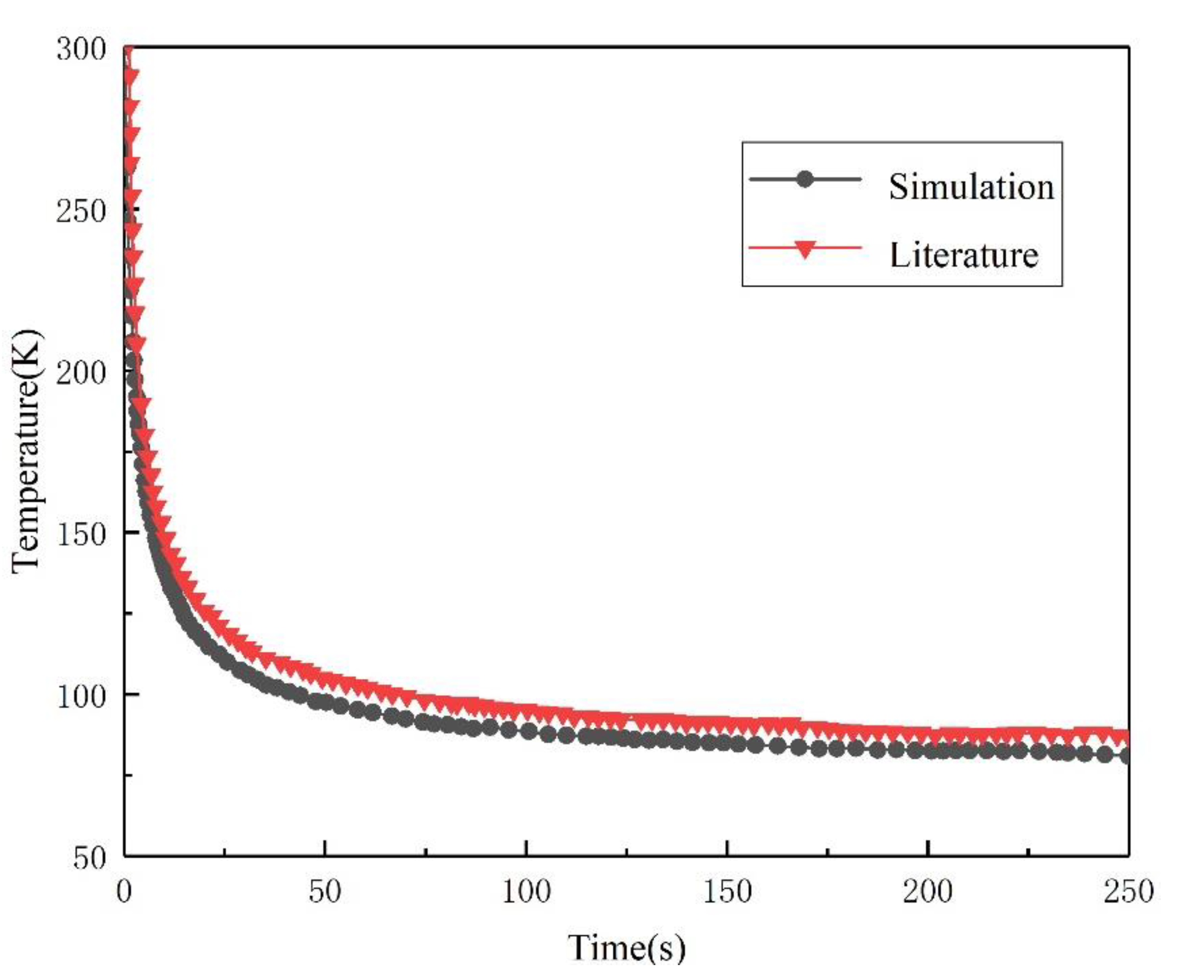
Figure 3.
Average minimum cooling temperatures of four models.
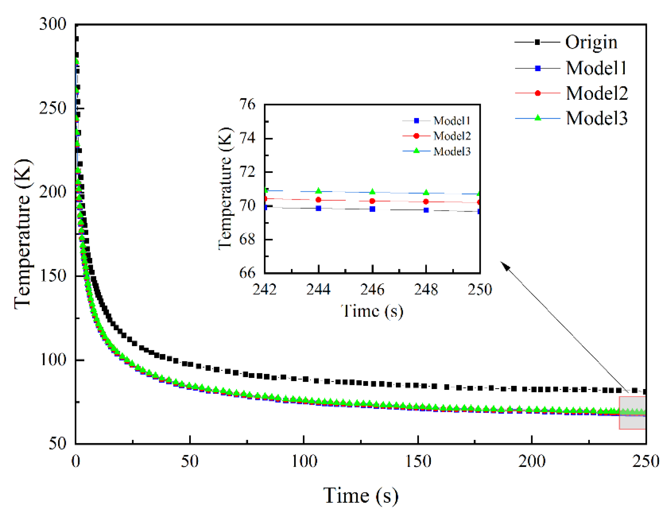
Figure 4.
Axial temperature variation of the pulse tube.
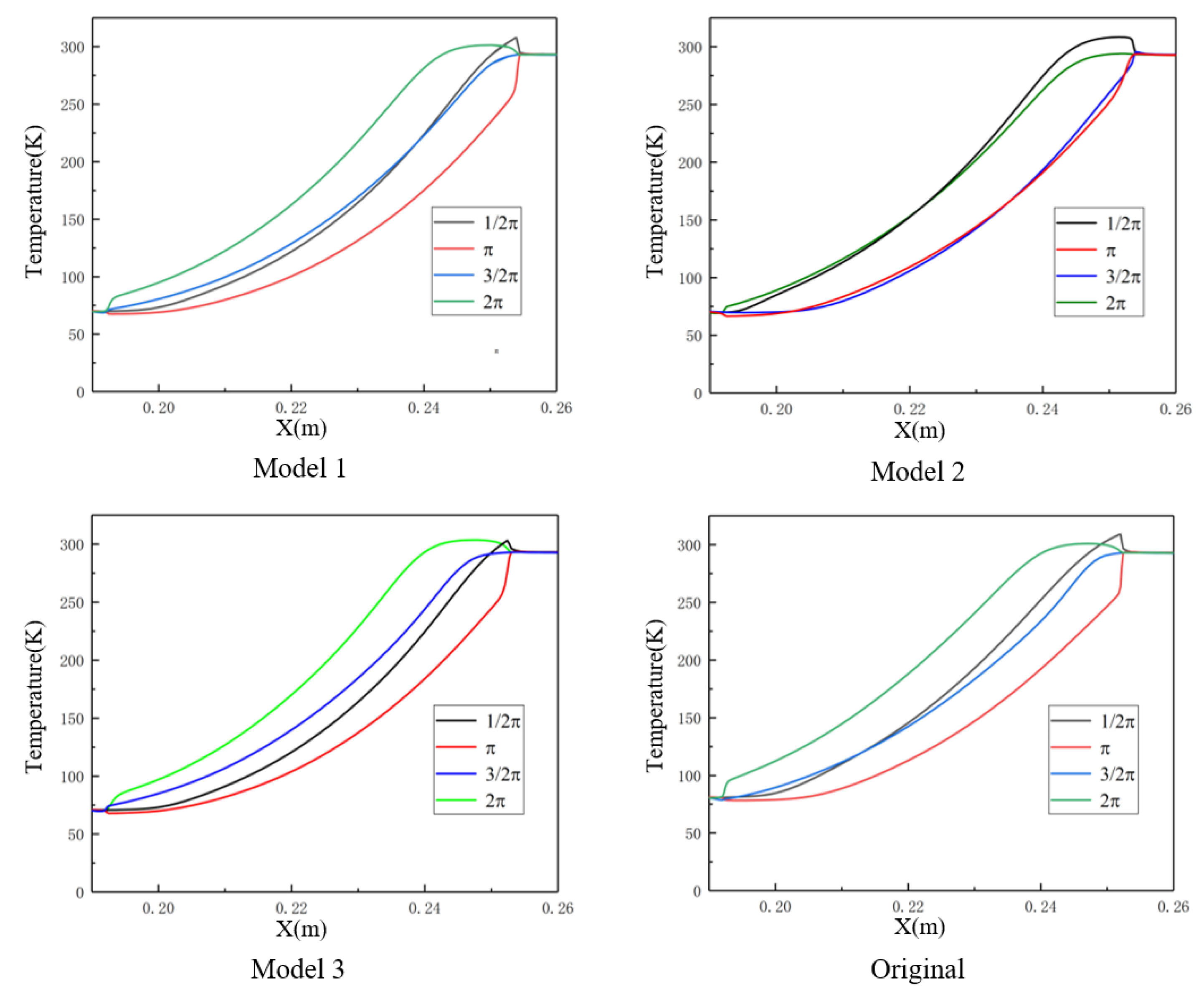
Figure 5.
Inlet and outlet speed amplitude.
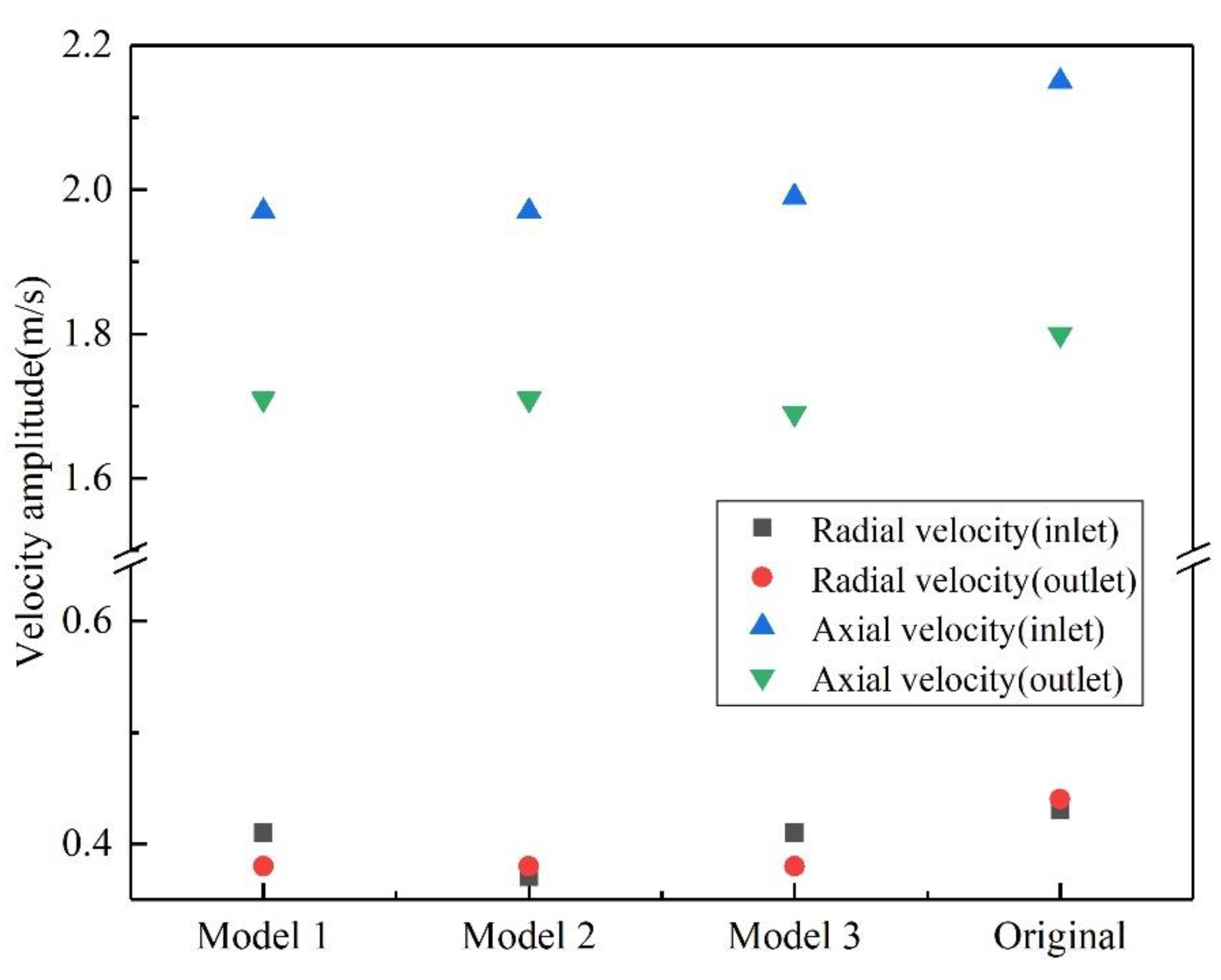
Figure 6.
Pulse tube temperature cloud.

Figure 7.
Pulse tube vorticity cloud.

Figure 8.
Pulse tube velocity vector diagram.

Figure 9.
Cooling capacity and COP at 120 K.

Table 1.
Geometry dimensions and boundary conditions.
| Components | Number | Radius (mm) | Length (mm) | Material | Boundary Conditions |
|---|---|---|---|---|---|
| Compressor | A | 9.54 | 7.5 | Steel | Adiabatic |
| Transfer line | B | 1.55 | 101 | Steel | Adiabatic |
| WHX1 | C | 4 | 20 | Copper | 300 K |
| Regenerator | D | 4 | 58 | Steel | Adiabatic |
| CHX | E | 3 | 5.7 | Copper | Adiabatic |
| Pulse tube | F | 2.5 | 60 | Steel | Adiabatic |
| WHX2 | G | 4 | 10 | Copper | 300 K |
| Inertance Tube | H | 0.425 | 684 | Steel | Adiabatic |
| gas reservoir | I | 13 | 130 | Steel | Adiabatic |
Disclaimer/Publisher’s Note: The statements, opinions and data contained in all publications are solely those of the individual author(s) and contributor(s) and not of MDPI and/or the editor(s). MDPI and/or the editor(s) disclaim responsibility for any injury to people or property resulting from any ideas, methods, instructions or products referred to in the content. |
© 2023 by the authors. Licensee MDPI, Basel, Switzerland. This article is an open access article distributed under the terms and conditions of the Creative Commons Attribution (CC BY) license (https://creativecommons.org/licenses/by/4.0/).
Share and Cite
MDPI and ACS Style
Meng, Y.; Cui, Z.; Shao, W.; Ji, W. Numerical Simulation of the Heat Transfer and Flow Characteristics of Pulse Tube Refrigerators. Energies 2023, 16, 1906. https://doi.org/10.3390/en16041906
AMA Style
Meng Y, Cui Z, Shao W, Ji W. Numerical Simulation of the Heat Transfer and Flow Characteristics of Pulse Tube Refrigerators. Energies. 2023; 16(4):1906. https://doi.org/10.3390/en16041906
Chicago/Turabian StyleMeng, Yuan, Zheng Cui, Wei Shao, and Wanxiang Ji. 2023. "Numerical Simulation of the Heat Transfer and Flow Characteristics of Pulse Tube Refrigerators" Energies 16, no. 4: 1906. https://doi.org/10.3390/en16041906
Note that from the first issue of 2016, this journal uses article numbers instead of page numbers. See further details here.