An Improved Microseismic Signal Denoising Method of Rock Failure for Deeply Buried Energy Exploration


1
School of Civil Engineering, Dalian University of Technology, Dalian 116024, China
2
School of Earth Sciences and Engineering, Hohai University, Nanjing 210098, China
*
Author to whom correspondence should be addressed.
Energies 2023, 16(5), 2274; https://doi.org/10.3390/en16052274
Submission received: 9 December 2022
/
Revised: 21 February 2023
/
Accepted: 23 February 2023
/
Published: 27 February 2023
Abstract
:Microseismic monitoring has become a well-known technique for predicting the mechanisms of rock failure in deeply buried energy exploration, in which noise has a great influence on microseismic monitoring results. We proposed an improved microseismic denoising method based on different wavelet coefficients of useful signal and noise components. First, according to the selection of an appropriate wavelet threshold and threshold function, the useful signal part of original microseismic signal was decomposed many times and reconstructed to achieve denoising. Subsequently, synthetic signals of different types (microseismic noise, microseismic current, microseismic noise current) and with various signal-to-noise ratios (SNRs, −10~10) were used as test data. Evaluation indicators (mean absolute error μ and standard deviation error σ) were established to compare the denoising effect of different denoising methods and verify that the improved method is more effective than the traditional denoising methods (wavelet global threshold, empirical mode decomposition and wavelet transform–empirical mode decomposition). Finally, the proposed method was applied to actual field microseismic data. The results showed that the microseismic signal (with different types of noise) could be fully denoised (car honk, knock, current and construction noise, etc.) without losing useful signals (pure microseismic), suggesting that the proposed approach provides a good basis for the subsequent evaluation and classification of rock burst disasters.
1. Introduction
As the global population continues to grow, the existing energy sources are characterized by high pollution levels and small reserves; therefore, the needs of humans cannot be met. There is an urgent need to expand new energy sources on a larger scale and deeper levels. One need is to continue mining energy sources such as coal, oil and gas in deeply buried formations [1,2,3,4], and another is to explore clean geothermal energy and build hydropower stations and diversion tunnels [5,6]. These engineering activities are often associated with complex geological conditions and high engineering difficulty, which could result in major disasters [7,8,9] such as collapse, rock burst and water inrush in deep rock masses, posing a threat to the safety of personnel and equipment, restricting the progress of engineering construction and increasing the potential for property losses. For example, 21 miners were killed in a rock burst accident at Longyun Coal Mine in China in October 2018 [10]. The extremely strong rock burst at the Jinping hydropower station caused considerable losses of personnel and property [11]. The largest recorded mine pressure was during a magnitude 5.5 event at the Werra River mine in Germany [12]. These accidents are attributed to rock failure caused by geostress disturbances. Therefore, studies of rock failure are of great value for energy exploration, and microseismic monitoring technology has been widely used in rock failure assessment and prediction in recent years [13,14,15]. Rock failure can generate microseismic signals, and researchers further analyze the failure characteristics of deep rocks through collected microseismic data. Since the magnitude of a microseismic signal is very weak, the noise generated by the external complex environment may drown out the original microseismic signal, leading to low-SNR data, which directly affects the accuracy of estimates of location and moment information for source mechanisms [16,17]. Therefore, finding an effective and reliable denoising method is a key step for assessing rock failure disasters in deeply buried energy exploration.
In previous denoising methods, the denoising effect of noisy microseismic signals was found to be affected by many factors, for example, the presence of random noise, low SNRs and algorithm selection [18,19]. Denoising methods are characterized by low applicability and are difficult to widely promote, which hinders the development of microseismic monitoring technology. Therefore, methods for denoising microseismic signals are constantly updated. Initially, the Fourier transform was introduced to transform the time domain into the frequency domain, and the useful information in the original signal was characterized by the frequency domain [20,21]. Based on the Fourier transform, filter denoising by setting a filter-specific frequency band and a short-time Fourier transform method with window were proposed [22,23,24,25]. However, they can only reflect the overall features and cannot fully reflect the local characteristics of the signal and the limitations of uncertainty; therefore, the methods based on the Fourier transform are more suitable for analyzing quasisteady signals. In view of the above defects, wavelet transform (WT) and empirical mode decomposition (EMD) were proposed to analyze nonstable signals [26,27,28]. EMD is a time–frequency analysis method that adaptively decomposes different types of signals into multiple intrinsic mode functions (IMFs) according to the time scale characteristics of the signal [29,30]. This approach provides better temporal and spatial resolutions than other method, but the EMD method is prone to problems such as mode aliasing, end effects and complicated termination criteria screening [31], which limit the accuracy of decomposition and the EMD method in microseismic signal processing in some cases.
In recent years, WT has become a powerful method for denoising different signals due to its time–frequency characteristics and multiresolution analysis characteristics [17,32]. In WT, a signal is decomposed into approximate information (low-frequency signal) and detailed information (high-frequency signal) through translation and scale extension of the mother wavelet; then, the information is reconstructed in a time–frequency localization analysis method with a time window and a frequency window [33,34,35,36]. Although the WT has advantages in decomposing noisy signals, it is difficult to determine the critical value of useful information and noise, which can lead to useful signals not being fully separated. Thus, more effective improved wavelet threshold methods were established [37,38]; they are mainly based on the use of different mother wavelets [39], decreasing empirical wavelet coefficients to suppress noise [40], and changing the traditional hard-and soft-value threshold functions [41].
The above methods mainly improve the signal-to-noise ratio (SNR) of specific noisy signals by improving parameter optimization in the selected denoising method and play a role in promoting the broad application of WT in shallow coal seams, rock strata and mining and extraction scenarios. However, in the actual process of deep energy exploration, the noise contained in the collected microseismic data is complex and disordered. It is difficult to decompose useful information and noise signals at multiple scales by only improving a single calculation parameter. Therefore, we study the applicability and effectiveness of an optimized wavelet threshold denoising method. We propose an improved signal denoising method based on a wavelet threshold to denoise deeply buried microseismic signals. According to the characteristics of the WT coefficient of microseismic singles, the original wavelet threshold function and parameters are optimized to evaluate the denoising results of different methods for synthetic microseismic data containing noise. The denoising effect of the improved method is analyzed based on microseismic signals with different SNRs, and the feasibility of the method in low-SNR cases is proven. Finally, with the microseismic data collected from an actual deep tunnel as examples, we verity that the method is more effective than the EDM and wavelet threshold methods and can remove different types of noise signals without losing useful signal information.
2. Materials and Methods
2.1. Engineering Background and Data Source
2.1.1. Engineering Background
To solve the major problem of urban and industrial water shortages around Xi’an City in Shaanxi Province, China (Figure 1a,b), the Hanjiang-to-Weihe River Diversion project was constructed to divert water from the Hanjiang River into the Weihe River to adjust the rational allocation of water resources in Shaanxi Province. The project is mainly composed of four parts: the Huangjinxia water control project, Huangjinxia to Sanhekou water transfer project, Sanhekou water control project and Qinling water conveyance tunnel. The Huangjinxia water control project is located 2000 m downstream of the main Hanjiang–Huangjinxia, and its main task is to retain the water level at the Hanjiang and power generation and transfer water from Huangjinxia Reservoir to the Huang-San tunnel. The Huang–Sanhekou water transfer project involves transporting Hanjiang water extracted from the Huangjinxia Pumping Station to Sanhekou Reservoir. The Sanhekou water control project is located 2000 m downstream of Sanhekou village, Daheba town, Foping County. It is mainly used to store water from the Ziwu River, and the main flow of Hanjiang is pumped into the reservoir by the pumping station. The water intake of the Qinling water conveyance tunnel is located at the confluence pool of Sanhekou Reservoir, and the water outlet is the Huangchi Ditch on the east side of Heihe, a tributary of the Weihe River. The task of the project is to transfer the diverted water from Hanjiang to the Guanzhong plain in the Weihe River Basin. The length of the Qinling water conveyance tunnel is 81.77 km, and the maximum burial depth of the tunnel is more than 2500 m. A tunnel boring machine (TBM) and drilling and blasting methods were employed during construction of the tunnel for 39.08 km and 42.69 km, respectively.
2.1.2. Dataset Sources
In the exploration of the deeply buried Qinling water conveyance tunnel, safety problems with large scopes and high concentrations readily occurred. For example, rock burst is caused by the collapse of the surrounding rock and fault failure. Therefore, the microseismic monitoring system of the Engineering Seismology Group (ESG) was used to monitor and prevent surrounding rock stability and deformation failure in real time (Figure 1c). The system comprises a Paladin digital signal acquisition system, a Hyperion digital signal processing system, six uniaxial sensors and signal transmission cables. The sensors were distributed along the axis of the tunnel, with three on the right sidewall and the other three on the left sidewall. When a seismic event occurs, each sensor collects different seismic signals, which are transmitted to the processing system through the optical fiber and stored as waveforms. In the complex construction environment, the detected microseismic signals contain different degrees and types of noise. Through signal analysis and research, it was confirmed that the waveforms of noisy microseismic signals can be basically divided into three categories: microseismic noise signals (Figure 2b), in the time-domain, submerged microseismic signals and low-SNR signals. In the obtained spectra, the main frequency bands of microseismic signals are not always clear, and noise causes intensive amplitude fluctuation, without clear spectral characteristics. For microseismic current signals (Figure 2c), in the time-domain, microseismic signals are relatively obvious, and the current characteristics are clear. In the corresponding spectra, the signal has no main frequency characteristics. For the current is seriously affected. For microseismic noise current signals (Figure 2d), in the time-domain, the microseismic information is not obvious, the SNR is low, and noise is abundant. The main frequency of microseismic event cannot be identified from a spectrum diagram, and the noise-related spectral features are obvious and distributed in multiple segments. Therefore, this study randomly selected 300 microseismic events monitored at the Hanjiang-to-Weihe River Diversion project from June to August 2021 for denoising.
2.2. The Proposed Method and Principle
Wavelet threshold denoising is a time-scale noise reduction method for signal analysis; it is a multiresolution analysis technique that can represent the local features of signals in both the time and frequency domains. It is a time–frequency localization analysis method based on a fixed window, and the wavelet shape, time window and frequency window can be changed. The low-frequency part of a signal has a low time resolution and a high frequency resolution, and the high-frequency part has a high time resolution and a low frequency resolution. This method is suitable for analyzing nonstationary signals and extracting the local characteristics of signals such as microseismic signals.
2.2.1. Principle of Wavelet Threshold Denoising
In general, the observed signal can be considered as follows [39]:
where f(t) is the observed signal, s(t) is the original signal and n(t) is the noise signal.
In most cases, microseismic signals are mainly concentrated at low-frequency bands, and noise signals are distributed at high-frequency bands. Therefore, after wavelet decomposition, the WT coefficient of the microseismic signal is larger than that of the noise. In processing, a suitable threshold is selected, and when the wavelet coefficient is less than the threshold, the wavelet is generated by the noise signal. If the coefficient is greater than the threshold, the wavelet is generated by the microseismic signal. After the wavelet coefficient is quantized based on the threshold for each layer, the high-frequency component and the low-frequency component of a microseismic signal are reconstructed based on inverse wavelet transform, thus effectively removing noise signal.
Therefore, the steps of wavelet threshold denoising are as follows:
- (1)
- Decomposition: Select the wavelet and determine the number of layers of wavelet decomposition.
- (2)
- Threshold processing: Select the threshold value and threshold function for nonlinear processing of wavelet coefficients.
- (3)
- Reconstruction: Use the new wavelet coefficients to reconstruct the signal and obtain the filtered signal.
2.2.2. Selection of Wavelet Threshold and Function
Traditional thresholds include fixed-form thresholds, adaptive thresholds, heuristic thresholds and minimax thresholds. However, these are fixed thresholds, and the corresponding amounts require large quantities of calculations and long operation run times; moreover, microseismic signal loss often occurs. To overcome these issues, threshold selection experiments were carried out based on a previously introduced method [39] to develop an improved threshold determination method:
where λ is the wavelet threshold, j is the decomposition scale, σ is the standard deviation of a noise signal and N is the length of the signal.
Equation (2) can be used to effectively distinguish, noise and microseismic signals. Notably, the threshold decreases with increasing decomposition scale, and the microseismic signal is retained to a great extent to remove noise.
Threshold denoising is performed based on the wavelet decomposition of a signal to obtain the high-frequency coefficients of each layer and the lowest low-frequency coefficients. Therefore, it is important to select an appropriate threshold function to filter the low-frequency coefficients. Donoho proposed traditional threshold function, namely, the soft threshold function and hard threshold function [43]. However, the soft threshold function yields a constant deviation between the reconstructed signal and the original signal, and the hard threshold function produces a step phenomenon.
Considering the above problems, an improved threshold function was designed. The threshold function, not just the soft threshold function, is continuous; as |x| increases, the deviation of y(x) and |x| decreases. The new threshold function is as follows:
where j is the decomposition scale. When |x|→λ, y(x)→0, the function is similar to the soft threshold function, and because the soft threshold function is continuous, there is no step phenomenon. When |x|→∞, y(x)→x, the function is similar to the hard threshold function and solving the soft threshold function always yields a certain deviation in results. In addition, the improved threshold function changes with the decomposition scale j, and thus, the adaptability to different decomposition levels is enhanced. Moreover, there are no uncertain parameters in the function; therefore, the stability of signal denoising is improved.
2.2.3. Improved Denoising Method
The improved denoising method is divided into the following steps. First, the sym4 wavelet is selected to decompose the signal into four levels based on the random nonstationary characteristics of the microseismic noise signal. Second, the improved threshold and threshold function are used for the nonlinear processing on the detailed components at each level of decomposition. Finally, the denoised microseismic signal is reconstructed based on the new wavelet coefficients.
The method flow is shown in Figure 3:
2.2.4. Parameter Selection
It is generally known that decomposition levels and the threshold function crucially influence the effectiveness of improved wavelet threshold denoising. For microseismic signals with noise [39], the number of decomposition layers is usually be set to 3–6. If the number of decomposition layers is larger, the effective signal and noise signal will be easy to separate into different frequency bands, resulting in the high-frequency portion of the effective signal being mistaken for noise and filtered. If number of decomposition levels is small, the original effective signal can be saved to a large extent, but the denoising effect may be poor. Therefore, a synthetic signal with a low SNR is analyzed as an example. The mean absolute error (μ) and standard deviation error (σ) are introduced as evaluation indicators to determine the optimal number of decomposition levels.
where di is the denoised signal, si is the real signal and N is the number of signal sampling points. μ is the degree to which the denoised signal matches the real signal, and the smaller μ is, the better the denoising effect. σ is the degree of dispersion of μ; the smaller σ is, the more concentrated the distribution of μ.
A comparative analysis of noise reduction is carried out for several groups of signals. The results show that when the number of decomposition layers is set to 4, μ and σ for the synthetic signal after denoising are minimized (Table 1), indicating that the noise reduction effect is good. Therefore, the optimal decomposition level is chosen as 4 in the denoising method.
According to the process of the wavelet threshold denoising method, the harmonic components of the signal with noise are decomposed into an approximate component dominated by the microseismic signal and a detailed component associated with both the noisy and useful parts of the signal. Therefore, it is necessary to perform hierarchical adaptive threshold denoising on the detailed component to filter and remove random noise. In the hard threshold method, the wavelet coefficients greater than the set threshold are output, and the coefficients less than the threshold are set to zero. In the soft threshold method, the wavelet coefficients less than the threshold are set to zero, and the wavelet coefficients greater than the threshold are reduced. Based on the shortcomings of the traditional hard threshold function and soft threshold function, the improved threshold function is adopted (Equation (3)). To verify the effectiveness of this function, the hard threshold, soft threshold [41] and improved wavelet threshold functions (Equation (3)) are used to denoise microseismic signals with different SNRs (5 dB, −2 dB and −10 dB), and μ and σ are calculated (Table 2).
When the SNR = 5, μ and σ for the improved threshold are minimized, and the effect of the improved threshold denoising method is the best (0.0041 < 0.0050 < 0.0109), as in the SNR decreases, when the microseismic signal is completely submerged in noise, obtained with the improved threshold method slightly increases, but it is still lower than those of the other two methods (0.0083 < 0.0107 < 0.0137). Due to the complex environment of the Hanjiang-to-Weihe River Diversion project, the SNR of microseismic signals with noise varies greatly; therefore, it is feasible to use the improved threshold function for denoising.
3. Results
To improve the efficiency of the study, first, the effectiveness of the improved method is tested by using synthetic data, and then the applicability of the improved method is verified by using actual microseismic noise data. The wavelet global threshold [44], EMD [30], EMD-WT [31] and improved wavelet threshold denoising methods are used for denoising tests with synthetic data.
3.1. Data and Evaluation Indicators
The synthetic data are derived from the superposition of the actual detected pure microseismic signals and different types of individual noise signals. After denoising, a denoised signal is compared with the original pure microseismic signal. When identifying the signal, it was found that the signal synthesized by pure microseismic and noise is very similar to the real microseismic noise signal. Therefore, the signals used in the data acquisition process effectively reflect signals in practical applications. That is, the actual monitored microseismic noise signals are composed of microseismic signal and noise signals. After removing the noise signals, the remaining signals are the microseismic signals.
Real monitored signals are irregular and nonstationary, and the signal waveforms are very complex and variable. Therefore, the pure microseismic signal and noise signal are superimposed to simulate a microseismic signal with noise. This approach can avoid the disadvantage of wavelet decomposition denoising with simulated signals, for which denoising can unrealistically effective. As shown in Figure 4, the microseismic noise signal, microseismic current signal and microseismic noise current signal were synthesized based on pure microseismic, noise and current signals. The microseismic signal information of associated with the synthesized signals underwent some changes. With the addition of noise, the local features were partially fused, the microseismic information was no longer obvious, and the SNR decreased. The synthesized signals encompass the features of all the noise signal samples in the monitored data. In most cases, the complex noise will change with time, and the corresponding frequency band will overlap with the frequency band of the microseismic signal; in some cases, the noise will completely hide the microseismic signal. In extreme cases, it is impossible for monitoring personnel to identify whether there is a real microseismic signal in a noisy signal; therefore, it is practical to reduce the noise in microseismic signals with low SNRs.
Based on the signal similarity, waveform changes and other factors, the denoised microseismic signal is compared to the pure microseismic signal in the synthetic signal. μ and σ are used as the evaluation indicators of denoising performance (Equations (4) and (5)). The smaller the value of μ is, the closer the denoised signal is to the pure microseismic signal. Additionally, the smaller the value of σ is, the closer the location of the microseismic signal after denoising is to zero.
3.2. Denoising Effect for Different Types of Synthetic Signals
The wavelet global threshold method, EMD, EMD-WT and improved wavelet threshold method were applied to denoise different synthesized signals. The results are shown in Figure 5, Figure 6, Figure 7, and μ and σ were calculated (Table 3).
During the denoising of the microseismic synthetic signals containing noise, part of the information of in the signals after denoising with the wavelet global threshold and EMD-WT method is lost. The amplitude and phase of the waveform are attenuated to different degrees. EMD displays the worst noise reduction effect, and this method is not effective for denoising; notably, the waveform of the microseismic signal after denoising has changed. The proposed improved wavelet threshold denoising method can better denoise and effectively filter the low- and high- voltage signals, and the denoised microseismic signals display highest similarity with the pure microseismic signals (Figure 5(a1,f1)).
The denoising of the synthesized microseismic signals with current information was explored (Figure 6), and the wavelet global threshold and EMD denoising methods do not effectively reduce the noise in these signals. Even the microseismic waveform is removed, resulting in only current interference noise after denoising. The EMD-WT denoising method can effectively reduce noise, but some microseismic information is not retained after denoising, and there is a distortion problem. However, the improved wavelet threshold denoising method can effectively remove the current information, retain a denoised microseismic signal that is similar to the pure microseismic signal, and highly denoise the low-voltage signal.
To assess the denoising effect of the synthetic microseismic signals with noise and current signals (Figure 7), the wavelet global threshold denoising method only removes the noise and retains the current noise; therefore, the denoising effect has limitations. EMD displays the worst denoising effect, except the noise is not effectively removed, and there is a large difference between the signal waveform after denoising and that of the pure microseismic signal. The EMD-WT method exhibits the phenomenon of the partial loss of microseismic information, and the size and number of signal amplitudes are significantly reduced. In addition, the positions without microseismic information are also incorrectly identified; therefore, useless signals are retained. The improved wavelet threshold denoising method can effectively retain the microseismic information and remove the mixed noise and current signals. The denoised microseismic signal displays the highest similarity with the pure microseismic signal.
Table 3 shows the values of μ and σ after denoising with different methods and different synthetic signal types. In each case, the values of the improved wavelet threshold denoising method are the smallest. μ and σ are 0.0217 and 0.0736, 0.0166 and 0.0447 and 0.0229 and 0.0791, respectively. In general, the improved method yields a high degree of microseismic information restoration and good integrity and produces a signal close to the pure microseismic signal. Additionally, this approach is suitable for the denoising of different types of noise.
3.3. Denoising Effect of Different SNR Synthetic Signals
The SNR is an important measure of signal quality, which is defined as the ratio of the magnitude of the useful signal to that of the noise signal (Equation (7)). A high SNR indicates that the real microseismic signal is significant, and the denoising effect is excellent.
where si is the original signal with noise, di is the signal after denoising and i is the sampling length.
The complexity of the environment influences the diversity of noise in an actual monitored signal. Especially for low-SNR microseismic data, the seismic phase is not obvious, and the noise waveform accounts for a large proportion of a signal. It is difficult to distinguish whether the real microseismic signal exists in a monitored signal waveform, and microseismic data processing may be distorted. We performed a denoising analysis of synthetic signals with different SNRs by synthesizing pure microseismic signals with different types of noise, such as construction noise, current interference and mixed noise. In this study, the SNR of the pure microseismic synthesized signals was set from −10 to 10 (with an interval of 1). There were 20 microseismic signals generated and a total of 60 synthetic signals. Then, the wave global threshold, EMD, EMD-WT and improved wavelet threshold denoising methods were used to denoise the 60 signals. Due to the similarity of the results, the certain SNRs (−10, −7, −4, and−2) were selected as examples. A comparison of the denoising results for synthetic signals processed with different methods is shown in Figure 8, Figure 9 and Figure 10.
For the microseismic noise signals with different SNRs, the wavelet global threshold method can effectively denoise the high SNR signals; the noise can be completely removed, and more important microseismic information can be identified. However, signals with low SNRs retain some noise (Figure 8(a1–d1)). No matter how the SNR changes, the EMD denoising method cannot effectively denoise signals, and the microseismic information is removed as noise (Figure 8(a2–d2)). After EMD-WT denoising at different SNRs, some useful signals are filtered and removed. The phenomenon of transition denoising occurs, resulting in the loss of parts of the original signal (Figure 8(a3–d3)). The denoising effect of the improved wavelet threshold method is the best. Notably, in cases with high- SNR signals, more detailed information from the microseismic signals is retained after denoising, the waveforms are closer to each other and the amplitude is almost unchanged (Figure 8(a4–d4)).
For microseismic current signals with different SNRs, the wavelet global threshold and EMD methods cannot effectively denoise the signals, mainly due to current interference; specifically, the current is not recognized as noise and is removed. In particular, the useful signal after EMD denoising changes (Figure 9(a2–d2)). EMD-WT can effectively denoise the synthesized microseismic current signal, and the current-related noise is removed; however, the recognition of microseismic signal information needs to be improved, and some details are not retained. The improved wavelet threshold approach can effectively denoise synthesized microseismic current signals with different SNRs (Figure 9(a3–d3)). If the current is not effectively removed, different degrees of current interference can affect the recognition of microseismic information in the synthetic signals, and the denoising effect is generally poor (Figure 9(a4–d4)).
For microseismic signals with noise, current and different SNRs (Figure 10), as the SNR increases, the denoising ability of the wavelet global threshold increases; that is, a synthetic signal with a low SNR cannot be effectively denoised, and the microseismic information changes after denoising. EMD displays no denoising ability. The EMD-WT results are similar to those in Figure 8 and Figure 9 and show the phenomenon of transition denoising; additionally, the original signal cannot be completely preserved. The improved wavelet threshold method displays the strongest denoising ability and the best denoising effect; it not only filters out and removes the mixed noise but also retains as much useful microseismic information as possible.
Based on the denoising of synthetic signals (with construction noise, current interference and mixed noise) with different SNRs, we observed that the signals denoised with the improved wavelet threshold method are the closest to the original signals. Furthermore, we plot the variations in μ and σ as the SNR decreases, as shown in Figure 11. As the SNR decreases, μ and σ for the improved wavelet threshold, EMD-WT, EMD and wavelet global threshold denoising methods increase. Surprisingly, the improved wavelet threshold yields the smallest μ and σ, and their changes are smoother. In contrast, for the wavelet global threshold and EMD methods, μ and σ are much larger than those for the improved wavelet threshold method, and the rate of change is larger when denoising different synthetic signals. Although the μ value for of EMD-WT is relatively small, the attenuation of σ is significant with decreasing SNR. It is confirmed that the improved wavelet threshold method provides sufficient denoising ability to adapt to signals with different SNRs.
4. Discussion
To verify the effectiveness and reliability of the improved method for deep microseismic noise, engineering and microseismic data with noise recorded at the Qinling water conveyance tunnel from June to August 2021 were selected. Different methods were used to denoise the signal, and the denoised signals were converted to the frequency domain by fast Fourier transform method for comparison [16].
For the actual monitoring data, the improved wavelet threshold method achieved a better denoising effect than the other three methods (Figure 12, Figure 13 and Figure 14). In the time domain, different types of noise were effectively filtered, and the extraction and recognition ability of microseismic information was strong; notably, the resulting waves displayed shapes similar to those of the real microseismic waves considered. After denoising, the time domain waveform was transformed into a spectrogram (Figure 12e, Figure 13e and Figure 14e), and there was a clear main frequency feature, which was similar to the main frequency feature of the pure microseismic signals (Figure 2a). EMD-WT displays obvious differences in denoising ability for different types of noise; it completely removes the current interference noise, but its ability to remove excessive construction noise was generally poor. The useful signal after denoising exhibited distortion, and the spectrum characteristics of the waveform displayed spectrum aliasing effects. Although EMD exhibited a certain denoising ability, the denoised signal still displayed a certain degree of noise; there were differences in the denoising of different types of noisy microseismic wave shapes, and the actual application of this approach was poor. The wavelet global threshold method could not denoise the microseismic signal containing current, and the spectrum characteristics did not change after denoising.
To further assess the obtained microseismic information, the SNR, mean squared error (MSE) and correlation coefficient (r) were established to evaluate the signal quality before and after denoising (Table 4).
MSE is defined as the expected value of the difference between the denoised signal and the true signal. If the MSE is smaller after denoising than before, the effect of denoising is good.
where r is defined as a statistical index of the relationship between the denoising signal and real signal. r reflects the degree of similarity between the time-domain and actual waveforms. If r is larger after noise reduction, the time-domain waveform similarity of the signal after denoising is high, and the effect of denoising is satisfactory.
where si is the true signal, di is the denoised signal, is the true signal mean, is the denoised signal mean and N is the number of sample points.
As shown in Table 4, compared with other denoising methods, the improved wavelet threshold method yields SNR and r values after i denoising that are significantly larger because it can effectively improve the signal quality. The signals before and after denoising display a strong correlation, and the microseismic information is retained to a large extent. However, the MSE is small, indicating that the signal after improved wavelet threshold denoising is similar to the original pure microseismic signal.
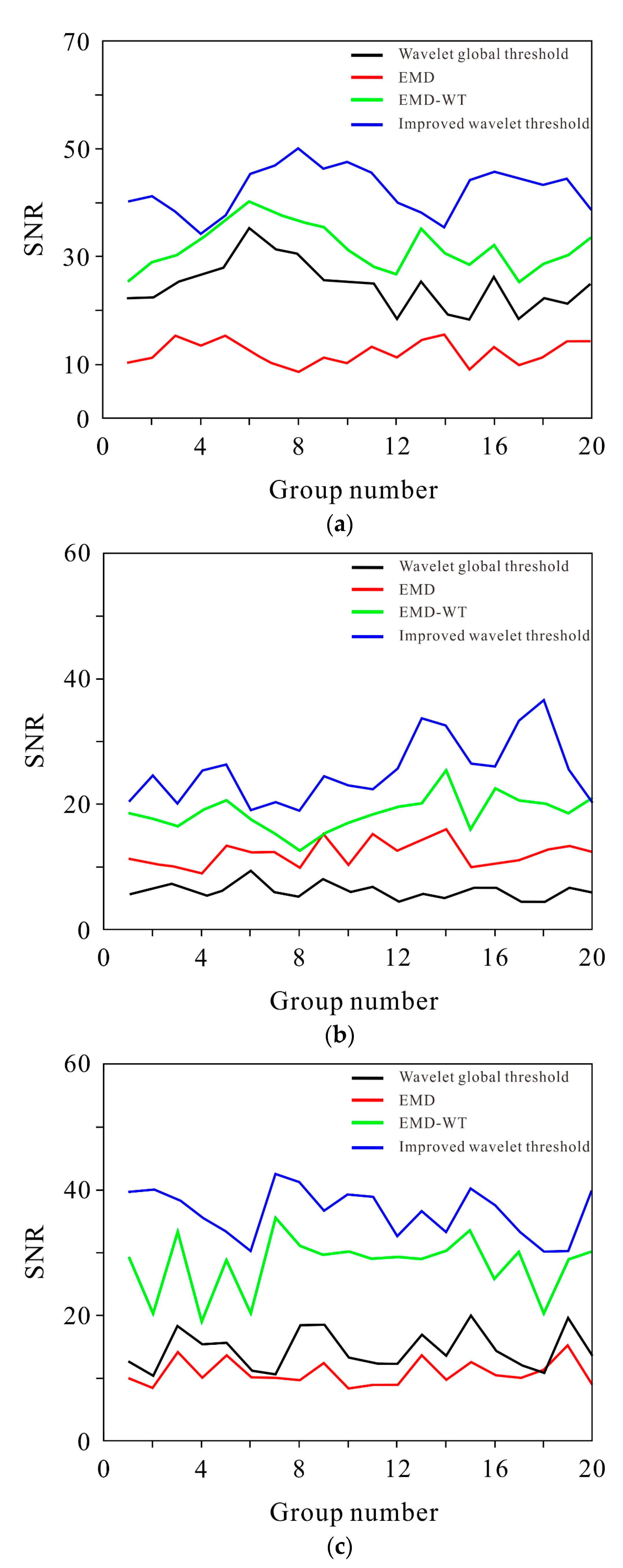
Finally, we randomly selected 300 microseismic data with different noise types for denoising, with 100 data of each type, and the mean value of the SNR after denoising was calculated for each group of 5. Overall, 20 groups were analyzed and evaluated. As shown in Figure 15, the actual monitored microseismic signals were denoised using the wavelet global threshold, EMD and EMD-WT methods. The distribution of the SNR displayed a gradient distribution. Among them, the SNR with denoising by the improved wavelet threshold method was the largest, which was in the first echelon of 34~50, 19~37 and 30~43. This result suggests that the improved wavelet threshold denoising method can effectively improve the SNR of signals and further confirms that the improved method has strong engineering practical application value for actual deep energy exploration.
5. Conclusions
In this paper, an improved denoising method is presented to analyze the different microseismic signals, and indicators are established to evaluate the relationship between the denoised signals and pure microseismic signals. The reliability and effectiveness of the proposed denoising method verified with an actual engineering monitoring data set. The following conclusions are obtained:
- (1)
- Through a threshold selection test, the improved threshold criterion was used to vary the wavelet threshold with changes in the decomposition scale, and the microseismic and noise signal components were effectively distinguished. The new threshold function overcame the step phenomenon and value deviation issues of the traditional threshold function. The number of decomposition levels was determined based on an evaluation index to reduce signal distortion.
- (2)
- Compared with the wavelet global threshold, EMD and EMD-WT methods, the improved wavelet threshold denoising method displayed better denoising performance for different types of synthetic signals with different SNRs. It overcomes or effectively makes up for the shortcomings of other methods, such as losing some useful information, retaining noise-related information and yielding invalid denoising results.
- (3)
- The denoising evaluation of real microseismic signals further shows that the proposed method can remove different types of noise, significantly improve the SNR of microseismic data, and restore the microseismic information to the greatest extent. The method proposed in this paper greatly promotes the optimization of microseismic denoising for complex, deeply buried, energy exploration.
Author Contributions
Conceptualization, S.T. and S.D.; methodology, S.T., S.D. and J.L.; validation, C.Z. and L.C.; investigation, S.T. and S.D.; data curation, J.L. and L.C.; writing—original draft preparation, S.D.; writing—review and editing, S.T. and C.Z.; supervision, S.T.; funding acquisition, S.T. All authors have read and agreed to the published version of the manuscript.
Funding
This work was supported by the National Natural Science Foundation of China (Grant Nos. 51874065 and U1903112).
Data Availability Statement
Not applicable.
Conflicts of Interest
The authors declare that there are no conflict of interest.
References
- Wang, Q.H.; Zhang, Y.T.; Xie, Z.; Zhao, Y.W.; Zhang, C.; Sun, C.; Wu, G.H. The Advancement and Challenges of Seismic Techniques for Ultra-Deep Carbonate Reservoir Exploitation in the Tarim Basin of Northwestern China. Energies 2022, 15, 7653. [Google Scholar] [CrossRef]
- Moscariello, A. Exploring for geo-energy resources in the Geneva Basin (Western Switzerland): Opportunities and challenges. Swiss Bull. Angew. Geol. 2019, 24, S105–S124. [Google Scholar]
- Wang, J.X.; Tang, S.B. Novel Transfer Learning Framework for Microseismic Event Recognition between Multiple Monitoring Projects. Rock Mech. Rock Eng. 2022, 55, 3563–3582. [Google Scholar] [CrossRef]
- Tang, S.B.; Li, J.M.; Ding, S.; Zhang, L.T. The influence of water-stress loading sequences on the creep behavior of granite. Bull. Eng. Geol. Environ. 2022, 81, 482. [Google Scholar] [CrossRef]
- Wójcik, K.; Zacharski, J.; Łojek, M.; Wróblewska, S.; Kiersnowski, H.; Waśkiewicz, K.; Wójcicki, A.; Laskowicz, R.; Sobień, K.; Peryt, T.; et al. New Opportunities for Oil and Gas Exploration in Poland—A Review. Energies 2022, 15, 1739. [Google Scholar] [CrossRef]
- Liang, X.; Tang, S.B.; Tang, C.A.; Hu, L.H.; Chen, F. Influence of water on the mechanical properties and failure behaviors of sandstone under triaxial compression. Rock Mech. Rock Eng. 2023, 56, 1131–1162. [Google Scholar] [CrossRef]
- Li, J.M.; Li, K.Y.; Tang, S.B. Automatic arrival-time picking of P-and S-waves of microseismic events based on object detection and CNN. Soil Dyn. Earthq. Eng. 2023, 64, 107560. [Google Scholar] [CrossRef]
- Keneti, A.; Sainsbury, B.A. Review of published rockburst events and their contributing factors. Eng. Geol. 2018, 246, 361–373. [Google Scholar] [CrossRef]
- Li, J.M.; Tang, S.B.; Song, H.B.; Chen, X.J. Engineering properties and microstructure of expansive soil treated with nanographite powder. J. Central South Univ. 2022, 29, 499–514. [Google Scholar] [CrossRef]
- Jiang, Y.D.; Zhao, Y.X.; Wang, H.W.; Zhu, J. A review of mechanism and prevention technologies of coal bumps in China. J. Rock Mech. Geotech. Eng. 2017, 9, 180–194. [Google Scholar] [CrossRef]
- Chen, B.R.; Feng, X.T.; Li, Q.P.; Luo, R.Z.; Li, S.J. Rock burst intensity classification based on the radiated energy with damage intensity at Jinping II hydropower station, China. Rock Mech. Rock Eng. 2015, 48, 289–303. [Google Scholar] [CrossRef]
- Tang, S.B.; Wang, J.X.; Chen, P.Z. Theoretical and numerical studies of cryogenic fracturing induced by thermal shock for reservoir stimulation. Int. J. Rock Mech. Min. Sci. 2020, 125, 104160. [Google Scholar] [CrossRef]
- Ma, T.H.; Tang, C.A.; Tang, S.B.; Kuang, L.; Yu, Q.; Kong, D.Q.; Zhu, X. Rockburst mechanism and prediction based on microseismic monitoring. Int. J. Rock Mech. Min. Sci. 2018, 110, 177–188. [Google Scholar] [CrossRef]
- Tang, S.B.; Wang, J.X.; Tang, C.A. Identification of microseismic events in rock engineering by a convolutional neural network combined with an attention mechanism. Rock Mech. Rock Eng. 2021, 54, 47–69. [Google Scholar] [CrossRef]
- Zhang, C.; Jin, G.; Liu, C.; Li, S.; Xue, J.; Cheng, R.; Wnag, X.; Zheng, X. Prediction of rockbursts in a typical island working face of a coal mine through microseismic monitoring technology. Tunn. Undergr. Space Technol. 2021, 113, 103972. [Google Scholar] [CrossRef]
- Zhang, W.; Feng, X.T.; Bi, X.; Yao, Z.B.; Xiao, Y.X.; Hu, L.; Niu, W.J.; Feng, G.L. An arrival time picker for microseismic rock fracturing waveforms and its quality control for automatic localization in tunnels. Comput. Geotech. 2021, 135, 104175. [Google Scholar] [CrossRef]
- Li, H.L.; Tuo, X.G.; Wang, R.L.; Courtois, J. A reliable strategy for improving automatic first arrival picking of high noise three component microseismic data. Seismol. Res. Lett. 2019, 90, 1336–1345. [Google Scholar] [CrossRef]
- Zhou, Y.; Wu, G. Unsupervised machine learning for waveform extraction in microseismic denoising. J. Appl. Geophys. 2020, 173, 103879. [Google Scholar] [CrossRef]
- Anvari, R.; Siahsar, M.A.N.; Gholtashi, S.; Kahoo, A.R.; Mohammadi, M. Seismic random noise attenuation using synchrosqueezed wavelet transform and low-rank signal matrix approximation. IEEE Trans. Geosci. Remote Sens. 2017, 55, 6574–6581. [Google Scholar] [CrossRef]
- Lu, C.P.; Dou, L.M.; Zhang, N.; Xue, J.H.; Wang, X.N.; Liu, H.; Zhang, J.W. Microseismic frequency-spectrum evolutionary rule of rockburst triggered by roof fall. Int. J. Rock Mech. Min. Sci. 2013, 64, 6–16. [Google Scholar] [CrossRef]
- Lu, C.-P.; Dou, L.-M.; Liu, B.; Xie, Y.-S.; Liu, H.-S. Microseismic low-frequency precursor effect of bursting failure of coal and rock. J. Appl. Geophys. 2012, 79, 55–63. [Google Scholar] [CrossRef]
- Griffin, D.; Lim, J. Signal estimation from modified short-time Fourier transform. IEEE Trans. Acoust. Speech Signal Process. 1984, 32, 236–243. [Google Scholar] [CrossRef]
- Reddy, B.S.; Chatterji, B.N. An FFT-based technique for translation, rotation, and scale-invariant image registration. IEEE Trans. Image Process. 1996, 5, 1266–1271. [Google Scholar] [CrossRef] [Green Version]
- Mirković, D.; Mahasoom, R.; Johnsson, L. An adaptive software library for fast fourier transforms. In Proceedings of the 14th International conference on Supercomputing, New York, NY, USA, 8–11 May 2000; pp. 215–224. [Google Scholar]
- Feichtinger, H.G.; Strohmer, T. Gabor Analysis and Algorithms: Theory and Applications; Springer Science & Business Media: Berlin/Heidelberg, Germany, 2012. [Google Scholar]
- Morlet, J.; Arens, G.; Fourgeau, E.; Giard, D. Wave propagation and sampling theory, Part I: Complex signal land scattering in multilayer media. Geophysics 1982, 47, 203–221. [Google Scholar] [CrossRef] [Green Version]
- Chun-Lin, L. A tutorial of the wavelet transform. NTUEE Taiwan 2010, 21, 22. [Google Scholar]
- Boudraa, A.O.; Cexus, J.C. EMD-Based Signal Filtering. IEEE Trans. Instrum. Meas. 2007, 56, 2196–2202. [Google Scholar] [CrossRef]
- Huang, N.E.; Shen, Z.; Long, S.R.; Wu, M.C.; Shih, H.H.; Zheng, Q.; Yen, N.C.; Tung, C.C.; Liu, H.H. The empirical mode decomposition and the Hilbert spectrum for nonlinear and non-stationary time series analysis. Proc. R. Soc. A 1998, 454, 903–995. [Google Scholar] [CrossRef]
- Hassan, H.H. Empirical mode decomposition (EMD) of potential field data: Airborne gravity data as an example. In SEG Technical Program Expanded Abstracts 2005; Society of Exploration Geophysicists: Tulsa, OK, USA, 2005; pp. 704–706. [Google Scholar]
- Kabir, M.A.; Shahnaz, C. Denoising of ECG signals based on noise reduction algorithms in EMD and wavelet domains. Biomed. Signal Process. Control 2012, 7, 481–489. [Google Scholar] [CrossRef]
- Mousavi, S.M.; Langston, C.A.; Horton, S.P. Automatic microseismic denoising and onset detection using the synchrosqueezed continuous wavelet transform. Geophysics 2016, 81, V341–V355. [Google Scholar] [CrossRef]
- Pan, Q.; Zhang, L.; Dai, G.; Zhang, H. Two denoising methods by wavelet transform. IEEE T Signal Process. 1999, 47, 3401–3406. [Google Scholar] [CrossRef] [Green Version]
- Starck, J.L.; Fadili, J.; Murtagh, F. The undecimated wavelet decomposition and its reconstruction. IEEE Trans. Image Process. 2007, 16, 297–309. [Google Scholar] [CrossRef] [PubMed] [Green Version]
- Cheng, H.; Yuan, Y.; WANG, E.D.; Fu, J.F. Study of hierarchical adaptive threshold micro-seismic signal denoising based on wavelet transform. J. Northeast. Univ. 2018, 39, 1332. [Google Scholar]
- Liang, Z.; Xue, R.; Xu, N.; Li, W. Characterizing rockbursts and analysis on frequency-spectrum evolutionary law of rockburst precursor based on microseismic monitoring. Tunn. Undergr. Space Tech. 2020, 105, 103564. [Google Scholar] [CrossRef]
- Shi, Y.; Zhang, D.; Ji, H.; Dai, R. Application of Synchrosqueezed Wavelet Transform in Microseismic Monitoring of Mines. IOP Conf. Ser. Earth Environ. Sci. 2019, 384, 012075. [Google Scholar] [CrossRef]
- Xie, B.; Shi, F.; Ma, S.; Li, F. Automatic picking method of microseismic signal first arrival time based on empirical wavelet transform. IOP Conf. Ser. Earth Environ. Sci. 2020, 44, 052055. [Google Scholar] [CrossRef] [Green Version]
- Li, H.L.; Shi, J.H.; Li, L.J.; Tuo, X.G.; Qu, K.; Rong, W.Z. Novel Wavelet Threshold Denoising Method to Highlight the First Break of Noisy Microseismic Recordings. IEEE T. Geosci. Remote 2022, 60, 5910110. [Google Scholar] [CrossRef]
- Mohammadi, S.; Leventouri, T. A study of wavelet-based denoising and a new shrinkage function for low-dose CT scans. Biomed. Phys. Eng. Expr. 2019, 5, 035018. [Google Scholar] [CrossRef]
- Cao, J.J.; Cai, Z.C.; Liang, W.Q. A novel thresholding method for simultaneous seismic data reconstruction and denoising. J. Appl. Geophys. 2020, 177, 104027. [Google Scholar] [CrossRef]
- Li, J.; Tang, S.; Li, K.; Zhang, S.; Tang, L.; Cao, L.; Ji, F. Automatic recognition and classification of microseismic waveforms based on computer vision. Tunn. Undergr. Space Technol. 2022, 121, 104327. [Google Scholar] [CrossRef]
- Donoho, D.L. De-noising by soft-thresholding. IEEE Trans. Inform. Theory 1995, 41, 613–627. [Google Scholar] [CrossRef] [Green Version]
- Dixit, A.; Majumdar, S. Comparative analysis of Coiflet and Daubechies wavelet using global TRhreshold for image de-noising. Int. J. Adv. Eng. Technol. 2013, 6, 2247–2252. [Google Scholar]
Figure 1.
(a,b) Geographical location/layout map of the Hanjiang-to-Weihe River diversion project [42], (c) Microseismic monitoring system of the Engineering Seismology Group.
Figure 1.
(a,b) Geographical location/layout map of the Hanjiang-to-Weihe River diversion project [42], (c) Microseismic monitoring system of the Engineering Seismology Group.
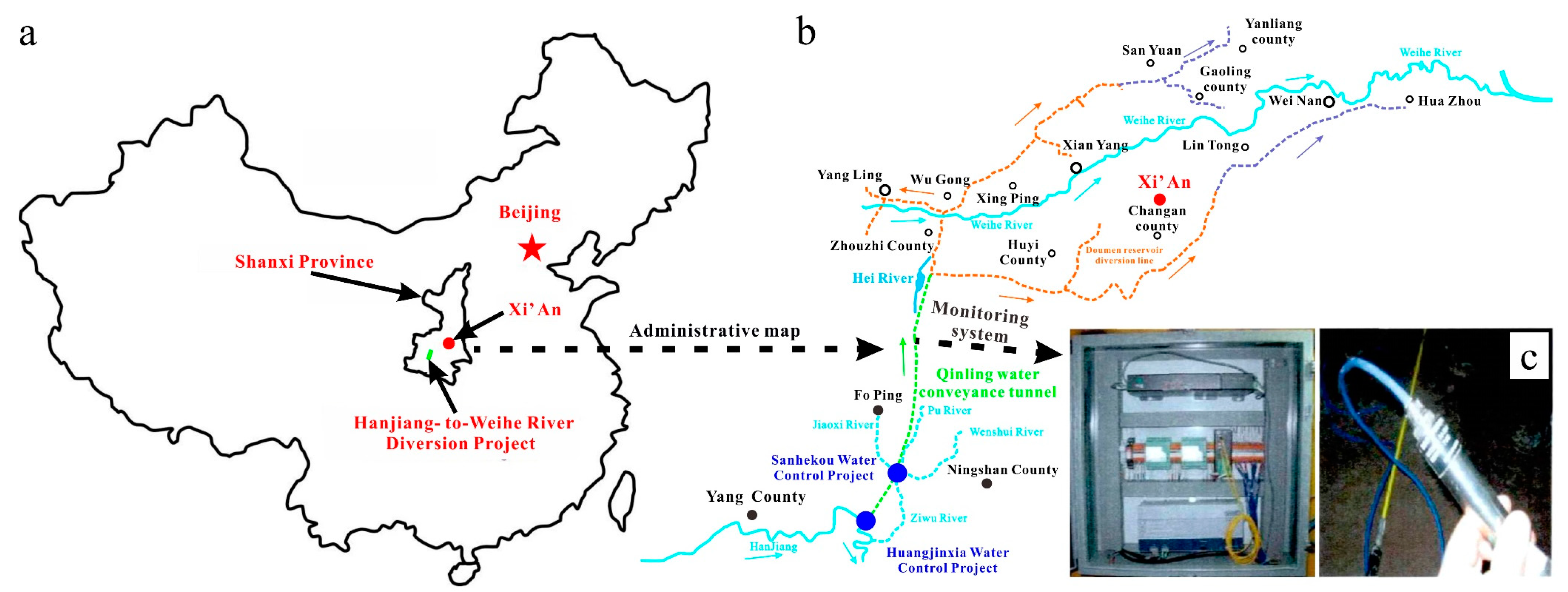
Figure 2.
Waveforms of different signals: (a) microseismic signal, (b) microseismic noise signal, (c) microseismic current signal, (d) microseismic noise current signal.
Figure 2.
Waveforms of different signals: (a) microseismic signal, (b) microseismic noise signal, (c) microseismic current signal, (d) microseismic noise current signal.

Figure 3.
Method flow, the {CAj,k} is approximate component and {CDj,k} is detailed component.
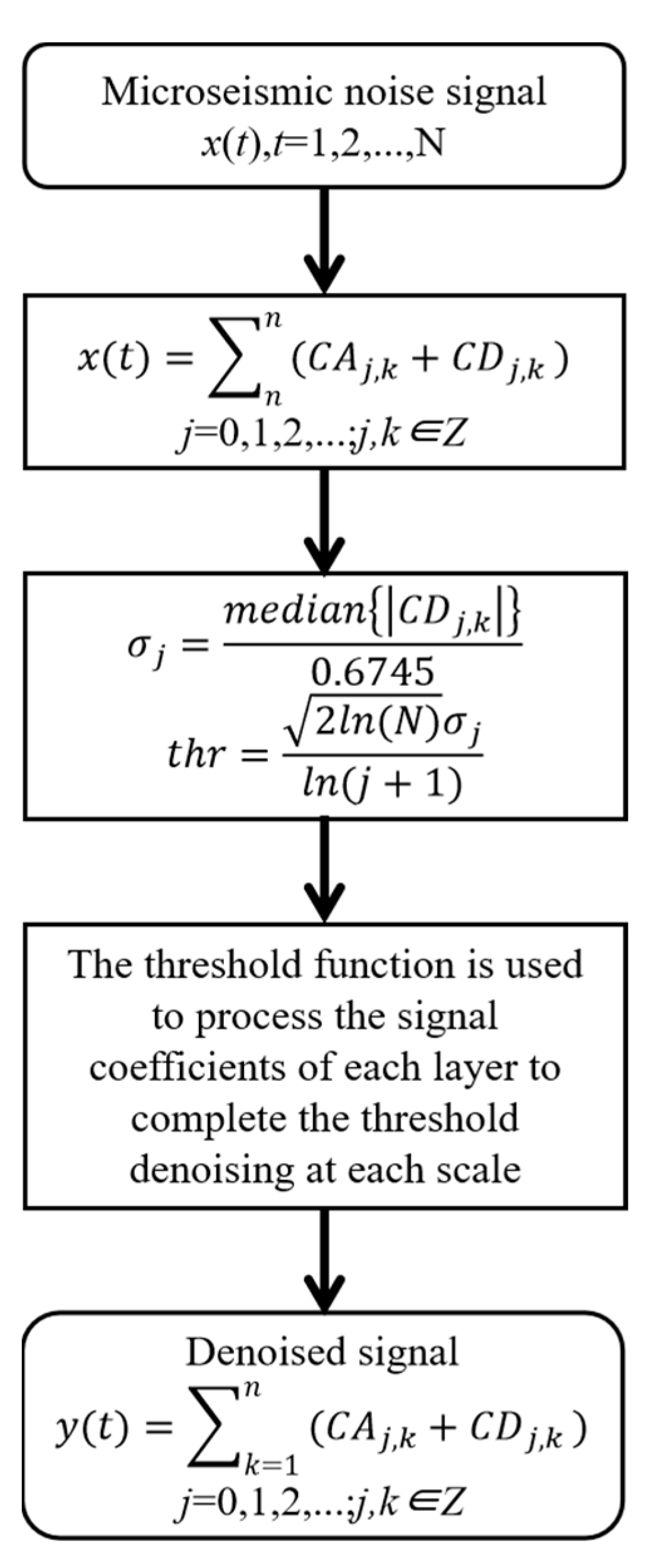
Figure 4.
Synthesized signal with microseismic, noise and current.

Figure 5.
Comparison of the denoising results of different methods for noise-containing synthetic microseismic signal: (a,a1) microseismic signal, (b,b1) microseismic noise signal, (c,c1) Wavelet global threshold denoising signal, (d,d1) EMD denoising signal, (e,e1) EMD-WT denoising signal, (f,f1) improved wavelet threshold denoising signal.
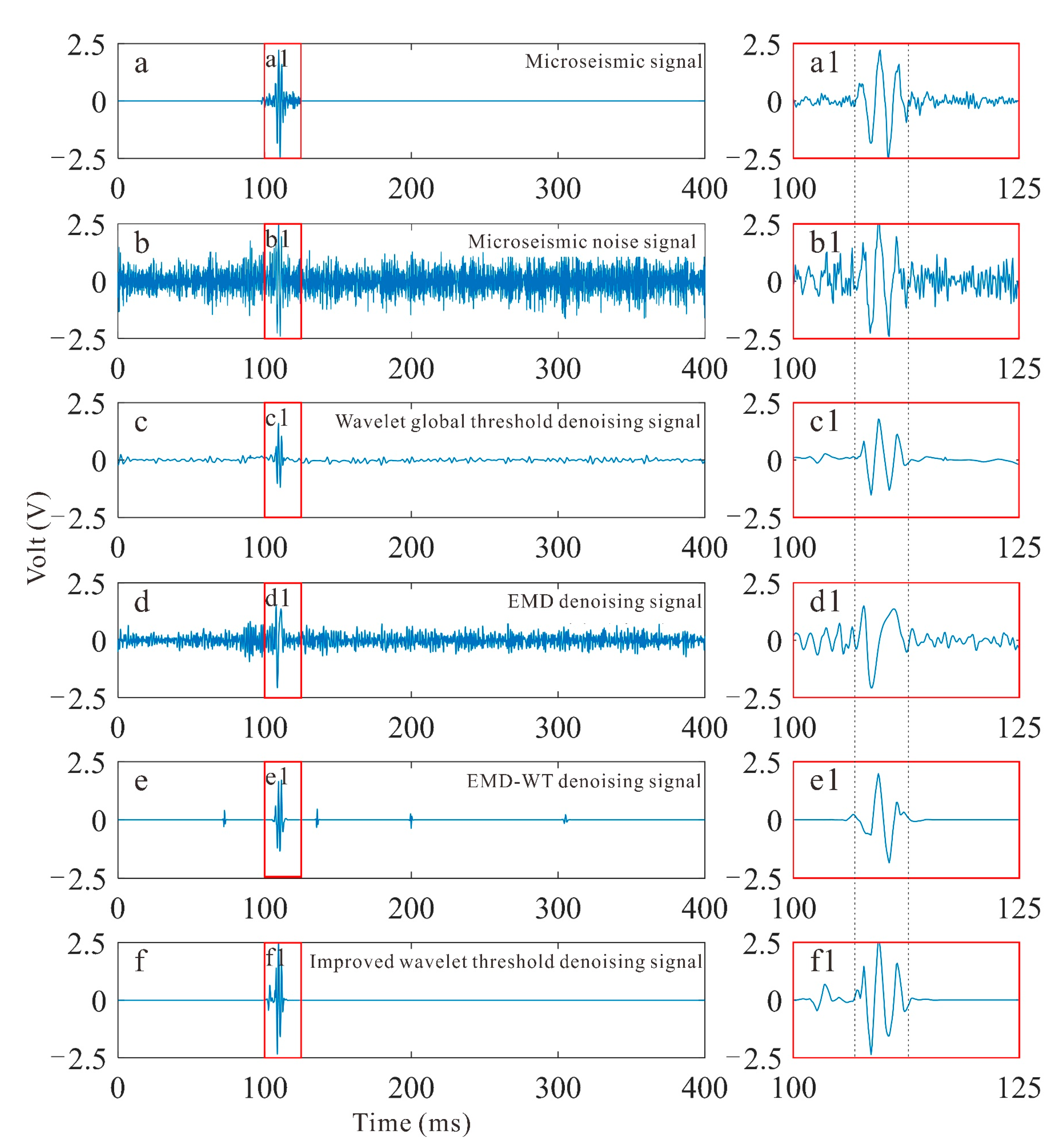
Figure 6.
Comparison of the denoising results of t different methods for microseismic current synthesis signals: (a,a1) microseismic signal, (b,b1) microseismic current signal, (c,c1) Wavelet global threshold denoising signal, (d,d1) EMD denoising signal, (e,e1) EMD-WT denoising signal, (f,f1) improved wavelet threshold denoising signal.

Figure 7.
Comparison of the denoising results of the microseismic noise current synthesis signal: (a,a1) microseismic signal, (b,b1) microseismic noise current signal, (c,c1) Wavelet global threshold denoising signal, (d,d1) EMD denoising signal, (e,e1) EMD-WT denoising signal, (f,f1) improved wavelet threshold denoising signal.
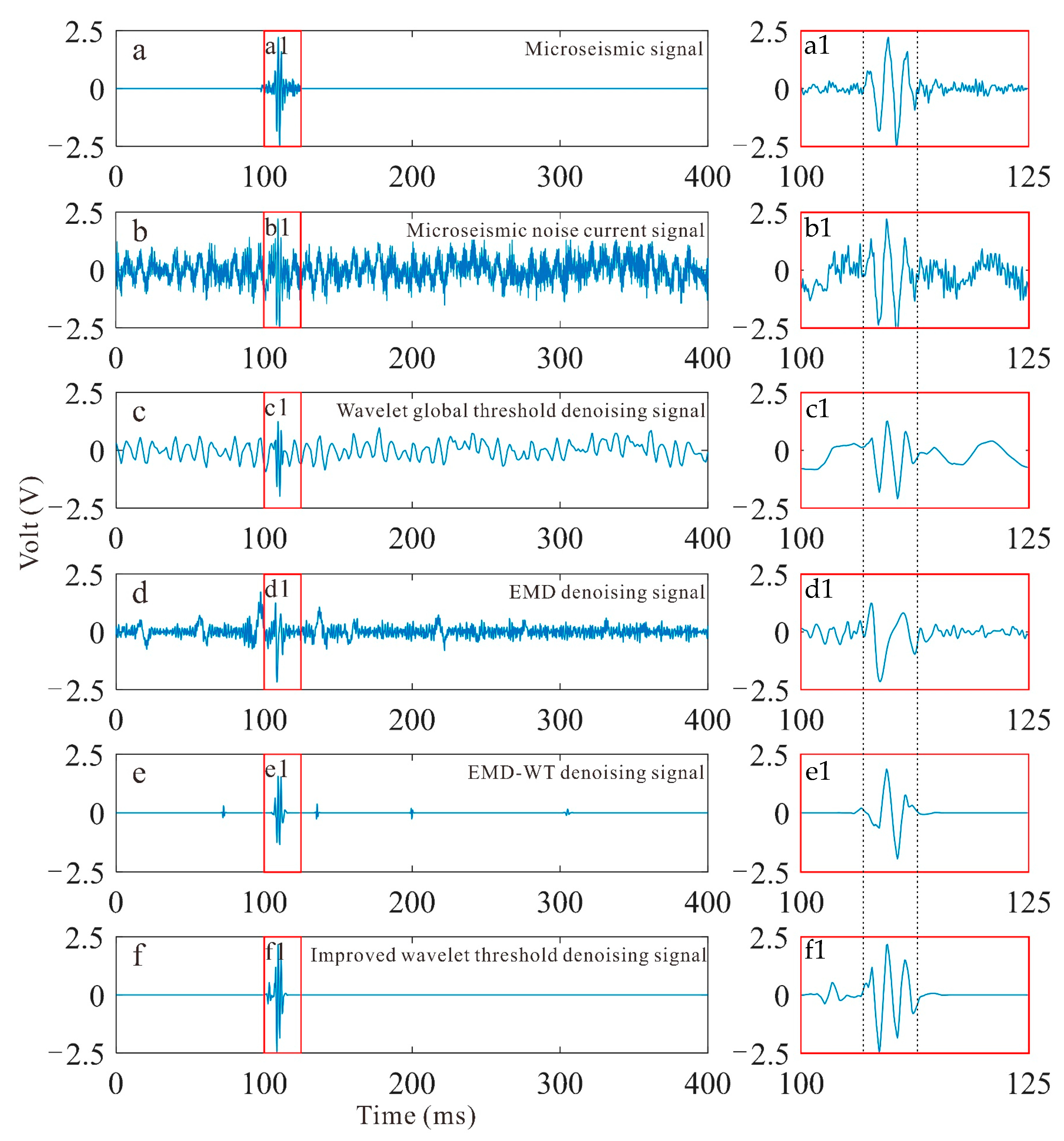
Figure 8.
Comparison of denoised synthesized microseismic signals with different SNRs: (a) microseismic noise of SNR = −10, (b) microseismic noise of SNR = −7, (c) microseismic noise of SNR = −4, (d) microseismic noise of SNR = −2, (a1,b1,c1,d1) Wavelet global threshold denoising signal, (a2,b2,c2,d2) EMD denoising signal, (a3,b3,c3,d3) EMD-WT denoising signal, (a4,b4,c4,d4) improved wavelet threshold denoising signal.
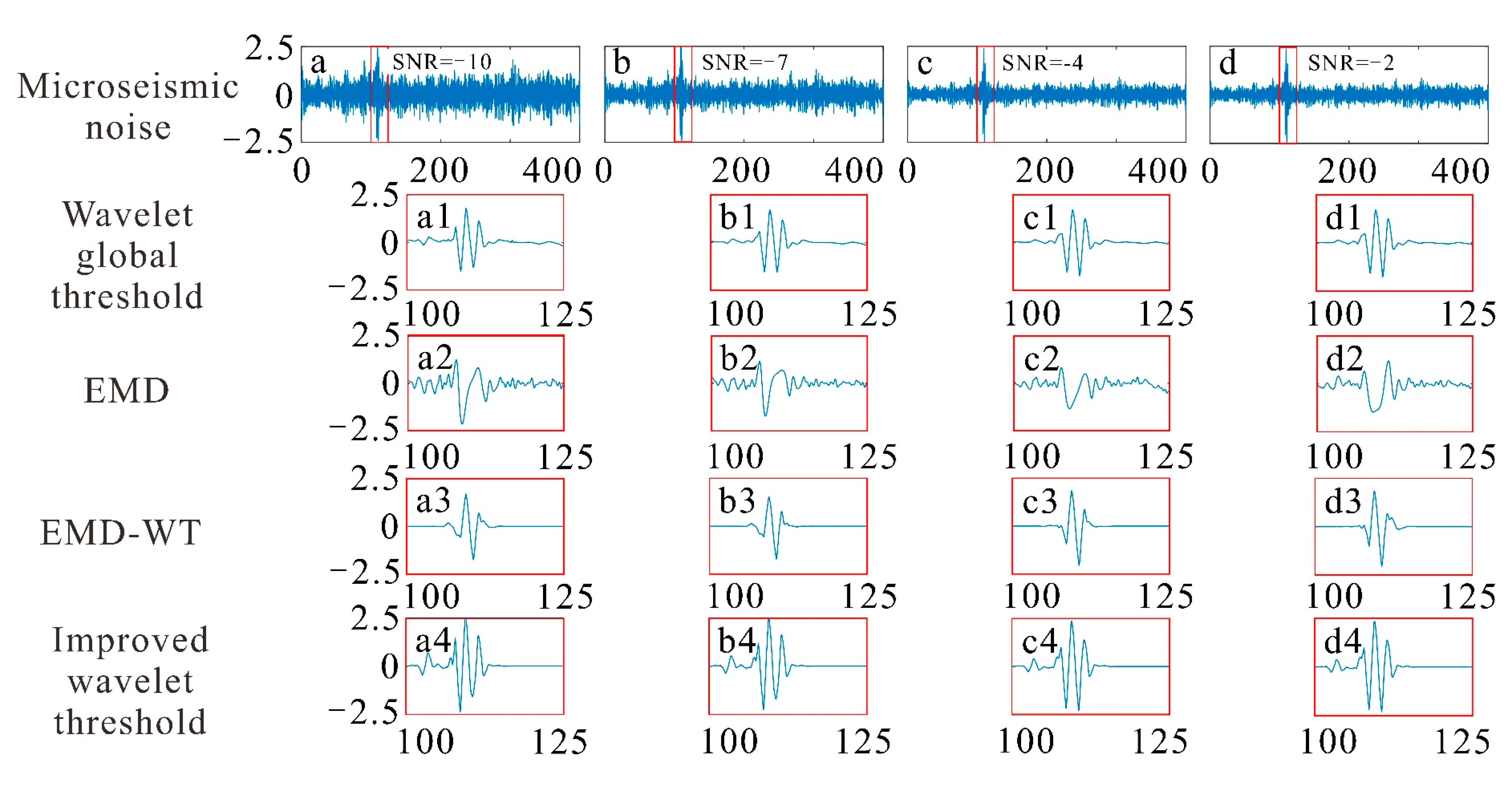
Figure 9.
Comparison of the denoising of synthesized microseismic current signals with different SNRs: (a) microseismic current of SNR = −10, (b) microseismic current of SNR = −7, (c) microseismic current of SNR = −4, (d) microseismic current noise of SNR = −2, (a1,b1,c1,d1) Wavelet global threshold denoising signal, (a2,b2,c2,d2) EMD denoising signal, (a3,b3,c3,d3) EMD-WT denoising signal, (a4,b4,c4,d4) improved wavelet threshold denoising signal.

Figure 10.
Comparison of the denoising of synthesized microseismic signals with noise, current and different SNRs: (a) microseismic noise current of SNR = −10, (b) microseismic noise current of SNR = −7, (c) microseismic noise current of SNR = −4, (d) microseismic noise current of SNR = −2, (a1,b1,c1,d1) Wavelet global threshold denoising signal, (a2,b2,c2,d2) EMD denoising signal, (a3,b3,c3,d3) EMD-WT denoising signal, (a4,b4,c4,d4) improved wavelet threshold denoising signal.
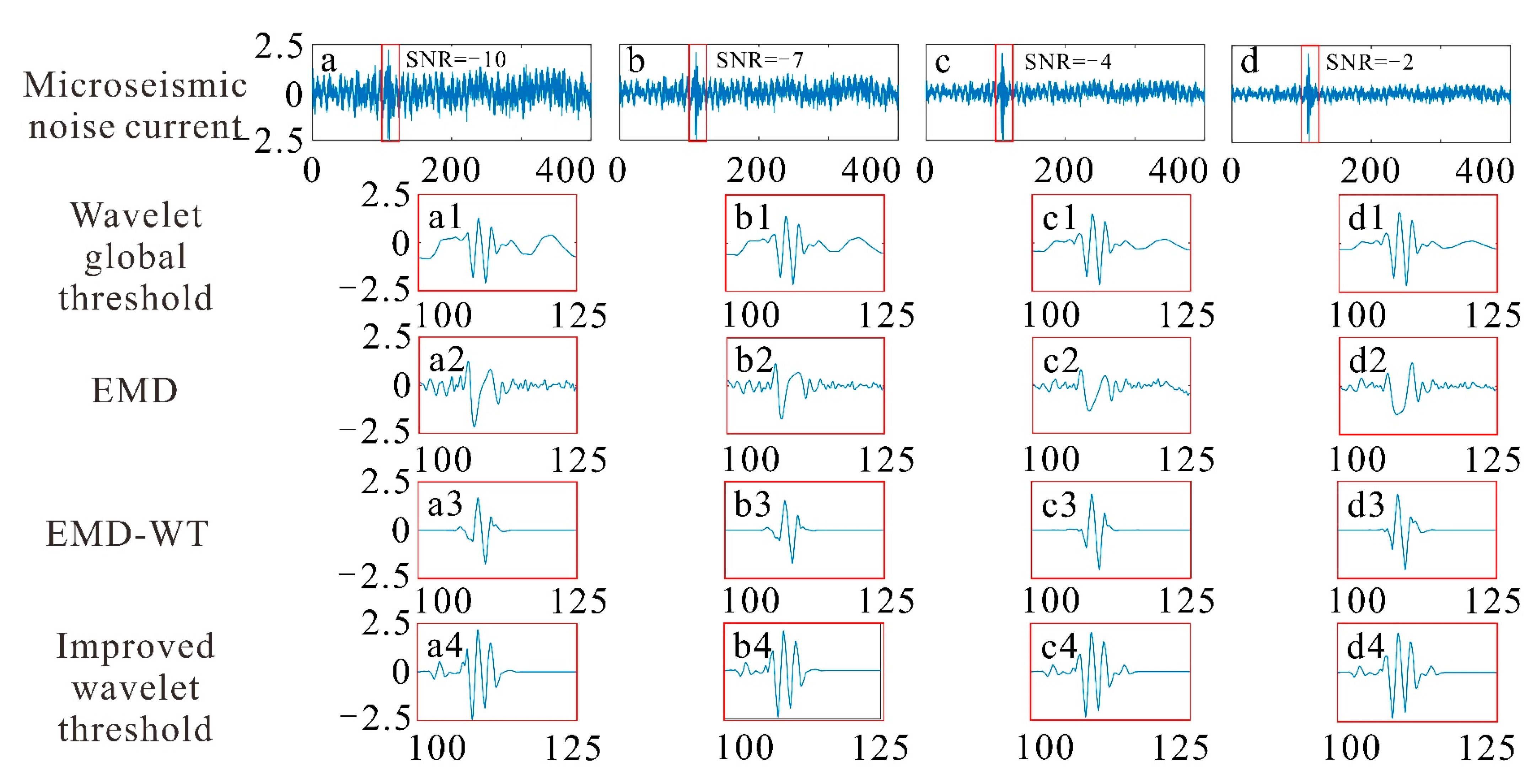
Figure 11.
Comparison of different synthetic signal evaluation indicators at different SNRs; (a) and (b) microseismic noise signal indicators, (c,d) microseismic current signal indicators and (e,f) microseismic noise current signal indicators.
Figure 11.
Comparison of different synthetic signal evaluation indicators at different SNRs; (a) and (b) microseismic noise signal indicators, (c,d) microseismic current signal indicators and (e,f) microseismic noise current signal indicators.
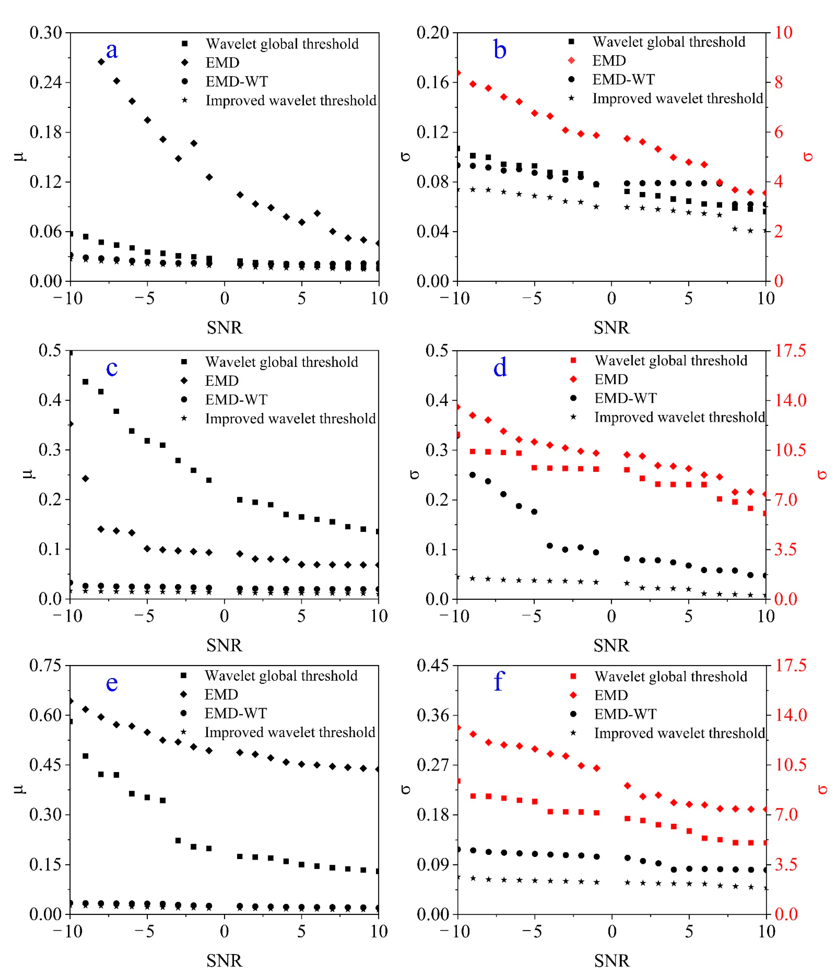
Figure 12.
Comparison of denoising effects for an actual microseismic noise signal: (a) microseismic noise signal, (b) Wavelet global threshold denoising signal, (c) EMD denoising signal, (d) EMD-WT denoising signal, (e) improved wavelet threshold denoising signal.
Figure 12.
Comparison of denoising effects for an actual microseismic noise signal: (a) microseismic noise signal, (b) Wavelet global threshold denoising signal, (c) EMD denoising signal, (d) EMD-WT denoising signal, (e) improved wavelet threshold denoising signal.
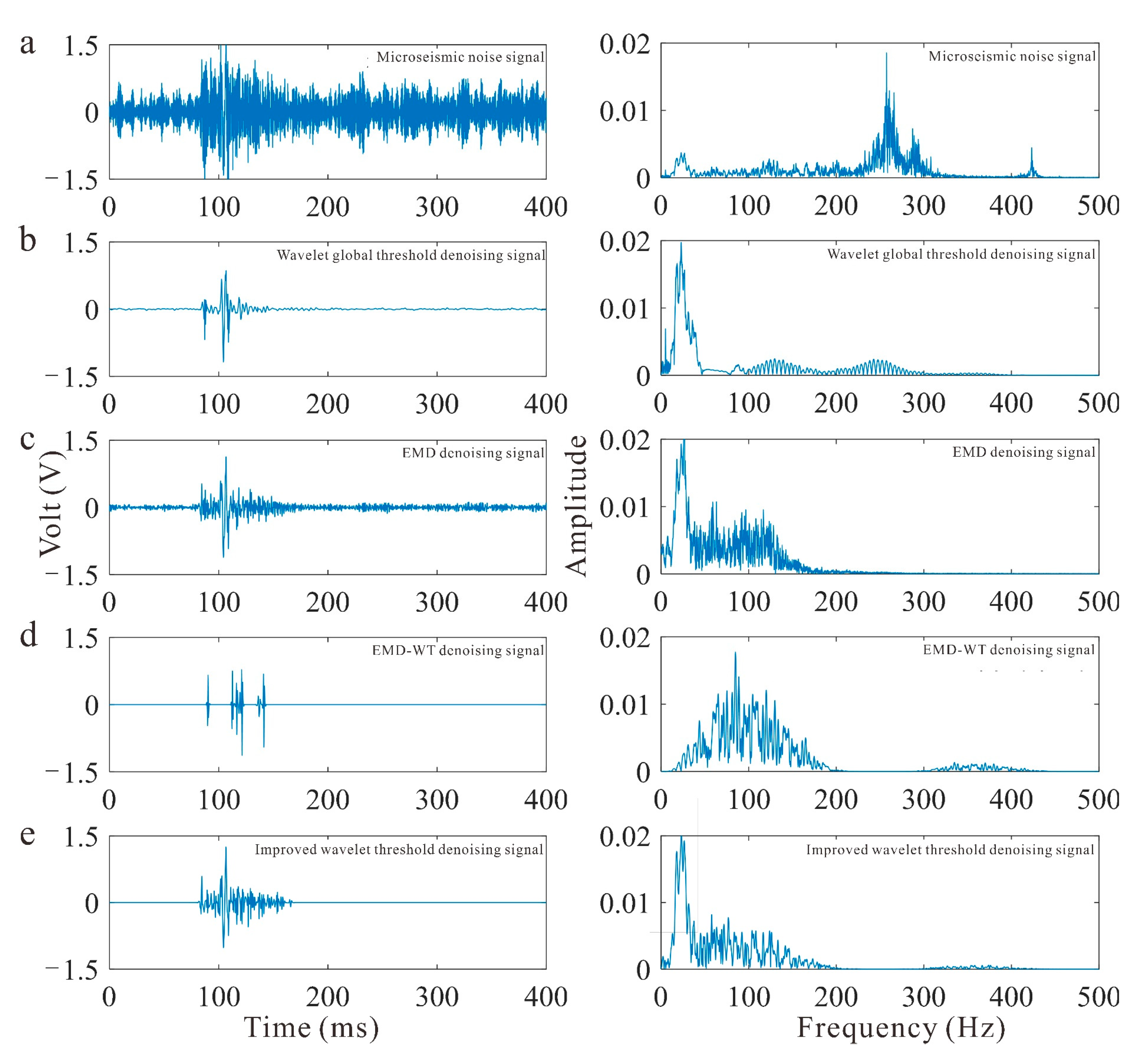
Figure 13.
Comparison of denoising effects for an actual microseismic current signal: (a) microseismic current signal, (b) Wavelet global threshold denoising signal, (c) EMD denoising signal, (d) EMD-WT denoising signal, (e) improved wavelet threshold denoising signal.
Figure 13.
Comparison of denoising effects for an actual microseismic current signal: (a) microseismic current signal, (b) Wavelet global threshold denoising signal, (c) EMD denoising signal, (d) EMD-WT denoising signal, (e) improved wavelet threshold denoising signal.
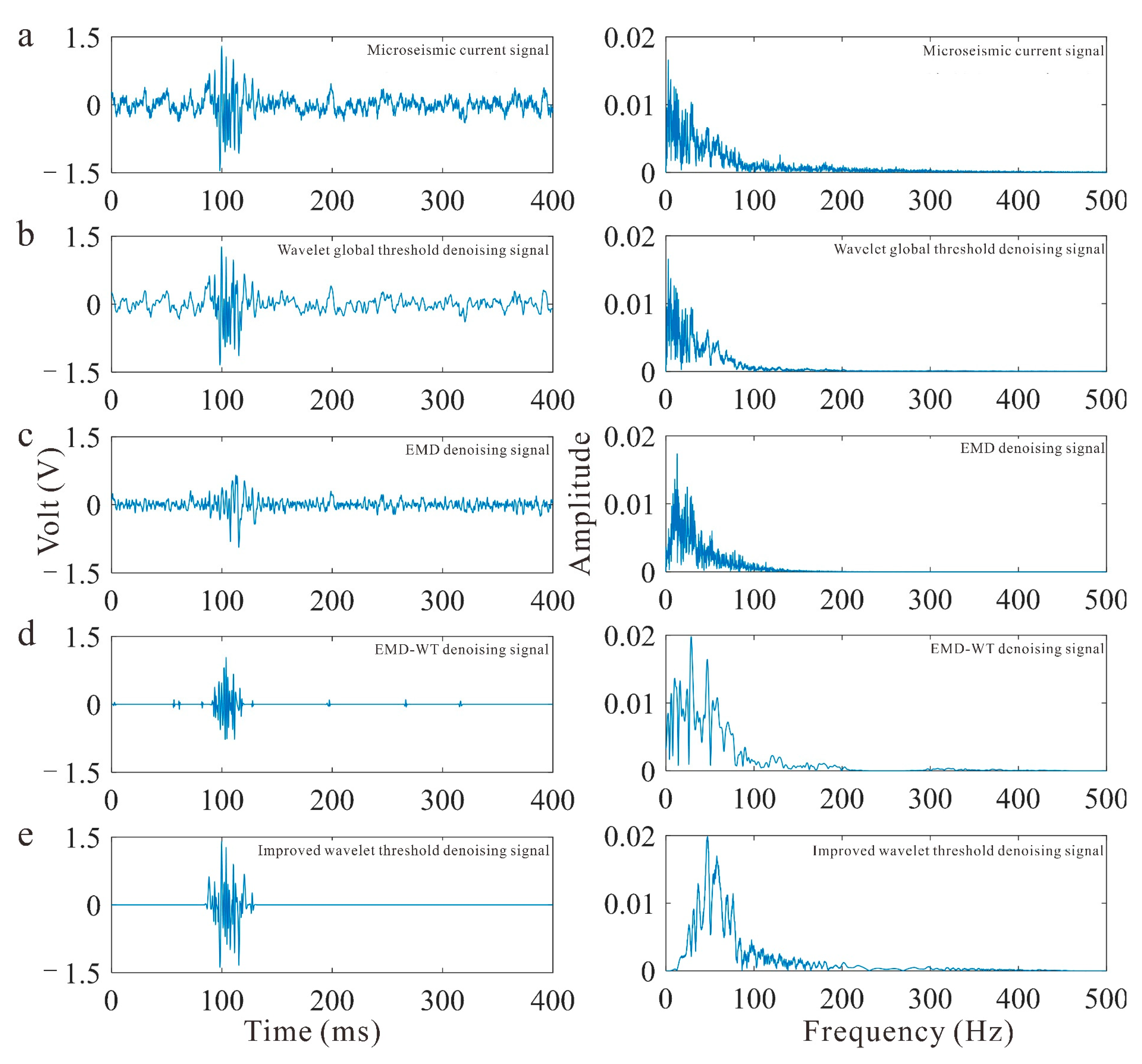
Figure 14.
Comparison of denoising effects for an actual microseismic signal with noise and current: (a) microseismic noise current signal, (b) Wavelet global threshold denoising signal, (c) EMD denoising signal, (d) EMD-WT denoising signal, (e) improved wavelet threshold denoising signal.
Figure 14.
Comparison of denoising effects for an actual microseismic signal with noise and current: (a) microseismic noise current signal, (b) Wavelet global threshold denoising signal, (c) EMD denoising signal, (d) EMD-WT denoising signal, (e) improved wavelet threshold denoising signal.

Figure 15.
Comparison of the SNR distributions for different types of microseismic data after denoising: (a) microseismic noise signal, (b) microseismic current signal and (c) microseismic signal with noise and current.
Figure 15.
Comparison of the SNR distributions for different types of microseismic data after denoising: (a) microseismic noise signal, (b) microseismic current signal and (c) microseismic signal with noise and current.

Table 1.
Comparison of decomposition layers.
| Decomposition Layers | μ | σ |
|---|---|---|
| 4 | 0.0237 | 0.0736 |
| 5 | 0.0346 | 0.0798 |
| 6 | 0.0482 | 0.0826 |
| 7 | 0.0688 | 0.0826 |
Table 2.
Comparison of the denoising effects of hard threshold, soft threshold and improved threshold functions for signals with different SNRs.
Table 2.
Comparison of the denoising effects of hard threshold, soft threshold and improved threshold functions for signals with different SNRs.
| SNR | Hard Threshold | Soft Threshold | Improved Threshold | |||
|---|---|---|---|---|---|---|
| μ | σ | μ | σ | μ | σ | |
| 5 | 0.0109 | 0.0879 | 0.0050 | 0.0544 | 0.0041 | 0.0348 |
| −2 | 0.0127 | 0.0946 | 0.0071 | 0.0602 | 0.0059 | 0.0566 |
| −10 | 0.0137 | 0.0994 | 0.0107 | 0.0745 | 0.0083 | 0.0622 |
Table 3.
Comparison of evaluation indicators for different types of synthetic signals.
| Synthesis Signal Types | Wavelet Global Threshold | EMD | EMD-WT g | Improved Wavelet Threshold | ||||
|---|---|---|---|---|---|---|---|---|
| μ | σ | μ | σ | μ | σ | μ | σ | |
| Microseismic noise | 0.4838 | 0.6842 | 0.2420 | 6.8444 | 0.0235 | 0.0892 | 0.0217 | 0.0736 |
| Microseismic current | 0.4953 | 0.6085 | 0.2522 | 6.3877 | 0.0237 | 0.1031 | 0.0166 | 0.0447 |
| Microseismic noise current | 0.4958 | 0.6534 | 0.2426 | 6.4657 | 0.0246 | 0.0890 | 0.0229 | 0.0791 |
Table 4.
The SNR MSE and r values after denoising based on an actual microseismic signal.
| Denoising Method | Evaluation Indicator | Noise Signal | ||
|---|---|---|---|---|
| Microseismic Noise | Microseismic Current | Microseismic Noise Current | ||
| Wavelet global threshold | SNR | 25.3288 | 5.9592 | 13.3623 |
| MSE | 0.0113 | 0.0180 | 0.0997 | |
| r | 0.5222 | 0.5789 | 0.4791 | |
| EMD | SNR | 10.1585 | 10.1868 | 8.2862 |
| MSE | 0.0313 | 0.0942 | 0.0850 | |
| r | 0.4036 | 0.7139 | 0.6695 | |
| EMD-WT | SNR | 31.4134 | 16.9703 | 30.1518 |
| MSE | 0.0019 | 0.0206 | 0.1634 | |
| r | 0.2681 | 0.3872 | 0.1210 | |
| Improved wavelet threshold | SNR | 47.9287 | 22.9659 | 39.3210 |
| MSE | 0.0011 | 0.0062 | 0.0547 | |
| r | 0.6923 | 0.9163 | 0.7924 | |
Disclaimer/Publisher’s Note: The statements, opinions and data contained in all publications are solely those of the individual author(s) and contributor(s) and not of MDPI and/or the editor(s). MDPI and/or the editor(s) disclaim responsibility for any injury to people or property resulting from any ideas, methods, instructions or products referred to in the content. |
© 2023 by the authors. Licensee MDPI, Basel, Switzerland. This article is an open access article distributed under the terms and conditions of the Creative Commons Attribution (CC BY) license (https://creativecommons.org/licenses/by/4.0/).
Share and Cite
MDPI and ACS Style
Tang, S.; Ding, S.; Li, J.; Zhu, C.; Cao, L. An Improved Microseismic Signal Denoising Method of Rock Failure for Deeply Buried Energy Exploration. Energies 2023, 16, 2274. https://doi.org/10.3390/en16052274
AMA Style
Tang S, Ding S, Li J, Zhu C, Cao L. An Improved Microseismic Signal Denoising Method of Rock Failure for Deeply Buried Energy Exploration. Energies. 2023; 16(5):2274. https://doi.org/10.3390/en16052274
Chicago/Turabian StyleTang, Shibin, Shun Ding, Jiaming Li, Chun Zhu, and Leyu Cao. 2023. "An Improved Microseismic Signal Denoising Method of Rock Failure for Deeply Buried Energy Exploration" Energies 16, no. 5: 2274. https://doi.org/10.3390/en16052274
Note that from the first issue of 2016, this journal uses article numbers instead of page numbers. See further details here.