
Uncertainty Quantification Analysis of Exhaust Gas Plume in a Crosswind


Dipartimento di Ingegneria Meccanica, Energetica, Gestionale e dei Trasporti (DIME), Università degli Studi di Genova, Via Montallegro 1, 16145 Genoa, Italy
*
Author to whom correspondence should be addressed.
Energies 2023, 16(8), 3549; https://doi.org/10.3390/en16083549
Submission received: 10 March 2023
/
Revised: 7 April 2023
/
Accepted: 17 April 2023
/
Published: 19 April 2023
Abstract
:The design of naval exhaust funnels has to take into account the interaction between the hot gases and topside structures, which usually includes critical electronic devices. Being able to predict the propagation trajectory, shape and temperature distribution of an exhaust gas plume is highly strategic in different industrial sectors. The propagation of a stack plume can be affected by different uncertainty factors, such as those related to the wind flow and gas flow conditions at the funnel exit. The constant growth of computational resources has allowed simulations to gain a key role in the early design phase. However, it is still difficult to model all the aspects of real physical problems in actual applications and, therefore, to completely rely upon the quantitative results of numerical simulations. One of the most important aspects is related to input variable uncertainty, which can significantly affect the simulation result. With this aim, the discipline of Uncertainty Quantification provides several methods to evaluate uncertainty propagation in numerical simulations. In this paper, UQ procedures are applied to a CFD simulation of a single plume in a crossflow. The authors test the influence of the uncertainty propagation of the chimney exit velocity and the main flow angle on the plume flow development. Two different UQ methods are applied to the analysis: the surrogate-based approach and the polynomial chaos expansion method. A comparison of the two methods is performed in order to find their pros and cons, focusing on the different and detailed quantities of interest.
1. Introduction
In the ship design practice, short funnels and tall masts are usually created, where electronic devices (radars, antennas, etc.) are housed. This aspect can generate problems with hot exhaust gases, which can be trapped on the ship deckhouse, exposing these areas to high temperatures that can seriously affect ventilation, passengers’ comfort or electronic systems failure; for a military vessel, it can cause problems to the weapon systems and increase the infrared signature. Nowadays, the use of gas turbines as the main marine propulsion system has exacerbated this problem compared to diesel engines due to an increase in the exhaust gas mass flow rate and temperature. For all the above reasons, it is crucial to accurately predict the temperature patterns in the exhaust plume. Baham and McCallum [1] have performed full-scale measurements of exhaust plume temperatures in a warship, suggesting a step-by-step procedure for estimating the downwind plume gas temperature and trajectories. Kulkami et al. [2] studied the evolution of the ship funnel over the last hundred years, the present state of modern warship funnels vis-à-vis the location of superstructures along with various electronics and provided a review of various studies from the 1930s.
Similar to the exhaust plume problem, many researchers in other fields have numerically and experimentally studied a single round heated jet normally injected into a crossflow. Starting from the 1950s, Morton et al. [3] investigated the spread of a turbulent buoyant jet from a source. This article is the basis for the development of several plume integral models, all based on conservation equations of mass, momentum and energy, with empirical coefficients added and some simplifications to describe the interaction between the plume and the environment (the entrainment effect). The work by Slawson and Csanady [4] considered first the effect of the atmosphere on the plume’s rise with a simplified model. Subsequently, several other authors have updated the above model [5,6,7,8]. Muldoon et al. [9] performed a DNS of a plume, while simpler applications with RANS equations and commercial software have been developed to be routinely used. Hargreaves et al. [10] developed a simplified simulation of a plume development: in this analysis, the authors substituted the stack with energy and momentum sources, which generate the plume. König et al. [11] used a numerical approach in order to compare different chimney exit configurations. Mahjoub Saïd et al. [12] conducted a very detailed analysis on the flow field of a plume in a crossflow: they compared the numerical simulation results with the PIV experimental measurements.
In the last decade, several studies have been conducted on the plumes or jets for different sectors. Shah et al. [13] performed a numerical study for a sonic jet from a blunted cone to provide possible directional control in a supersonic crossflow by solving the unsteady Reynolds-averaged Navier–Stokes (RANS) equations. Xing et al. [14] presented a reduced-scale field experiment to model a CO2 blowout for the purpose of acquiring concentration distribution in the flow field; a CFD code was used to analyze the interior structure of the CO2 plume. Oliveira et al. [15] numerically simulated an MDI spray plume by considering the spray droplets and evaporation. Jatale et al. [16] performed an LES of a helium plume, validating it through experimental measures from Sandia National Laboratory. Olsen and Skjetne [17] simulated the underwater bubble plumes emerging from a subsea release of gas to demonstrate that the choice of mass transfer coefficient strongly affects the amount of gas dispersion. Brusca et al. [18] developed a Gaussian plume mathematical model to study the emission of particulate matter by varying the wind velocity and PM mass flow rate. Toja-Silva et al. [19] presented a CFD model of carbon dioxide dispersion from a natural-gas-fueled thermal power plant in an urban environment; the characteristics of the CO2 plume were analyzed by comparing it with a Gaussian plume model. Tominaga and Stathopoulos [20] simulated the flow dispersion around an isolated cubic building model with tracer gases released from an exit behind the building with different buoyancy models. Wang et al. [21] investigated, with a very simple scaled model, the starting plume rising from a mountain due to the transient natural convection of the sun’s radiation; the importance of the thermal boundary layer was underlined for the transient flows. Granados-Ortiz et al. [22] studied the influence of both experimental and parametric uncertainty from the turbulence intensity in the computation of an under-expanded jet flow. Sedighi and Bazargan [23] investigated the mixing and merging of buoyant exhaust plumes originating from multiple small cooling towers in the atmosphere, focusing on the counter-rotating vortex pair as the dominant mechanism affecting the flow pattern. Bai et al. [24] used an existing meteorological model to study SO2 diffusion from a single ship. Baum and Gibbes [25] investigated near-field brine discharge dynamics for a desalination plant offshore; different longshore crossflow conditions were examined to quantify the impact distance, dilution and terminal rise. Liu et al. [26] experimentally studied the evolution of the fire plume centerline temperature for risk analysis by revealing the effects of the ullage height. Dewar et al. [27] developed a new multi-phase leakage plume model integrated with coastal hydrodynamics to predict CO2 and pH. Wang et al. [28] combined a CFD code with the Dijkstra algorithm to simulate toxic gas dispersion to calculate the optimal route with the minimal total inhaled dose by varying the wind direction. Zhang et al. [29] studied a bubbly jet crossflow to explore the hydrodynamics using OpenFOAM; the effects of ambient crossflow on bubbly jet behaviors were systematically examined. Hu et al. [30] studied offshore ship emissions in port cities through a drone model.
The experience gained by the authors on ship exhaust fumes propagation has confirmed how much the trajectory and shape of a chimney plume can be affected by the uncertainties of external (wind flow characteristics) and internal (exhaust gas fluid dynamics characteristics at the chimney exit) parameters. The use of Uncertainty Quantification can support the understanding of physical problems. A single plume in a crossflow case is considered in the present analysis in order to demonstrate the use of UQ techniques for the specific problem and its potential for more complex cases, such as fume evolution on a ship deckhouse. The use of Uncertainty Quantification (UQ), to improve the accuracy and reliability of numerical simulations, is increasingly effective in many engineering fields for industrial applications thanks to recent improvements in both soft-computing algorithms and hardware performance [31,32,33,34]. With the use of the UQ techniques, it can be quantified how uncertainty propagates through the physical problems and how it can affect the simulation results. Computational fluid dynamics (CFD) is one of the latest disciplines where UQ techniques have been exploited with increasing relevance. The recent developments in response surface methodology (RSM), which is normally very effective for optimization in design processes [35,36], have also led the way for the application of UQ to this field [37,38,39]. Several UQ methods have been applied in stochastic fluid dynamics problems, including Monte Carlo (MC—whose accuracy is affected by the sampling point number), perturbation method, moment method and surrogated models. The latter has been developed in order to investigate uncertainty propagation problems, such as polynomial chaos expansion (PCE) [40,41,42,43], low-rank tensor approximations [44], Gaussian process modeling [45], the radial basis function (RBF) [46], machine learning methods (using artificial neural networks (ANNs) [47]) and deep learning models [48]. Xia et al. [49] introduced a non-intrusive polynomial chaos method (NIPC) to quantify the uncertainty of resistance, sinkage and trim of the Japan Bulk Carrier model advancing with an uncertain speed in shallow water; the NIPC was compared to the MC, showing its higher efficiency in UQ.
This research group’s interest in fluid dynamics modeling of turbulent flows in industrial or environmental applications [50,51,52,53] has motivated the authors to test UQ methodologies in the CFD simulation of a 3D plume, starting from a cylindrical chimney and subject to a crossflow, which is a relevant case for all the practical applications listed above. The main target of this paper is to demonstrate the use of UQ methods in the CFD simulation of a plume in a crossflow in order to evaluate how uncertainties from the input variables can affect the uncertainty of the results. The selected input variables are the exit velocity of the fumes, vf, and the crossflow angle, α.
Two different methods for uncertainty propagation are introduced using an automated procedure into an open-source software platform (Dakota [54,55]): the surrogate-based approach (SB) and the polynomial chaos expansions (PCEs). The former is based on the construction of a Design of Experiments (DoE) to represent the model response to the variation in a defined set of input variables within a certain design space. The values of the input variables are selected through a random sampling algorithm, the Latin hypercube sampling (LHS) method. From the validated DoE (simulation of the full set using 3D CFD), the surrogate model is generated through a Gaussian process approach. The UQ analysis, based on hundreds of samples, can be efficiently performed, with limited computational cost, thanks to the use of the meta-model instead of the “physical model” (3D CFD simulations). The latter approach is based on a multidimensional orthogonal polynomial chaos approximation (PCE) formed with standardized random variables. In Dakota, the PCE approach uses the Wiener–Askey scheme with different polynomials for modeling the different probability distributions (e.g., Hermite polynomials for normal pdf and Legendre polynomials for uniform pdf) [54,55]. Both methods are applied to the plume problem in order to discuss the advantages and disadvantages.
The scope of this work is to set up an effective and efficient UQ approach for the plume identification and evolution analysis that will be the reference procedure to use in practical applications, such as ship deck layout designs (subject to the propulsion system exhaust gases) or environmental problems related to plume evolution from industrial processes.
2. Numerical Model
2.1. Governing Equations
The physical–mathematical problem is set by the Reynolds-averaged Navier–Stokes equations. The conservation of mass and momentum are written in the Eulerian conservative divergence form:
where τ is the tensor of the normal and tangential stress due to viscosity, and SM is the momentum source. The turbulence closure adopted to model the momentum source (the Reynolds stress tensor) is the standard, k–ε [56,57]. This model has been applied to different industrial fluid dynamics applications [58,59]. The additional transport equations of the model are:
In these equations, Gk represents the generation of turbulent kinetic energy due to the mean velocity gradients; Gb is the generation of turbulent kinetic energy due to buoyancy; YM represents the contribution of the fluctuating dilatation in compressible turbulence to the overall dissipation rate; and Sk and Sε are source terms. The turbulent (or eddy) viscosity, µt, is computed by combining k and ε:
All the model coefficients are set in accordance with Ansys CFX, the commercial software adopted for the following numerical setup [60].
Finally, the resolutions of the energy equation in the fluid domain can be calculated with the following equation:
where the total enthalpy is equal to:
2.2. CFD Model
In order to simulate the plume and apply the UQ techniques, a chimney with a circular section of 10 [mm] and a height of 76 [mm] was considered. The external domain and chimney geometric characteristics are very close to that proposed by Mahjoub Saïd et al. [12] to be used for the CFD model validation. In particular, the chimney is located at 200 [mm] from the inlet and at 250 [mm] from the outlet, while the external computational domain has a parallelepiped shape with a lateral length of 450 [mm] and a height of 250 [mm] from the ground. All the geometrical characteristics of the fluid domain considered in this study are reported in Figure 1. A realistic order of magnitude for the scaling factor between the model and the prototype could be 1:100. However, the scaling factor can be different according to the application: in naval engineering, the exhaust funnel exit diameter varies due to the size and type of the engine (diesel, gas turbine, propulsion, generator, etc.) from less than 1 [m] to few meters.
The computational domain was discretized with a multiblock structured hexahedral grid with Ansys ICEM CFD 14.0 software. An O-grid block was generated around the chimney; the size of the O-grid block extends within a radius of almost 130 [mm] around the center of the funnel and has a variable cell size from almost 0.1 to 5 [mm]. In fact, near the walls, a minimum cell size was used to guarantee a Y+ of about 30 in order to activate the wall function modeling; a cell growth rate of 1.1 was adopted to de-refine the mesh toward the external boundaries. Cross blocks were generated in order to optimally control the distribution of the nodes. In the vertical direction, a uniform cell distribution was used. This grid was set up and selected after a sensitivity analysis in order to have negligible variation in the velocity profiles in a set of control stations. In Figure 2, a mesh cut plane in a vertical mid plane and a top surface mesh are reported.
The CFD software used for the simulations and post-processing was ANSYS CFX. The turbulence closure model chosen is the standard k–ε, which offers good results with stronger numerical stability for turbulent exhaust plumes [61,62]. The total energy option to solve the energy equation with respect to enthalpy was activated. The fluid modeled is air, treated as a perfect gas. The following boundary conditions were imposed: at the inlet of the external domain, the velocity and its direction (without atmospheric boundary layer), a uniform static temperature of 300 [K] and a uniform turbulence intensity equal to 5% were set for the crossflow. Uniform velocity and static temperature (600 [K]) with a medium turbulence intensity were fixed at the chimney exit. The opening condition with the ambient reference was set for the surfaces of the external domain; the chimney and ground surfaces were modeled as adiabatic walls with no-slip conditions. The same values used in [12] were fixed as boundary conditions. Finally, all the equations were solved for steady flow and with second-order numerical schemes.
2.3. Validation
For validation purposes, the reference control sections in Figure 3 were used.
In Figure 4, a comparison of the flow velocity components in the x and z directions, for the first control section, is reported. The results are generally in good agreement except for the peak, which is slightly underestimated for U (x-component) and overestimated for W (z-component).
The results for U velocity at the x = 16.7 [mm] section (Figure 5a) are very close to the experimental data, whereas the W component (Figure 5b) is far from the reference data. The authors of the reference paper discussed this problem and concluded that the measurements could have had large inaccuracy because the section had been placed in the wake region where the velocity modules are very small and give large measuring errors. Additionally, the Reynolds tensor components u’u’ and w’w’ were calculated and compared to the experimental data. The charts in Figure 6 compare the data for the second control section at x = 16.7 [mm], showing a good match of the numerical results with the experimental data. With the above validation, the CFD model is considered adequate for the plume characterization and for its systematic use in the UQ analysis.
3. Uncertainty Quantification Models
3.1. Surrogate-Based Sampling Method
This type of approach involves the use of a procedure marked by several fundamental phases. The first phase consists of building the DoE through a sampling technique such as the Monte Carlo (MC) method or the Latin Hypercube (LHS) method. The sampling of the input variables considered is obtained within the predetermined variation ranges. Through an automated procedure, the simulations are carried out with the sampled input parameters, and for each simulation, the results of the Quantities of Interest (QoI), i.e., the response quantities of the system, are reported. Once the DoEs for the response variables are obtained, the meta-model or surrogate model is built based on the validated DoE. Among the possible techniques that can be exploited, one of the most used is the Gaussian process method. The response surface approximated using the GP can be represented through the following expression [54,55]:
where represents the current point in a parametric space of n dimensions; is the vector of the basic trend functions calculated for ; is the vector containing the estimate of the quadratic deviations in the coefficients of the functions; is the correlation vector of the terms between and the points of the DoE; is the correlation matrix for all points; is the response vector; and is the matrix containing the trend functions evaluated at all points. A Gaussian correlation function is used to calculate the terms in the correlation vector and matrix, and the correlation parameters are obtained using a procedure called maximum likelihood estimation (MLE) [54,55].
3.2. Polynomial Chaos Expansion Method
The approximation is based on orthogonal polynomials, known as the Wiener–Askey scheme, which determines an optimal basis for multiple continuous probability distributions. The set of polynomials is used as an orthogonal basis to approximate the functionality between the stochastic response and each of the random inputs. The expansions for an answer, R, take the form [54,55]:
where are the deterministic coefficients to be calculated, are the orthogonal basis of polynomials and ξ is the vector of independent random variables. In our case, the expansion is approximated to a finite number of variables (the input variables) and to a finite expansion order so:
The PCE method allows for evaluating the model in a “strategic” way (through sampling, quadrature rule…) in order to evaluate , the coefficients of the orthogonal polynomial approximation of the response. The quadrature method is very efficient if the number of stochastic input variables is small. On the contrary, when the number of input variables is considerable, the approach runs into the phenomenon defined as the curse of dimensionality [54,55], which causes an exponential increase in the number of simulations required, making it not attractive with respect to the surrogate-based approach.
4. UQ Analysis: Uncertainty on Exhaust Gas Outlet Velocity vf
4.1. Sensitivity Analysis of vf
One of the most important parameters, which determines the plume evolution, is the velocity ratio, R, between the velocity magnitude at the chimney exit (vf) and the crossflow velocity (V):
The R variation has major effects on plume development, implying the change in both plume height and trajectory. The variation in vf was analyzed. Five simulations were performed with vf changed in the range of 16–24 [m/s], a resolution of 2 [m/s] and a fixed crossflow velocity equal to 8.0 [m/s]. The effect of the parameter is shown in Figure 7. In this picture, the contour maps of the plume temperature (this identifies the plume area) in a cross-section seen from the front (view from the incoming wind) are compared: as the vf increases, the height of the plume and the area of the map increase. In this view, there is symmetry with the chimney axis, and the flow structure has two counter-rotating vortices that dominate these contour maps.
To proceed with UQ analysis, the Quantities of Interest (QoI) have to be defined in order to characterize the plume flow changes with the input variable variations. A set of four control points (whose position with respect to the funnel center is reported in Table 1) and five control surfaces were placed behind the chimney in a section 30 [mm] from the axis, as shown in Figure 8a,b. Using the points as temperature probes and storing the maximum temperature on the surfaces, the trajectory changes in the plume can be detected and quantified. Moreover, the variation in the plume area on this surface is computed and stored (Figure 8c) in order to quantify the plume cross-section variation.
4.2. UQ Analysis of vf: Surrogate-Based Approach
The procedure consists of the creation of a DoE for the system response in the range of input variable variations. A DoE of 64 conditions was built and simulated using the above CFD model. The obtained variations for certain QoI are reported in Figure 9, Figure 10 and Figure 11. Only the output variables that showed a significant variation in the established range were considered.
Starting from the DoE values, the response functions (surrogate models) for the above QoI were obtained using the Gaussian process method. The UQ analysis is performed with LHS sampling on the above meta-models using 500 samples.
At first, a uniform distribution of the variable, vf (see Figure 12), in the range of 15–25 [m/s] was considered. The histograms depicted in Figure 13, Figure 14 and Figure 15 show the uncertainty distribution of the QoI. It can be noticed that the trend of the histograms is always different from the uniform input distribution. Only the cross-section area of the plume has a uniform uncertainty distribution (Figure 11), which testifies to a linear relationship with the input. Moreover, the variations in QoIs are not negligible, especially if compared to the uncertainty level of the input variable.
These results confirm the hypothesis that a relatively small change in the vf can cause a significant change in the QoI and, consequently, in the plume evolution.
A more representative analysis is performed with the introduction of a normal probability density function (pdf) for the input variables, which can more realistically simulate the uncertainty related to the gas velocity found at the exit of an exhaust funnel. An example is shown in Figure 16: it has a mean value centered in the range of (20 [m/s]) with a standard deviation of 2 [m/s], which is the estimated uncertainty of the variable, selected from the experience of previous works [37,38,39]; the aim is to verify the effect of a small deviation from the mean.
The above uncertainty propagation through the model leads to the output QoI distributions shown in Figure 17, Figure 18 and Figure 19. As in the previous analysis, the probability distribution of the output QoI is, in general, different from a Gaussian trend except for the area. This means that, given a normal input velocity distribution, the resulting output pdfs are non-symmetrical with respect to the mean value, with a shift in more probable values to higher temperatures (see Tmax,1 in Figure 18) or to ambient conditions (see Tpoint,4 in Figure 17). For the plume area, on the other hand, an almost linear correlation between the QoI and the vf makes the pdf similar to a normal distribution; this leads to an immediate prediction of the surface that can be affected by the highest temperature values and gradients. The uncertainty propagation is quantified by the values of standard deviation, σ, in the output pdf reported in Table 2. Compared to a σ value of 10% with respect to the mean, the uncertainty obtained for the output can be relevant.
4.3. UQ Analysis of vf: Polynomial Chaos Approach
The PCE method has a great positive impact on UQ problems where the number of input variables subjected to uncertainty is less than five [54,55]. In these cases, the analysis can be performed with a limited number of simulations to build the meta-model based on polynomial approximation. For this reason, the PCE can be a valid alternative method to perform an analysis of the plume in a crossflow. Only 16D CFD calculations were carried out to build the PCE method, instead of 64 CFD simulations, as in the previous method. The results for a selection of QoI obtained using a normal pdf for the input variable, vf, are shown in Figure 20. In the figure, the results are compared to those of the meta-model-based approach.
The comparison for the distributions obtained with the PCE method highlights a very good match with the results from the surrogate-based approach. The PCE method has a significantly reduced computational cost for the UQ analysis with the same output as the more expensive surrogate method.
5. UQ Analysis: Uncertainty on Incoming Wind Angle α
5.1. Sensitivity Analysis of Wind Direction α
As for the exit velocity, a set of simulations were performed varying the wind angle for a preliminary sensitivity analysis, which is useful to identify the input variable range and to check the system response to different values of this input parameter. With a fixed velocity ratio R = 2.0, the α is varied in the range [0.0,10.0] with 2.0 deg of resolution; this is the wind angle in the horizontal plane with respect to a normal crossflow (as seen in Figure 1). The effect of the flow angle variation on the plume flow structure is shown in Figure 21, where the contour maps of temperature are drawn in a plume cross-section seen from the front (view from the domain inlet).
The effect of α generates a shift in the plume and its flow structure with the counter-rotating vortices according to the main flow direction and does not significantly affect the shape and the surface dimension of the plume cross-section.
5.2. UQ Analysis of α: Surrogate-Based Approach
In order to evaluate the influence of the uncertainty related to this parameter, a UQ analysis was performed in the range explored in the previous section. The QoI recorded are the temperatures in points 1-5-6-7, as depicted in Figure 8. The DoE is made of 64 simulations, and the results are shown in Figure 22.
Figure 23 shows the pdf histograms for the QoI with a Gaussian distribution of the input variable, α, in the range [0.0,10.0] degree, with a mean value of 5 degrees and a standard deviation of 1 degree (see Figure 24).
The mean and standard deviation in the output distributions can be obtained and are reported in Table 3.
The uncertainty of the temperature can be considered almost negligible, considering that the σ of the input variable is 20% of the mean value.
5.3. UQ Analysis of α: Polynomial Chaos Approach
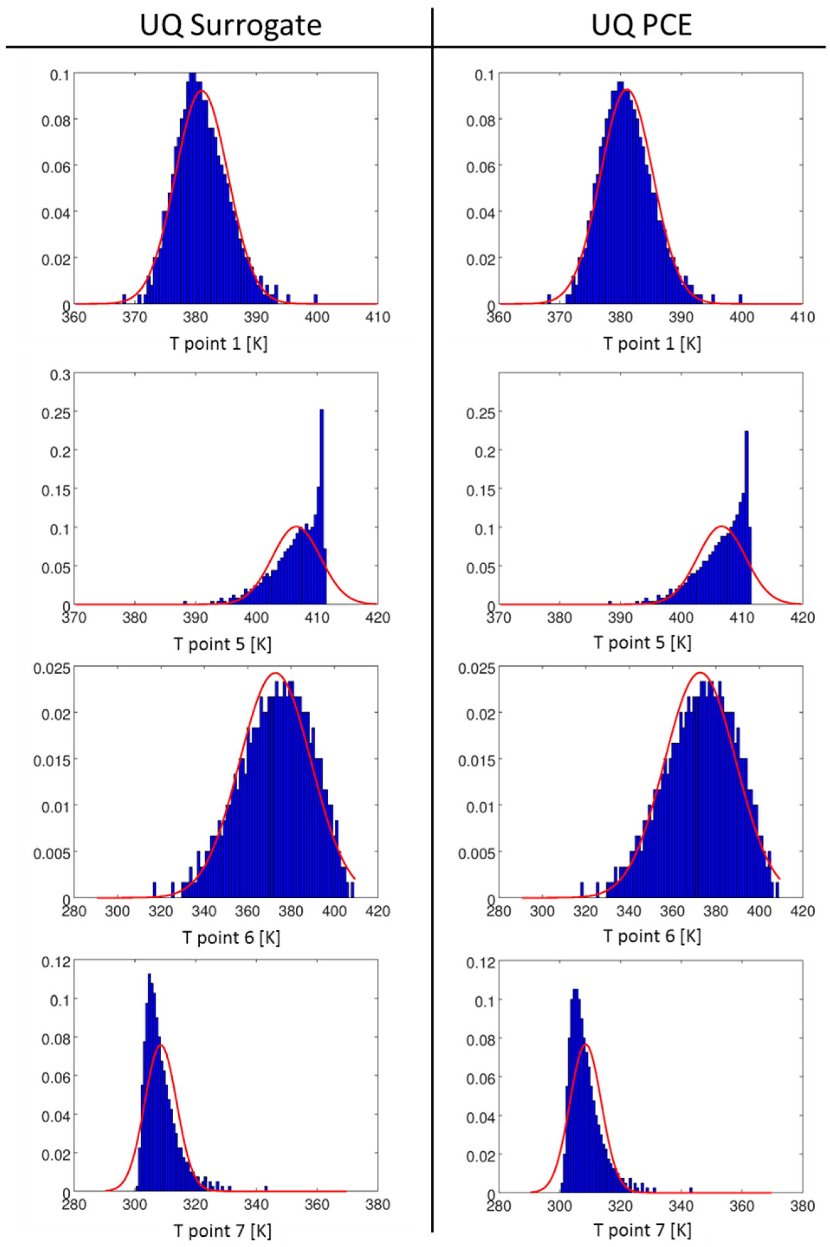
To complete the set of analyses, the PCE approach was tested also for this case. Only six calculations were performed to set the polynomial chaos method. The obtained results from the same analysis performed using the surrogate models are very similar to those obtained with the surrogate-based approach, as shown in Figure 25.
6. Conclusions
A plume in a crossflow is a reference case study for many practical applications in industrial and environmental flows, and the experience gained with the above research activity, together with the UQ software platform setup, is a precious background for the setup of more articulate applications in practical cases. The results from this work can be useful as a first reference for plume evolution in a large variety of situations for industrial and environmental applications.
In this paper, an original method for plume identification was presented, and a set of QoI was introduced to understand and quantify the effects of uncertainties for the input variables (vf and α) on the evolution of a plume in a crossflow. As a general outcome, it was highlighted that the variation in the exit fume velocity (velocity ratio R) has a significant impact on the plume flow structure, while the uncertainties of the incoming wind flow angle, α, are much less important. It was verified that even with a uniform uncertainty distribution, the outputs obtained from the UQ analysis show a relevant asymmetry and non-uniformity due to the strong non-linearity of the physical problem. The above results were obtained with both surrogate-based and polynomial-chaos-based UQ methods. The limited computational efforts needed to set up the PCE method make this approach very attractive for industrial applications where a limited number of input variables affected by uncertainty is considered. The simulation model coupled with the UQ techniques presented in this paper demonstrates the need for this kind of analysis to reduce the risk of a weak design solution or wrong conclusions when the most relevant input parameters are uncertain. The exhaust plume evolution problem is certainly part of the above situations; the results are frequently crucial in critical industrial or environmental problems, especially when legal aspects may be involved. The effects of uncertainty could support the evidence or not, from guilt or innocence.
Author Contributions
C.C., D.D.D. and D.M. equally contributed to the concept of the research activity, the setup of the model, the discussion of the results and the writing of the paper. All authors have read and agreed to the published version of the manuscript.
Funding
This research activity has been funded by the company CETENA Spa from Fincantieri Group whose support is warmly acknowledged. The research team from the University of Genova is grateful to the technical group of CETENA for their support in the discussion of the complex topics involved and for the great occasion offered to work on this very specific application.
Data Availability Statement
Not applicable.
Conflicts of Interest
The authors declare no conflict of interest.
Nomenclature
| A | Surface area |
| h | Enthalpy |
| k | Turbulent kinetic energy |
| m | Average |
| p | Static pressure |
| R | Velocity ratio |
| t | Time |
| T | Temperature |
| u | Velocity |
| vf | Velocity magnitude at chimney exit |
| V | Crossflow velocity |
| y+ | Non dimensional boundary layer distance from wall |
| α | Wind angle in the horizontal plane with respect to the normal crossflow |
| ε | Rate of dissipation of turbulent kinetic energy |
| μ | Viscosity |
| ρ | Density |
| σ | Standard deviation |
| τ | Tensor of tangential and normal stress |
| Subscript | |
| t | Total |
| Acronyms | |
| ANN | Artificial Neural Network |
| CFD | Computer Fluid Dynamics |
| DNS | Direct Numerical Simulation |
| DoEs | Design of Experiments |
| LES | Large Eddy Simulation |
| LHS | Latin Hypercube Sampling |
| MC | Monte Carlo |
| MLE | Maximum Likelihood Estimation |
| NIPC | Non-Intrusive Polynomial Chaos |
| PCEs | Polynomial Chaos Expansions |
| QoI | Quantities of Interest |
| RANS | Reynolds-averaged Navier–Stokes |
| RBF | Radial Basis Function |
| RSM | Reynolds stress model |
| SB | Surrogate-Based approach |
| UQ | Uncertainty Quantification |
References
- Gary, J.B.; Mc Cullum, D. Stack Design Technology for Naval and Merchant Ships. SNAME Trans. 1977, 85, 324–349. [Google Scholar]
- Kulkarni, P.R.; Singh, S.N.; Seshadri, V. A study of Smoke Nuisance Problem on Ships—A Review. Int. J. Mar. Eng. Proc. R. Inst. Nav. Archit. Part A2 2005, 147, 27–50. [Google Scholar]
- Morton, B.R.; Taylor, G.I.; Turner, J.S. Turbulent gravitational convection from maintained and instantaneous sources. Proc. R. Soc. Lond. A 1956, 234, 1–23. [Google Scholar]
- Slawson, P.R.; Csanady, G.T. The effects of atmospheric conditions on plume rise. J. Fluid Mech. 1976, 47, 33–49. [Google Scholar] [CrossRef]
- Briggs, G.A. Plume Rise Predictions; AMS Workshop on Meteorology and Environmental Assessment: Boston, MA, USA, 1975. [Google Scholar]
- Schatzmann, M. An integral model of plume rise. Atmos. Environ. 1979, 13, 721–731. [Google Scholar] [CrossRef]
- Weil, J.C.; Brower, R.P. An Updated Gaussian Plume Model for Tall Stacks. J. Air Pollut. Control. Assoc. 1984, 34, 818–827. [Google Scholar] [CrossRef]
- Alton, B.W.; Davidson, G.A.; Slawson, P.R. Comparison of measurements and integral model predictions of hot water plume behaviour in a crossflow. Atmos. Environ. 1993, 27, 589–598. [Google Scholar] [CrossRef]
- Muldoon, F.; Acharya, S. Direct Numerical Simulation of pulsed jets-in-crossflow. Comput. Fluids 2010, 39, 1745–1773. [Google Scholar] [CrossRef]
- Hargreaves, D.M.; Scase, M.M.; Evans, I. A simplified computational analysis of turbulent plumes and jets. Environ. Fluid Mech. 2012, 12, 555–578. [Google Scholar] [CrossRef]
- König, C.S.; Mokhtarzadeh-Dehghan, M.R. Numerical study of buoyant plumes from a multi-flue chimney released into an atmospheric boundary layer. Atmos. Environ. 2002, 36, 3951–3962. [Google Scholar] [CrossRef]
- Saïd, N.M.; Mhiri, H.; Le Palec, G.; Bournot, P. Experimental and numerical analysis of pollutant dispersion from a chimney. Atmos. Environ. 2005, 39, 1727–1738. [Google Scholar]
- Shah, S.B.H.; Zahir, S.; Lu, X.Y. Numerical Simulations of Morphology, Flow Structures and Forces for a Sonic Jet Exhausting in Supersonic Crossflow. J. Appl. Fluid Mech. 2012, 5, 39–47. [Google Scholar]
- Xing, J.; Liu, Z.; Huang, P.; Feng, C.; Zhou, Y.; Zhang, D.; Wang, F. Experimental and numerical study of the dispersion of carbon dioxide plume. J. Hazard. Mater. 2013, 256, 40–48. [Google Scholar] [CrossRef]
- Oliveira, R.F.; Ferreira, A.C.; Teixeira, S.F.; Teixeira, J.C.; Marques, H.C. pMDI spray plume analysis: A CFD study. In Proceedings of the World Congress on Engineering, London, UK, 3–5 July 2013; Volume 3, pp. 1–6. [Google Scholar]
- Jatale, A.; Smith, P.J.; Thornock, J.N.; Smith, S.T.; Spinti, J.P.; Hradisky, M. Application of a verification, validation and uncertainty quantification framework to a turbulent buoyant helium plume. Flow Turbul. Combust. 2015, 95, 143–168. [Google Scholar] [CrossRef]
- Olsen, J.E.; Skjetne, P. Modelling of underwater bubble plumes and gas dissolution with an Eulerian-Lagrangian CFD model. Appl. Ocean. Res. 2016, 59, 193–200. [Google Scholar] [CrossRef]
- Brusca, S.; Famoso, F.; Lanzafame, R.; Mauro, S.; Garrano, A.M.C.; Monforte, P. Theoretical and experimental study of Gaussian Plume model in small scale system. Energy Procedia 2016, 101, 58–65. [Google Scholar] [CrossRef]
- Toja-Silva, F.; Chen, J.; Hachinger, S.; Hase, F. CFD simulation of CO2 dispersion from urban thermal power plant: Analysis of turbulent Schmidt number and comparison with Gaussian plume model and measurements. J. Wind. Eng. Ind. Aerodyn. 2017, 169, 177–193. [Google Scholar] [CrossRef]
- Tominaga, Y.; Stathopoulos, T. CFD simulations of near-field pollutant dispersion with different plume buoyancies. Build. Environ. 2018, 131, 128–139. [Google Scholar] [CrossRef]
- Wang, X.; Xu, F.; Zhai, H. An experimental study of a starting plume on a mountain. Int. Commun. Heat Mass Transf. 2018, 97, 1–8. [Google Scholar] [CrossRef]
- Granados-Ortiz, F.J.; Arroyo, C.P.; Puigt, G.; Lai, C.H.; Airiau, C. On the influence of uncertainty in computational simulations of a high-speed jet flow from an aircraft exhaust. Comput. Fluids 2019, 180, 139–158. [Google Scholar] [CrossRef]
- Sedighi, A.A.; Bazargan, M. A CFD analysis of the pollutant dispersion from cooling towers with various configurations in the lower region of atmospheric boundary layer. Sci. Total Environ. 2019, 696, 133939. [Google Scholar] [CrossRef] [PubMed]
- Bai, S.; Wen, Y.; He, L.; Liu, Y.; Zhang, Y.; Yu, Q.; Ma, W. Single-vessel plume dispersion simulation: Method and a case study using CALPUFF in the Yantian port area, Shenzhen (China). Int. J. Environ. Res. Public Health 2020, 17, 7831. [Google Scholar] [CrossRef] [PubMed]
- Baum, M.J.; Gibbes, B. Field-scale numerical modeling of a dense multiport diffuser outfall in crossflow. J. Hydraul. Eng. 2020, 146, 05019006. [Google Scholar] [CrossRef]
- Liu, C.; Ding, L.; Ji, J. Experimental study of the effects of ullage height on fire plume centerline temperature with a new virtual origin model. Process Saf. Environ. Prot. 2021, 146, 961–967. [Google Scholar] [CrossRef]
- Dewar, M.; Saleem, U.; Flohr, A.; Schaap, A.; Strong, J.; Li, J.; Roche, B.; Bull, J.M.; Chen, B.; Blackford, J. Analysis of the physicochemical detectability and impacts of offshore CO2 leakage through multi-scale modelling of in-situ experimental data using the PLUME model. Int. J. Greenh. Gas Control 2021, 110, 103441. [Google Scholar] [CrossRef]
- Wang, J.; Yu, X.; Zong, R.; Lu, S. Evacuation route optimization under real-time toxic gas dispersion through CFD simulation and Dijkstra algorithm. J. Loss Prev. Process Ind. 2022, 76, 104733. [Google Scholar] [CrossRef]
- Zhang, H.; Zhang, W. Numerical simulation of bubbly jets in crossflow using OpenFOAM. Phys. Fluids 2022, 34, 123305. [Google Scholar] [CrossRef]
- Hu, Z.H.; Liu, T.C.; Tian, X.D. A Drone Routing Problem for Ship Emission Detection Considering Simultaneous Movements. Atmosphere 2023, 14, 373. [Google Scholar] [CrossRef]
- Gamannossi, A.; Amerini, A.; Mazzei, L.; Bacci, T.; Poggiali, M.; Andreini, A. Uncertainty quantification of film cooling performance of an industrial gas turbine vane. Entropy 2019, 22, 16. [Google Scholar] [CrossRef]
- Matha, M.; Kucharczyk, K.; Morsbach, C. Assessment of data-driven Reynolds stress tensor perturbations for uncertainty quantification of RANS turbulence models. In Proceedings of the AIAA Aviation 2022 Forum, Chicago, IL, USA, 27 June–1 July 2022; p. 3767. [Google Scholar]
- Sterr, B.; Mahravan, E.; Kim, D. Uncertainty quantification of heat transfer in a microchannel heat sink with random surface roughness. Int. J. Heat Mass Transf. 2021, 174, 121307. [Google Scholar] [CrossRef]
- Römer, U.; Bertsch, L.; Mulani, S.B.; Schäffer, B. Uncertainty Quantification for Aircraft Noise Emission Simulation: Methods and Limitations. AIAA J. 2022, 60, 3020–3034. [Google Scholar] [CrossRef]
- Cravero, C.; Macelloni, P.; Briasco, G. Three-dimensional design optimization of multi stage axial flow turbines using a RSM based approach. In Proceedings of the ASME Turbo Expo, Copenhagen, Denmark, 5–11 June 2012. ASME Paper GT2012-68040. [Google Scholar]
- Cravero, C. Turbomachinery design optimization based on metamodels. In Proceedings of the Inverse Problem Design and Optimization Symposium IPDO-2013, Albi, France, 26–28 June 2013. [Google Scholar]
- Cravero, C.; De Domenico, D.; Ottonello, A. Uncertainty Quantification approach on numerical simulation for supersonic jets performance. Algorithms 2020, 13, 130. [Google Scholar] [CrossRef]
- Cravero, C.; Ottonello, A. Uncertainty Quantification Methodologies Applied to the Rotor Tip Clearance Effect in a Twin Scroll Radial Turbine. Fluids 2020, 5, 114. [Google Scholar] [CrossRef]
- Cravero, C.; De Domenico, D.; Marsano, D. The Use of Uncertainty Quantification and Numerical Optimization to Support the Design and Operation Management of Air-Staging Gas Recirculation Strategies in Glass Furnaces. Fluids 2023, 8, 76. [Google Scholar] [CrossRef]
- Liu, Z.; Wang, X.; Kang, S. Stochastic performance evaluation of horizontal axis wind turbine blades using non-deterministic CFD simulations. Energy 2014, 73, 126–136. [Google Scholar] [CrossRef]
- Rodio, M.G.; Congedo, P.M. Robust analysis of cavitating flows in the Venturi tube. Eur. J. Mech. B Fluid 2014, 44, 88–99. [Google Scholar] [CrossRef]
- Feinberg, J.; Langtangen, H.P. Chaospy: An open source tool for designing methods of uncertainty quantification. J. Comput. Sci. 2015, 11, 46–57. [Google Scholar] [CrossRef]
- Wu, X.; Zhang, W.; Song, S. Uncertainty quantification and sensitivity analysis of transonic aerodynamics with geometric uncertainty. Int. J. Aerosp. Eng. 2017, 2017, 1–16. [Google Scholar] [CrossRef]
- Rai, P. Sparse Low Rank Approximation of Multivariate Functions—Applications in Uncertainty Quantification. Ph.D. Thesis, University of Nantes, Nantes, France, 2014. [Google Scholar]
- Bilionis, I.; Zabaras, N.; Konomi, B.A.; Lin, G. Multi-output separable Gaussian process: Towards an efficient, fully Bayesian paradigm for uncertainty quantification. J. Comput. Phys. 2013, 241, 212–239. [Google Scholar] [CrossRef]
- Volpi, S.; Diez, M.; Gaul, N.J.; Song, H.; Iemma, U.; Choi, K.K.; Campana, E.F.; Stern, F. Development and validation of a dynamic metamodel based on stochastic radial basis functions and uncertainty quantification. Struct. Multidiscip. Optim. 2015, 51, 347–368. [Google Scholar] [CrossRef]
- Cheng, X.; Li, G.; Skulstad, R.; Major, P.; Chen, S.; Hildre, H.P.; Zhang, H. Data-driven uncertainty and sensitivity analysis for ship motion modeling in offshore operations. Ocean Eng. 2019, 179, 261–272. [Google Scholar] [CrossRef]
- Tripathy, R.K.; Bilionis, I. Deep UQ: Learning deep neural network surrogate models for high dimensional uncertainty quantification. J. Comput. Phys. 2018, 375, 565–588. [Google Scholar] [CrossRef]
- Xia, L.; Zou, Z.J.; Wang, Z.H.; Zou, L.; Gao, H. Surrogate model based uncertainty quantification of CFD simulations of the viscous flow around a ship advancing in shallow water. Ocean Eng. 2021, 234, 109206. [Google Scholar] [CrossRef]
- Cravero, C.; De Domenico, D.; Leutcha, P.J.; Marsano, D. Strategies for the Numerical Modelling of Regenerative Pre-heating Systems for Recycled Glass Raw Material. Math. Model. Eng. Probl. 2019, 6, 324–332. [Google Scholar] [CrossRef]
- Cademartori, S.; Cravero, C.; Marini, M.; Marsano, D. CFD Simulation of the Slot Jet Impingement Heat Transfer Process and Application to a Temperature Control System for Galvanizing Line of Metal Band. Appl. Sci. 2021, 11, 1149. [Google Scholar] [CrossRef]
- Cravero, C.; Marogna, M.; Marsano, D. A Numerical Study of Correlation between Recirculation Length and Shedding Frequency in Vortex Shedding Phenomena. WSEAS Trans. Fluid Mech. 2021, 6, 48–62. [Google Scholar] [CrossRef]
- Cravero, C.; Marsano, D. Simulation of COVID-19 indoor emissions from coughing and breathing with air conditioning and mask protection effects. Indoor Built Environ. 2022, 31, 1242–1261. [Google Scholar] [CrossRef]
- Adams, B.M.; Bohnho, W.J.; Dalbey, K.R.; Eddy, J.P.; Eldred, M.S.; Gay, D.M.; Haskell, K.; Hough, P.D.; Swiler, L.P. Dakota: A Multilevel Parallel Object-Oriented Framework for Design Optimization, Parameter Estimation, Uncertainty Quantification, and Sensitivity Analysis: Version 6.8 Theory Manual; Technical Report SAND2014-4253; Sandia National Laboratories: Albuquerque, NM, USA, 2018. [Google Scholar]
- Adams, B.M.; Ebeida, M.S.; Eldred, M.S.; Jakeman, J.D.; Swiler, L.P.; Stephens, J.A.; Vigil, D.M.; Wildey, T.M. Dakota: A Multilevel Parallel Object-Oriented Framework for Design Optimization, Parameter Estimation, Uncertainty Quantification, and Sensitivity Analysis: Version 6.8 User’s Manual; Technical Report SAND2014-4633; Sandia National Laboratories: Albuquerque, NM, USA, 2018. [Google Scholar]
- Launder, B.E.; Spalding, D.B. Mathematical Models of Turbulence; Accademic Press: London, UK, 1972. [Google Scholar]
- Rodi, W. Turbulence Models and Their Application in Hydraulics, 3rd ed.; IAHR Monograph Series; A State-of-the-Art Review; A.A. Balkema: Rotterdam, The Netherlands, 2017. [Google Scholar]
- Baake, E.; Mühlbauer, A.; Jakowitsch, A.; Andree, W. Extension of the k-ε model for the numerical simulation of the melt flow in induction crucible furnaces. Metall. Mater. Trans. B 1995, 26, 529–536. [Google Scholar] [CrossRef]
- Cellek, M.S. Flameless combustion investigation of CH4/H2 in the laboratory-scaled furnace. Int. J. Hydrogen Energy 2020, 45, 35208–35222. [Google Scholar] [CrossRef]
- ANSYS Inc. Ansys CFX Theory Guide v.17; ANSYS Inc.: Canonsburg, PA, USA, 2011. [Google Scholar]
- Pan, Q.; Johansen, S.T.; Olsen, J.E.; Reed, M.; Saetran, L.R. On the turbulence modelling of bubble plumes. Chem. Eng. Sci. 2021, 229, 116059. [Google Scholar] [CrossRef]
- Zhou, Z.T.; Zhao, C.F.; Lu, C.Y.; Le, G.G. Numerical studies on four-engine rocket exhaust plume impinging on flame deflectors with afterburning. Def. Technol. 2021, 17, 1207–1216. [Google Scholar] [CrossRef]
Figure 1.
Fluid domain geometrical dimensions (mm)—(a) side view and (b) top view.

Figure 2.
Hexahedral mesh—(a) side view and (b) top view.

Figure 3.
Control stations—axial coordinate from origin (duct centerline).

Figure 4.
Flow velocity components at section x = 8 [mm]—(a) U component and (b) W component [12].
Figure 4.
Flow velocity components at section x = 8 [mm]—(a) U component and (b) W component [12].
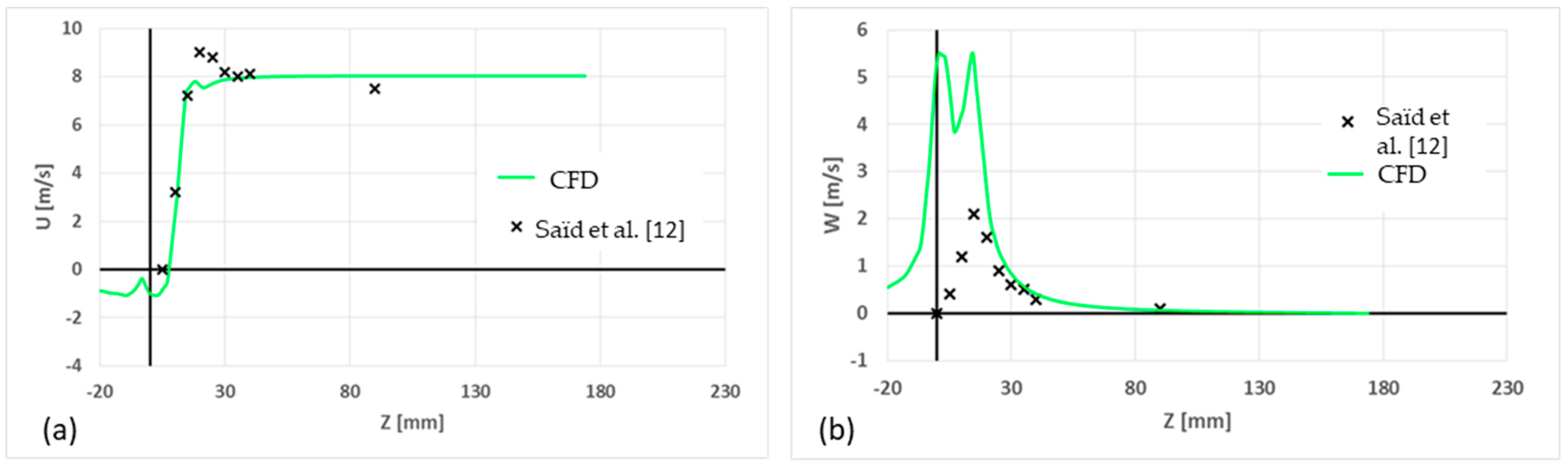
Figure 5.
Flow velocity components at section x = 16.7 [mm]—(a) U component and (b) W component [12].
Figure 5.
Flow velocity components at section x = 16.7 [mm]—(a) U component and (b) W component [12].

Figure 6.
Reynolds stresses at section x = 16.7 [mm]—(a) u’u’ component and (b) w’w’ component [12].
Figure 6.
Reynolds stresses at section x = 16.7 [mm]—(a) u’u’ component and (b) w’w’ component [12].

Figure 7.
Temperature contours in a cross-section as a function of vf.

Figure 8.
QoI detection zones—(a) control points set, (b) control surfaces set, (c) plume area.

Figure 9.
Temperatures recorded in the control points from DoE.

Figure 10.
Maximum temperatures from DoE.

Figure 11.
Plume cross-section area from DoE.

Figure 12.
Uniform distribution for the chimney exit flow velocity.
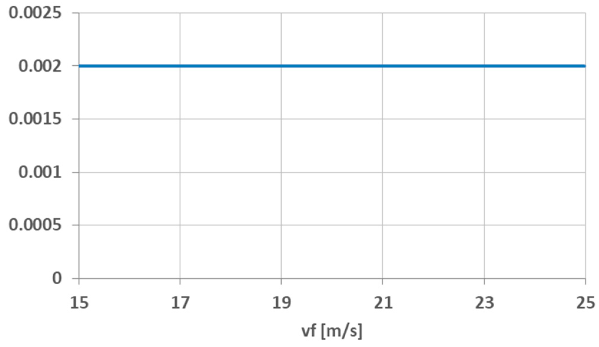
Figure 13.
Pdf of control point temperature measurements with uniform input distribution of vf.
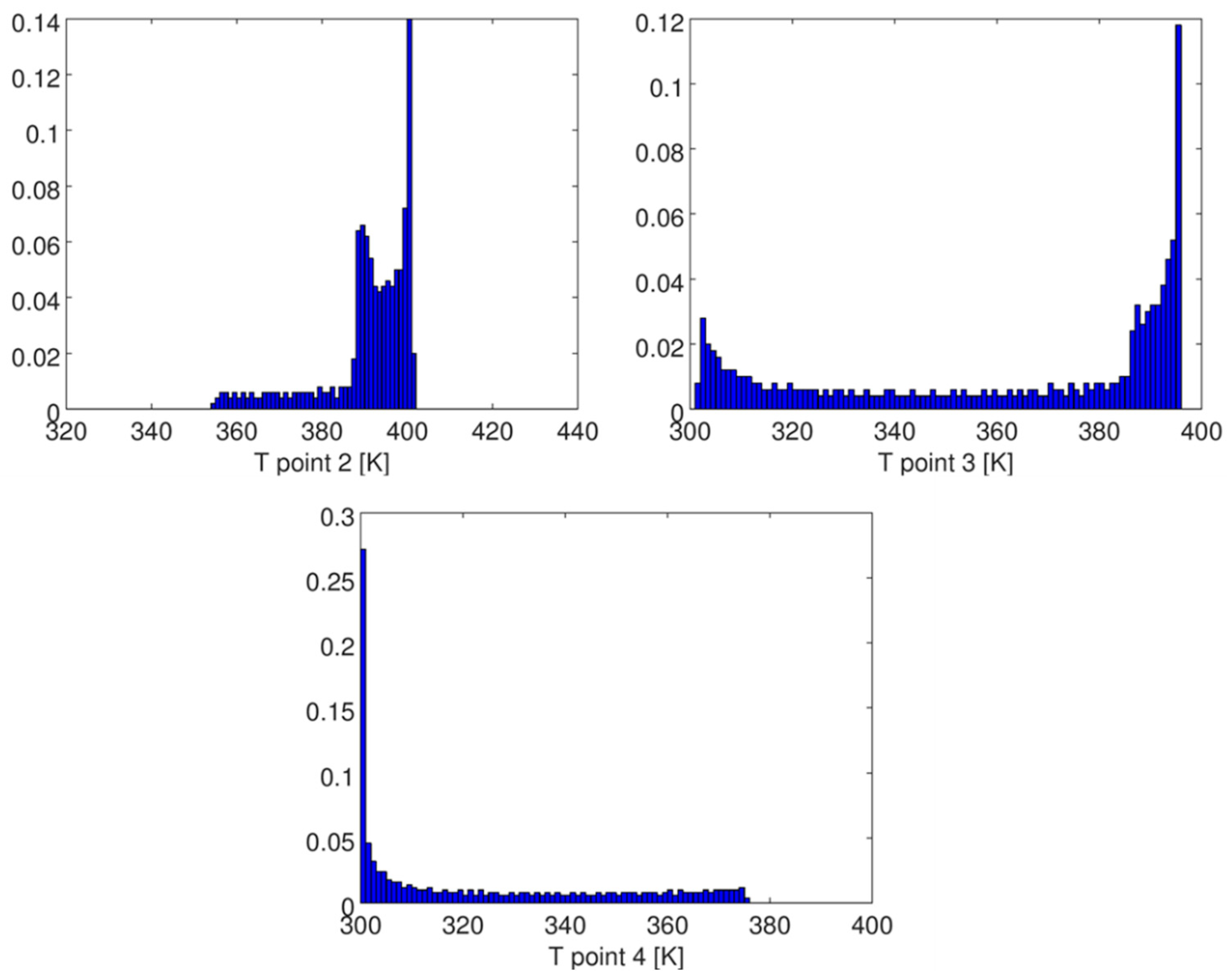
Figure 14.
Pdf of maximum temperature with uniform input distribution of vf.

Figure 15.
Pdf of cross-section area with uniform input distribution of vf.
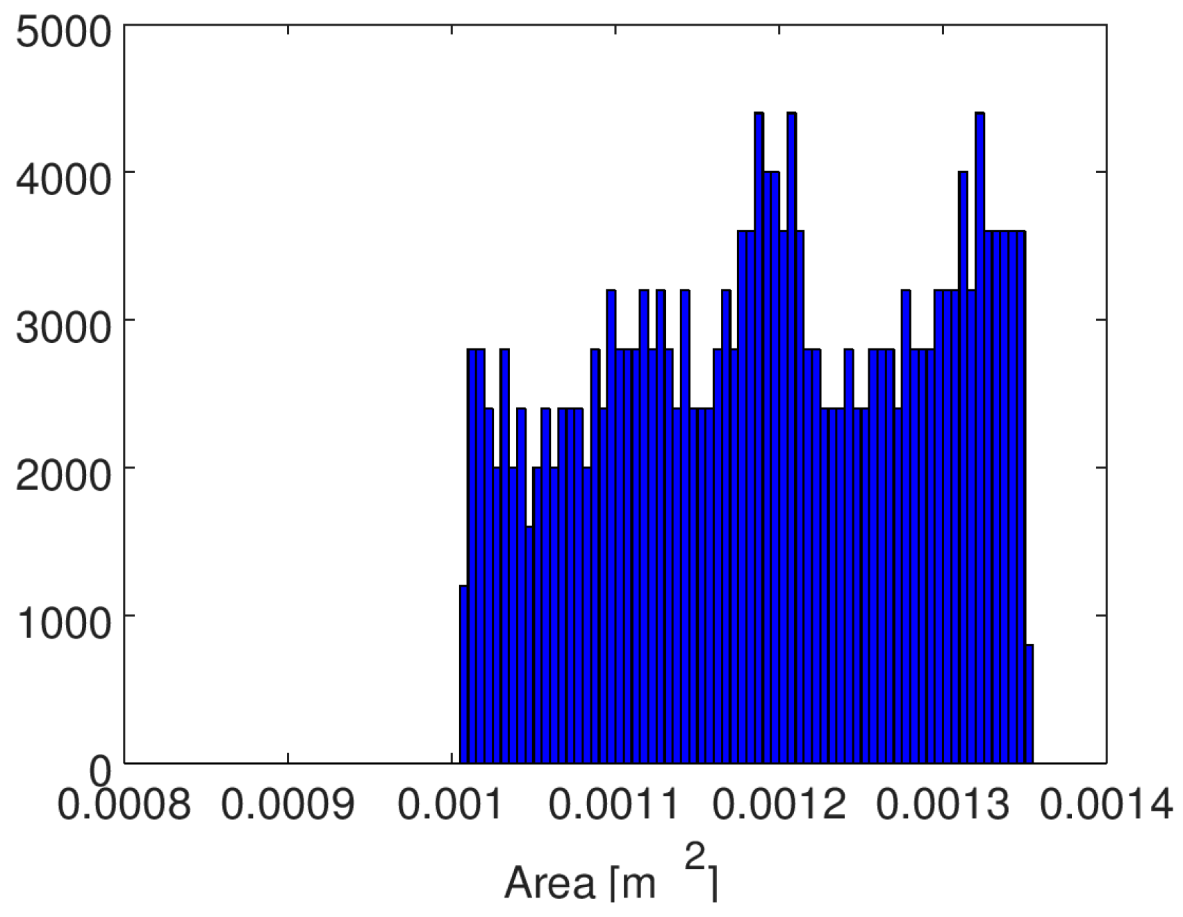
Figure 16.
Normal pdf input for the chimney exit flow velocity.
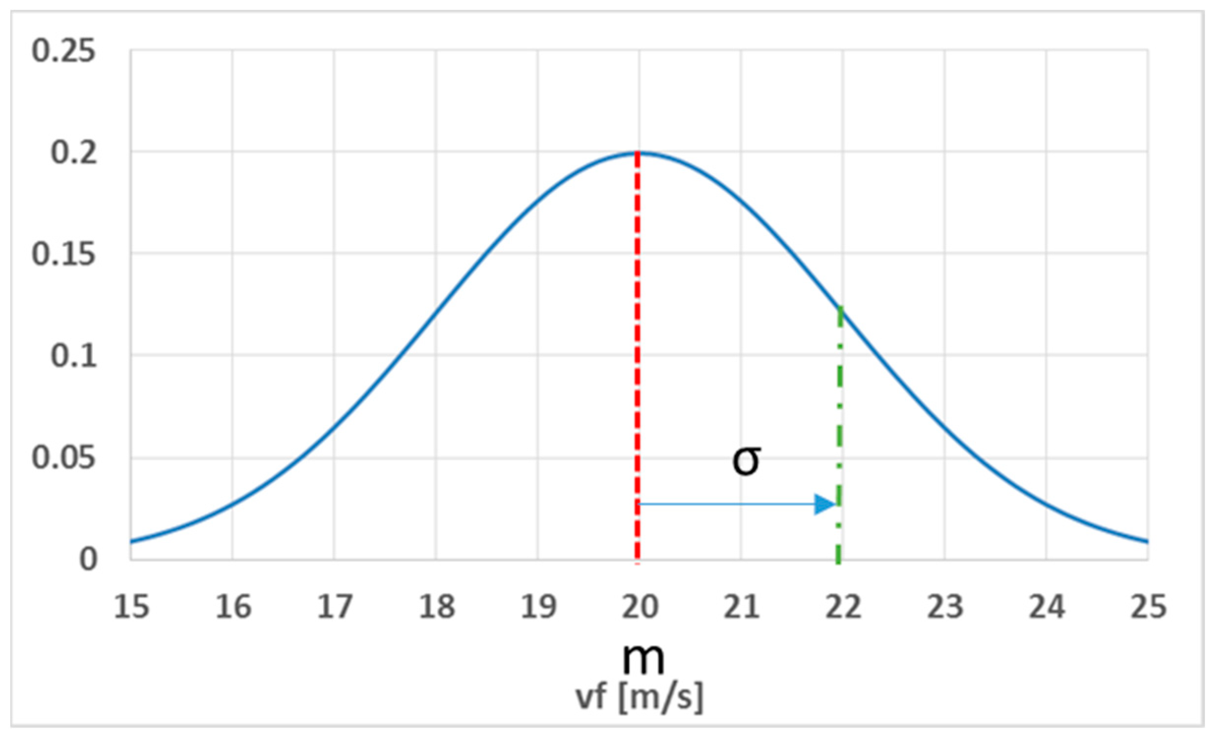
Figure 17.
Pdf on control point temperature with normal input distribution of vf.
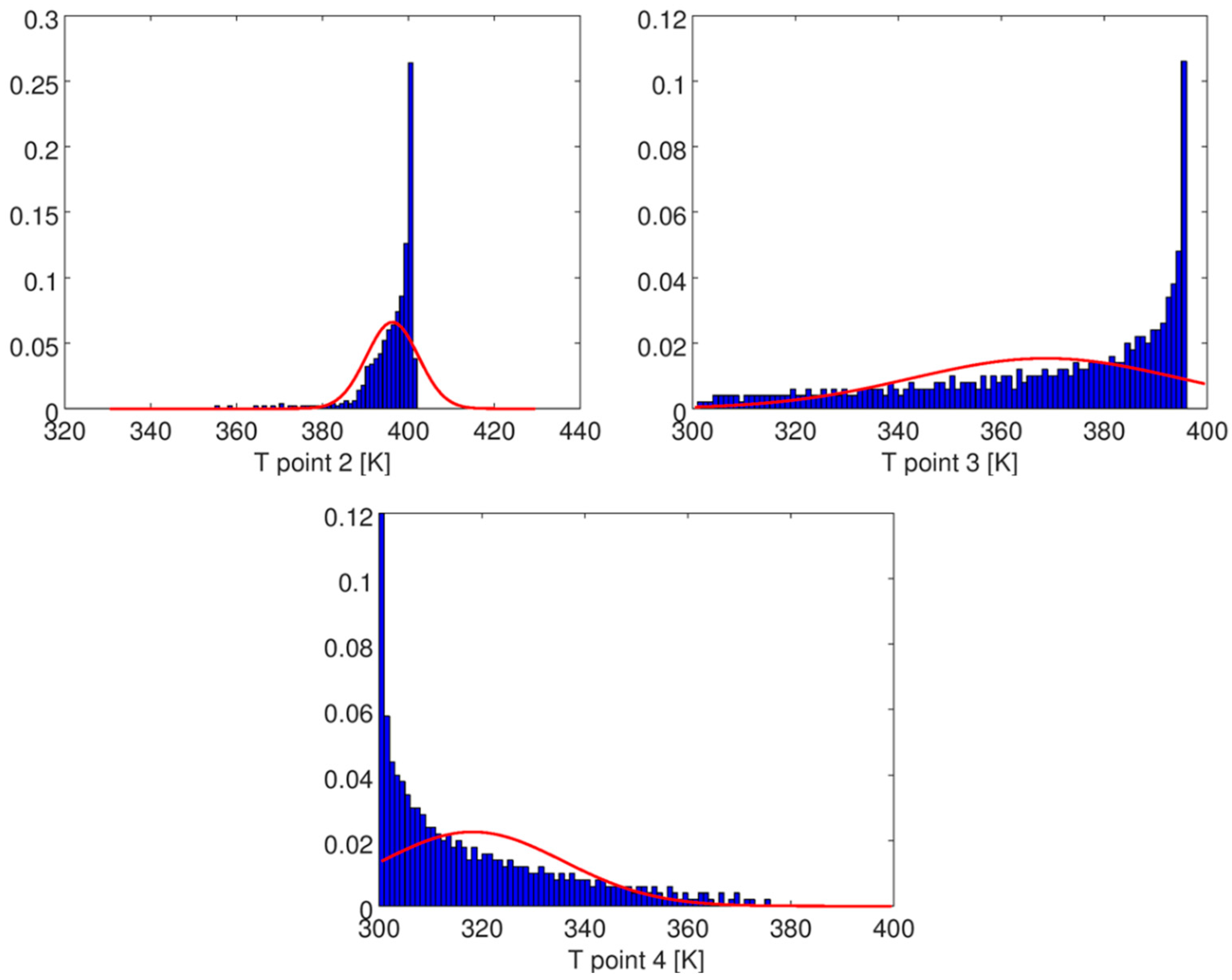
Figure 18.
Pdf of maximum temperature with normal input distribution of vf.
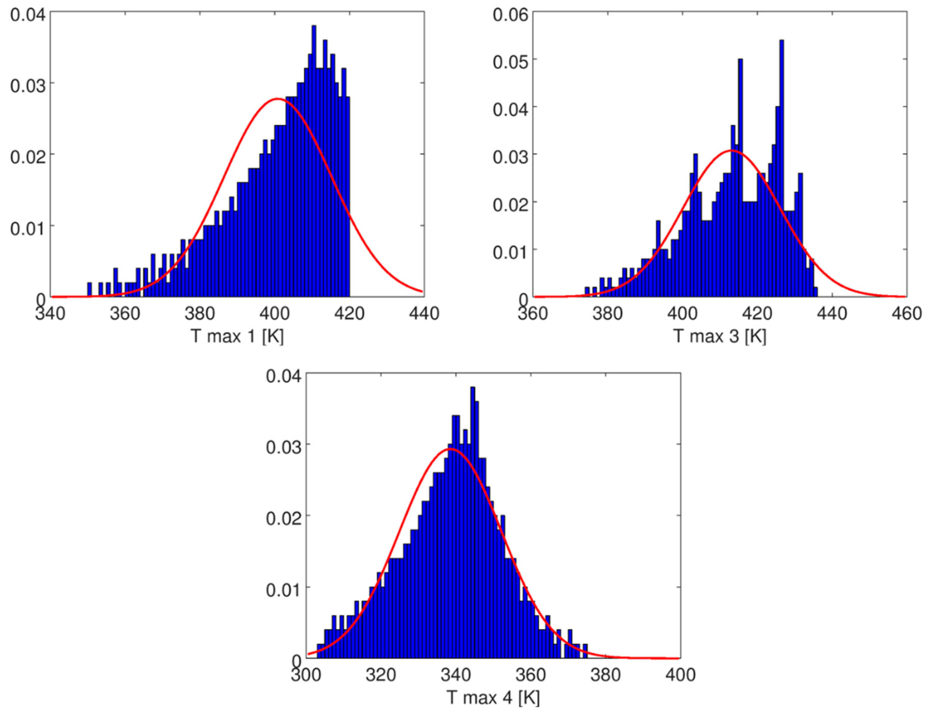
Figure 19.
Pdf of plume area with normal input distribution of vf.

Figure 20.
Comparison between surrogate-based and PCE results for certain QoI-exhaust gas outlet velocity.
Figure 20.
Comparison between surrogate-based and PCE results for certain QoI-exhaust gas outlet velocity.
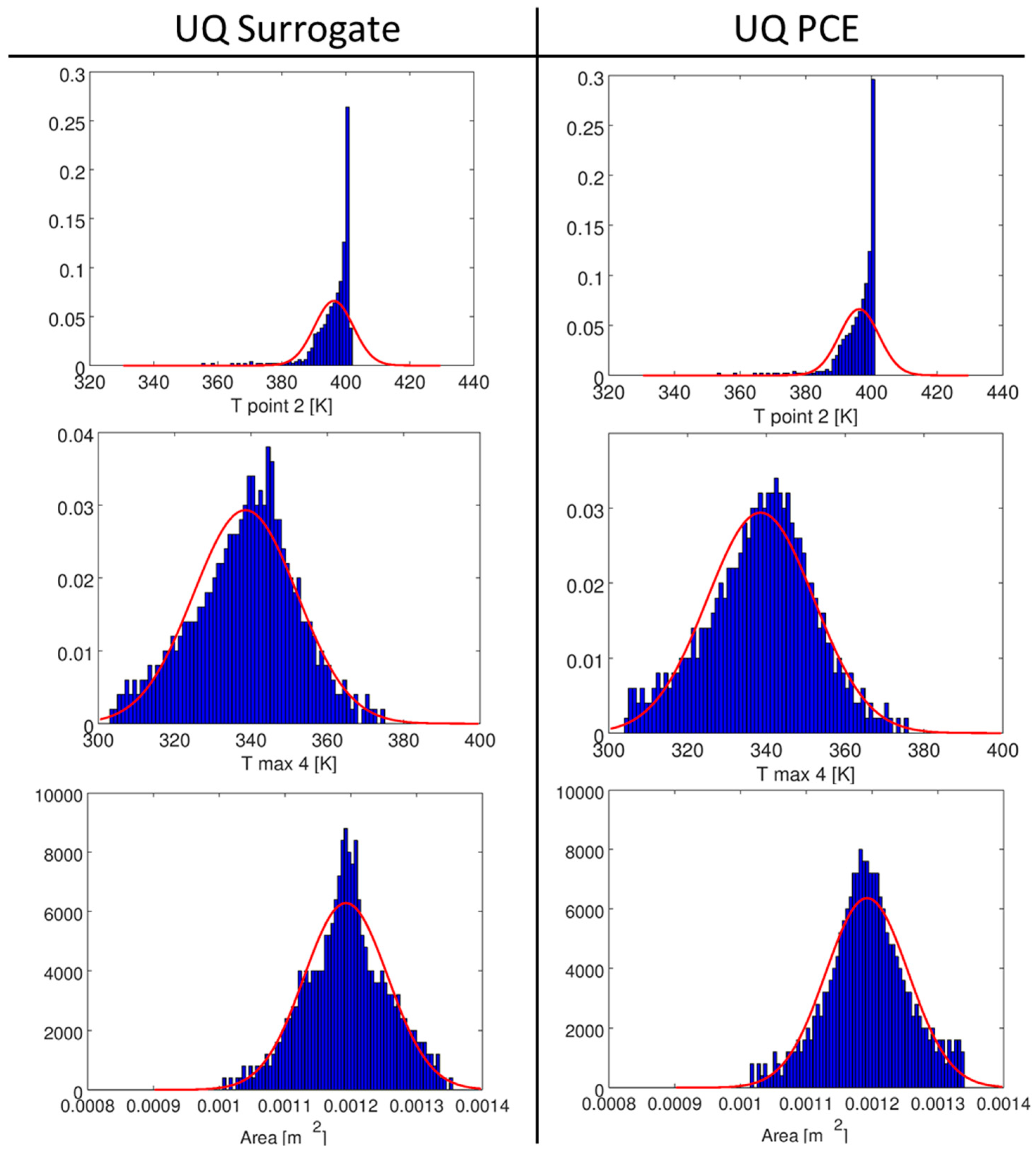
Figure 21.
Temperature contours in a cross-section as a function of wind direction α.
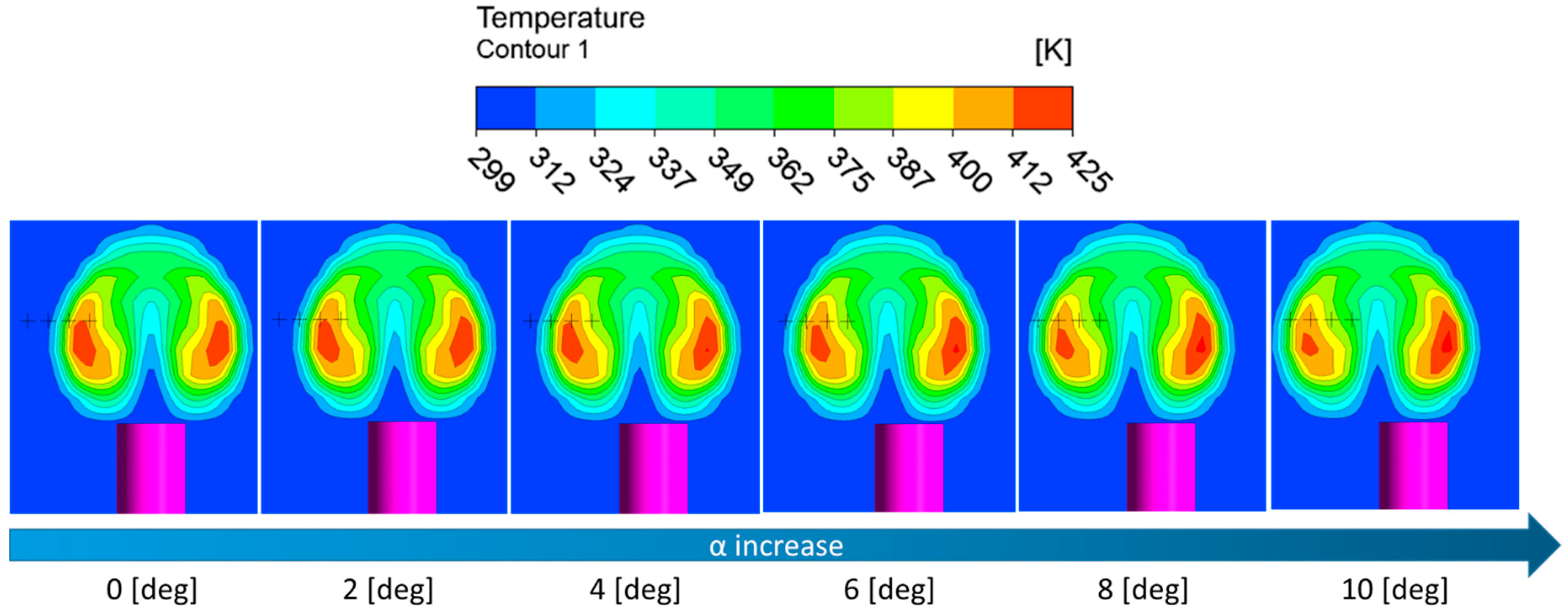
Figure 22.
Maximum temperatures from DoE—effect of incoming wind direction.
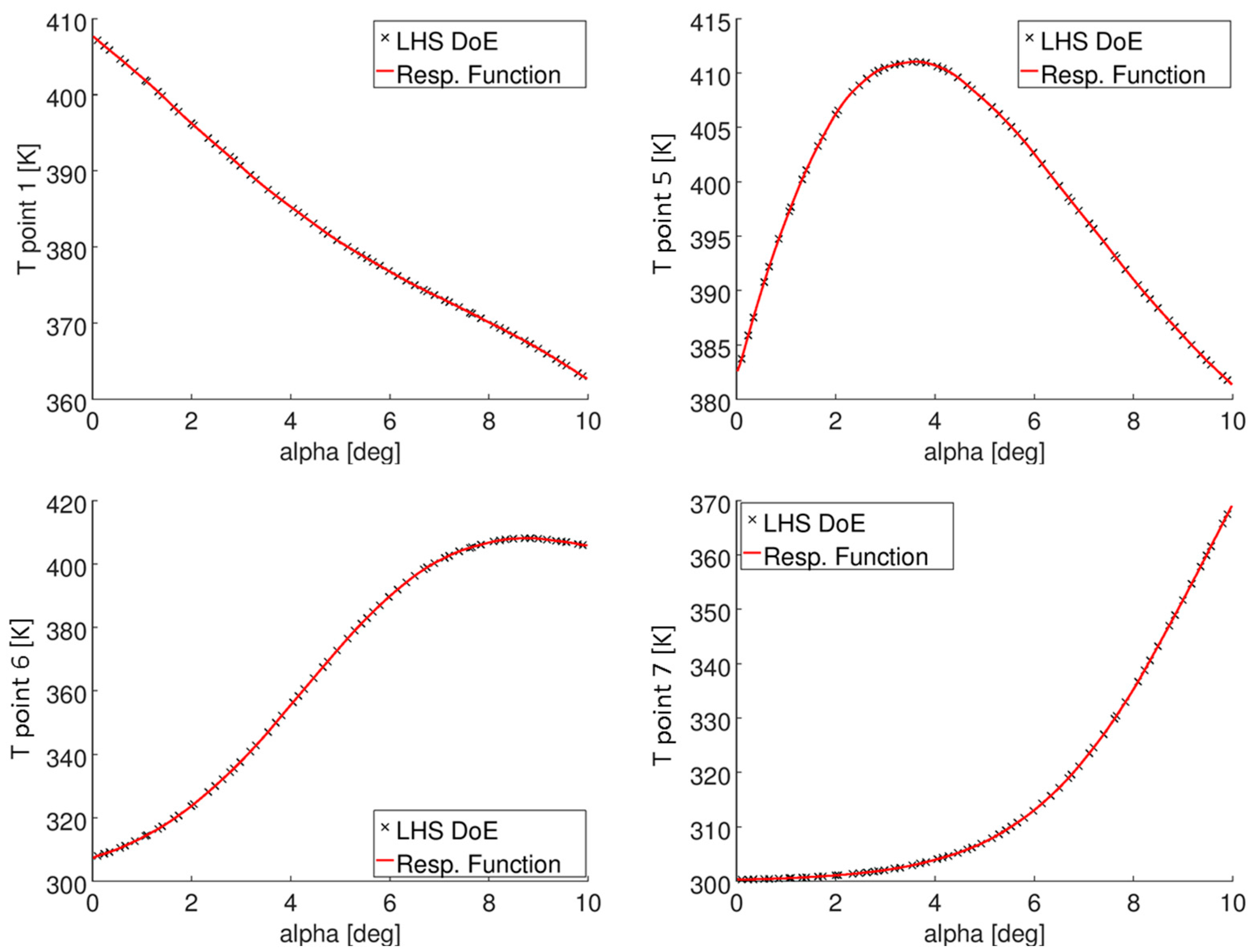
Figure 23.
Pdf of maximum temperature with normal input distribution of α.
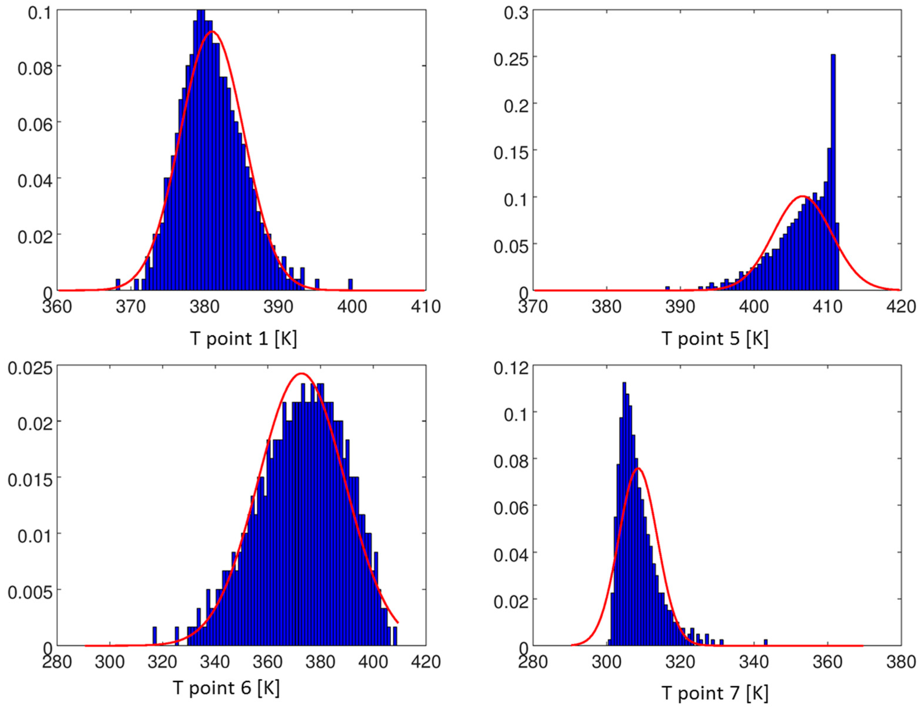
Figure 24.
Normal pdf input of flow angle.

Figure 25.
Comparison between surrogate-based and PCE results for certain QoI-wind direction.

Table 1.
Point probe coordinates.
| Detection Point | X (mm) | Y (mm) | Z (mm) |
|---|---|---|---|
| Point 1 | 30 | 9 | 15 |
| Point 2 | 30 | 9 | 20 |
| Point 3 | 30 | 9 | 25 |
| Point 4 | 30 | 9 | 30 |
| Point 5 | 30 | 12 | 15 |
| Point 6 | 30 | 15 | 15 |
| Point 7 | 30 | 18 | 15 |
Table 2.
Main statistical moments for the output probability density function distributions.
| Mean | σ | σ/m (%) | |
|---|---|---|---|
| Tmax,1 | 401 [K] | 14.3 [K] | 3.6 |
| Tmax,3 | 413 [K] | 12.9 [K] | 3.1 |
| Tmax,4 | 339 [K] | 13.6 [K] | 4.0 |
| Tpoint,2 | 396 [K] | 6.0 [K] | 1.5 |
| Tpoint,3 | 369 [K] | 26.0 [K] | 7.0 |
| Tpoint,4 | 318 [K] | 17.6 [K] | 5.5 |
| Area | 1.19 × 10⁻³ [m2] | 6.34 × 10⁻⁵ [m2] | 5.3 |
Table 3.
Main statistical moments for the output probability density functions.
| m (K) | σ (K) | σ/m (%) | |
|---|---|---|---|
| Tpoint,1 | 381 | 4.3 | 1.135 |
| Tpoint,5 | 406.5 | 3.9 | 0.975 |
| Tpoint,6 | 372.7 | 16.4 | 4.414 |
| Tpoint,7 | 308.5 | 5.2 | 1.704 |
Disclaimer/Publisher’s Note: The statements, opinions and data contained in all publications are solely those of the individual author(s) and contributor(s) and not of MDPI and/or the editor(s). MDPI and/or the editor(s) disclaim responsibility for any injury to people or property resulting from any ideas, methods, instructions or products referred to in the content. |
© 2023 by the authors. Licensee MDPI, Basel, Switzerland. This article is an open access article distributed under the terms and conditions of the Creative Commons Attribution (CC BY) license (https://creativecommons.org/licenses/by/4.0/).
Share and Cite
MDPI and ACS Style
Cravero, C.; De Domenico, D.; Marsano, D. Uncertainty Quantification Analysis of Exhaust Gas Plume in a Crosswind. Energies 2023, 16, 3549. https://doi.org/10.3390/en16083549
AMA Style
Cravero C, De Domenico D, Marsano D. Uncertainty Quantification Analysis of Exhaust Gas Plume in a Crosswind. Energies. 2023; 16(8):3549. https://doi.org/10.3390/en16083549
Chicago/Turabian StyleCravero, Carlo, Davide De Domenico, and Davide Marsano. 2023. "Uncertainty Quantification Analysis of Exhaust Gas Plume in a Crosswind" Energies 16, no. 8: 3549. https://doi.org/10.3390/en16083549
Note that from the first issue of 2016, this journal uses article numbers instead of page numbers. See further details here.