
Optimal Power Flow for Unbalanced Three-Phase Microgrids Using an Interior Point Optimizer
by
 ,
,
Piyapath Siratarnsophon
1,
Woosung Kim
2,
Nicholas Barry
3,
Debjyoti Chatterjee
2 and 
Surya Santoso
2,* 1
Department of Electrical Engineering, Faculty of Engineering at Sriracha, Kasetsart University, Chon Buri 20230, Thailand
2
Department of Electrical and Computer Engineering, The University of Texas at Austin, Austin, TX 78712, USA
3
Department of Electrical Engineering and Computer Science, United States Military Academy West Point, West Point, NY 10996, USA
*
Author to whom correspondence should be addressed.
Energies 2024, 17(1), 32; https://doi.org/10.3390/en17010032
Submission received: 27 November 2023
/
Revised: 13 December 2023
/
Accepted: 15 December 2023
/
Published: 20 December 2023
(This article belongs to the Special Issue Modeling, Optimization, and Control in Smart Grids)
Abstract
:Optimal power flow (OPF) analysis enables the in-depth study and examination of islanded microgrid design and operation. The development of the analysis framework, including modeling, formulating, and selecting effective OPF solvers, however, is a nontrivial task. As a result, this paper presents a tutorial on an OPF modeling framework, offering a mathematical model that can be readily implemented using established open-source software tools such as OpenDSS, Pyomo, and IPOPT. The framework is versatile, capable of representing single-phase and unbalanced three-phase islanded microgrids. Various inverter models, such as those of grid forming and following equipped with their operating characteristics, can be incorporated. The efficacy of the proposed framework is demonstrated in studying the OPF of single-phase and three-phase microgrids.
1. Introduction
The recent landscape of electrical power systems is marked by heightened complexity. OPF techniques are particularly well suited for addressing this augmented intricacy, accommodating the integration of distributed energy resources, battery energy storage systems (BESSs), and conventional generation sources. The application of OPF analyses has the potential to enhance microgrid design, streamline dispatch operations, and minimize generation costs, among other benefits. However, the task of developing and performing OPF analysis can be nontrivial. In particular, the inherent nonlinearity in the models of the microgrids poses challenges in the solution process. As a result, the OPF formulation needs to balance the complexity and accuracy. The designed mathematical formulation of the OPF needs to represent microgrids sufficiently accurately while simultaneously allowing for solution tractability.
Several research efforts focus on achieving a reliable solution for OPF by solving a simplified version of the original problem. The primary concept is to transform the OPF into a class of convex optimization problems, ensuring efficient computation and guaranteeing a global optimum. Three commonly employed convex relaxation techniques include semidefinite programming (SDP), second-order cone programming (SOCP), and quadratic convex (QC) relaxation. For instance, the application of SDP relaxation, as demonstrated in [1], involves removing the non-convex rank-one constraint to convert the original problem into a convex optimization. In [2], the quadratic equations were relaxed to inequality constraints, thereby convexifying the problem. The OPF problem can also be linearized, resulting in DC-OPF, which is typically employed by system operators to facilitate a reliable solution for performing economic dispatches. However, this relaxation may lead to significant errors [3].
While the relaxed OPF formulations and solutions provide effective approaches for achieving global optimal solutions, most of them are developed for single-phase or positive-sequence networks [4]. Additionally, the relaxation may not always be exact, particularly in cases where the underlying network is not radial. An example of this scenario arises when the rank-one constraint in the SDP relaxation is not met [5]. These relaxed OPF methods may not offer accurate modeling of general, unbalanced, three-phase islanded microgrids [6]. Furthermore, although the solution process is optimal and typically efficient, the solutions obtained may not fully reflect the characteristics of the original systems.
Another research effort, such as in [7,8,9], acknowledges the inherent nonlinearity and non-convexity of the OPF. The overall OPF is identified as a nonlinear programming problem (NLP) that can be solved by employing some nonlinear solution methods. With the advancement of numerical methods and robust nonlinear solvers, OPF problems can incorporate more intricate models to improve modeling accuracy.
One such improvement involves the incorporation of the droop control characteristics of inverters to improve the model accuracy of the islanded microgrid operation [10,11]. Additionally, the active and apparent power limits of inverters can also be modeled to simulate the practical operation of droop control. This additional modeling, however, presents a challenge, as it introduces additional nonlinearity to the formulation, thereby increasing the difficulty of solving for the OPF. Various modeling approaches have been proposed. The first approach employs an algorithm similar to PV (voltage-controlled generator) and PQ (load) bus type switching. Nonetheless, this method may encounter numerical issues, leading to solution divergence [12,13]. In the second approach, integer variables may be introduced as indicators for the operational mode of inverters [14,15]. This approach, however, transforms the original OPF to a mixed-integer nonlinear programming problem, which is generally more challenging to solve.
Alternatively, the authors of [16,17,18] modeled the inverter limits with nonlinear complementary problem (NCP) constraints. The inverter limits are encompassed in Fischer–Burmeister (FB) functions. However, as the FB function is non-smooth, the direct application of a Newton-like method to solve for the OPF is hindered. In [17], a semi-smooth modified Newton-like method was adopted to directly solve for the OPF [18].
As discussed above, creating an accurate model of the OPF is a complex task that involves numerous microgrid components. Moreover, implementing OPF for an islanded microgrid can be a cumbersome process, requiring the development of physical system models, optimization formulations, and an optimization solver. Motivated to simplify the development process, this paper aims to provide a comprehensive tutorial of an OPF modeling framework. An OPF formulation that is general and capable of accommodating both single-phase and three-phase islanded microgrids, along with various inverter types and limit considerations, is presented. This framework is designed to facilitate straightforward development using open-source software and packages.
Section 2 provides an overview of the microgrids’ OPF analysis. The OPF modeling and analysis framework is presented in Section 3. Detailed models of the OPF for microgrids and their components are presented in Section 4. Section 5 and Section 6 offer demonstrations of the OPF modeling and analysis. The conclusion is provided in Section 7.
2. Background
This section provides a broad understanding of microgrids, encompassing their key components and typical steady state analyses.
2.1. Microgrid Components
Microgrids comprise three fundamental components: power delivery elements (PDEs), demand, and generation. PDEs such as distribution lines and transformers constitute the essential infrastructure for distributing electrical energy from generators to loads. A microgrid may incorporate various types of generation resources, such as BESSs and photovoltaic systems (PVs). Beyond their role as generators, these inverter-based resources (IBRs) can also be employed to enhance microgrid operations, leveraging their flexible active and reactive power control capabilities. As per [19], IBRs can be categorized based on their inverter controls into four types:
- Current source inverters maintain a constant power output regardless of the voltage level at the point of common coupling (PCC). This type of inverter functions similar to traditional power generation units.
- Voltage source inverters regulate both the system frequency and PCC voltage, acting as stabilizing agents in microgrid operation.
- Current source grid-supporting inverters share similarities with current source inverters in regulating their constant power output. However, their active and reactive power can be adjusted based on the system frequency and PCC voltages to support the grid.
- Voltage source grid-supporting inverters regulate the PCC voltage and frequency, resembling voltage source inverters. However, their setpoints are adjusted depending on their supplied active and reactive power.
In this paper, the primary modeling and analysis focus on islanded microgrids. This entails a specific focus on the modeling of voltage source grid-supporting and current source grid-supporting inverters, which will be denoted as the grid-forming inverter (GFM) and grid-following inverter (GFL) for clarity in subsequent discussions, respectively.
2.2. Microgrid Steady State Modeling and Analysis: Power Flow and Optimal Power Flow
Power flow (PF) and OPF analyses can be applied to examine the steady state operating conditions of microgrids. In PF analysis, the dispatches of IBRs are fixed. The goal of the analysis is to determine the resulting operating conditions. Subsequently, additional analyses may be performed to confirm compliance with established standards and operating requirements. Evaluation may encompass aspects such as voltages, equipment ratings, and the system frequency, which are crucial for the operation of microgrids.
In contrast to the PF analyses, OPF studies typically yield non-deterministic solutions when their objectives are not incorporated. Their goal is to identify the optimal values of the control variables under given objectives. This may involve optimizing active and reactive power dispatches of IBRs to minimize operating costs or system losses. Notably, OPF analyses are more flexible and comprehensive. They can be streamlined into PF studies by fixing their decision variables (e.g., dispatches of IBRs).
3. OPF Modeling Framework
In this section, an example of OPF modeling and its implementation framework are presented. The implementation utilizes the following established open-source software:
- OpenDSS [20] is open-source software for simulating and analyzing electrical distribution systems. It is used to model microgrids and their components, such as transformers, lines, capacitors, distributed generators, and loads. Its extensive libraries provide modeling flexibility and facilitate fast development.
- Pyomo [21,22] is an open-source Python package that provides a wide range of optimization tools for formulating and analyzing models. Its application of symbolic definitions and multi-dimensional parameters and variables offers flexibility in modeling. Additionally, Pyomo provides an interface prompt of various solvers like Gurobi, IPOPT, and BONMIN to conveniently solve the formulated problem. In this modeling framework, Pyomo is employed to implement the OPF formulation. This formulation encompasses an objective function and constraints for modeling the microgrid network, its electrical components, and the operating requirements.
- Interior Point Optimizer (IPOPT) [23] is an open-source software package designed for nonlinear optimization. This solver is adopted in this modeling and analysis framework for its robustness. The objectives and constraints can be linear or nonlinear and convex or non-convex.
The overall OPF modeling framework is as illustrated in Figure 1. The initial modeling step involves using OpenDSS to model the microgrid circuits. During this phase, various electrical components such as lines, transformers, loads, PVs, and BESSs are integrated into the model. Once the microgrid model is established, a basic power flow analysis can be performed to assess a snapshot overview of the microgrid’s operational condition. Subsequently, in the second modeling step, relevant circuit parameters, such as the system admittance matrix and specific details of each electrical component, can be extracted from the OpenDSS model to formulate an OPF problem. In this step, controls or specifications for the electrical components and the system operation requirement constraints that are not reflected in the OpenDSS model can also be incorporated. Finally, Pyomo interfaces with the IPOPT solver to effectively solve the formulated OPF.
4. OPF Modeling and Formulation
This section presents the mathematical model for microgrid systems and IBRs, as well as the overall formulation of the OPF.
4.1. Nomenclature
4.2. Microgrid Network
A microgrid network can be modeled using the active and reactive power balance at each node:
The conductance and susceptance of each PDE can be queried from OpenDSS. In this modeling framework, it is assumed that the change in system frequency has no impact on admittance. Therefore, the conductance and susceptance are considered constant for modeling and analysis purposes.
4.3. Grid-Forming Inverter-Based Resource
Modeling the GFM involves capturing the steady state relationship of the droop control characteristic and the system conditions at the PCC. The GFM models are presented for both the single-phase and three-phase configurations.
4.3.1. Single-Phase Grid-Forming Inverter-Based Resource
The mathematical representation of a single-phase GFM s connected to an electrical node i with grid-supporting functionality is expressed as follows:
Equations (3) and (4) describe the droop control characteristic of the GFM. The limits in kW or kVA for the IBR are modeled in Equations (5) and (6), respectively. For the designated GFM , an additional equation (Equation (7)) is provided to model the angle reference of the islanded microgrid, similar to the slack bus in traditional power flow analysis.
4.3.2. Three-Phase Grid-Forming Inverter-Based Resource
Modeling of the three-phase GFM presents additional complexity due to the intricacies of its voltage control system. Various control schemes exist for GFMs, ranging from those incorporating negative-sequence voltage control to those with virtual impedance. In this work, the three-phase GFM is assumed to solely employ the positive-sequence voltage control scheme. With this scheme, GFMs consistently maintain balanced PCC voltages regardless of the loading conditions. Specifically, during unbalanced loading conditions, the PCC voltages remain balanced, despite the unbalanced current and power supplied at the PCC. The model of a three-phase GFM s connected to phases A, B, and C at nodes a, b, and c, respectively, can be expressed as follows:
Equations (8) and (9) establish the relationship between the total active and reactive power, respectively, with respect to the droop control. Equations (10) and (11) describe the controlled balanced voltage output at the PCC of the GFM. Lastly, Equations (12) and (13) model the kW and kVA limits of the GFM, respectively. Additionally, at the designated three-phase GFM denoted by , Equation (14) is included to provide the angle reference for the islanded microgrid, akin to the role of the slack bus in traditional power flow analysis.
4.4. Grid-Following Inverter-Based Resource
Similar to GFM modeling, GFL modeling involves capturing the steady state relationship between the inverter control characteristics and the system conditions at the PCC. However, there are several key distinctions. In this work, the GFL may operate at its operational limits, effectively emulating constant power behavior. In contrast, the GFM is assumed to always operate within its ratings to ensure the security of the islanded microgrid. Additionally, the control strategy for the three-phase GFL differs from that of the three-phase GFM, owing to the contrasting control paradigms between the current source and voltage source inverters.
4.4.1. Single-Phase Grid-Following Inverter-Based Resource
The model of a single-phase GFL k connected at a node i, neglecting considerations for the inverter capacity or power limits, can be expressed as follows:
The model of the single-phase GFL without operating limits closely resembles that of the GFM. However, when factoring in the operational limits of the GFL, the modeling becomes more complicated. Consider the characteristic of the active power injection of a GFL with a kW limit:
It can be observed that a conditional model is necessary, as the GFL must operate only in one operating mode, depending on whether the calculated droop power falls within the lower and upper active power ratings.
One approach to achieve this desired conditional model is employing algorithms similar to PV (voltage-controlled generator) and PQ (load) bus type switching. This involves assuming an operational mode of the GFL, executing the OPF analysis, and validating the assumed operational mode. If the validation fails, then the models are adjusted, and the OPF is reevaluated.
However, for simplicity in modeling and implementation, the proposed modeling framework adopts an alternative approach that employs the Fischer–Burmeister (FB) function [24] to represent the conditional model of the GFL’s operating limits. The FB function : is defined as follows: . Here, the solutions to fall into two sets: (1) and or (2) and . This key characteristic facilitates the conditional modeling of the GFL’s limits. In particular, the lower kW limit can be modeled by setting and . As a result, the two solution sets of are as follows:
- and : the power injection of the GFL is limited to the minimum kW rating when the power calculated from the droop control is less than the minimum kW limit ().
- and : this solution set describes the scenario where the GFL power is set to the droop power calculation when the calculated droop power is greater than the minimum kW limit.
Overall, both the upper and lower kW limits can be modeled by augmenting two smooth FB functions such that .
However, since the FB function is not smooth and is not suitable for the IPOPT solver [23], this presented formulation opts for the smooth FB function instead, where :
Here, is a small designed parameter. According to [24], also represents the modeling error between the smooth function and the original FB function. In particular, . Similar to the kW limit, the kVA limit of the GFL can be modeled using the smooth FB function. The single-phase GFL k model connected to electrical node i with kW and kVA limits can be expressed as follows:
where . Equations (18) and (19) calculate the target active and reactive power injection according to the droop control, respectively. Equations (20) and (21) model the active and reactive power injection considering the GFL limits, respectively.
4.4.2. Three-Phase Grid-Following Inverter-Based Resource
Unlike the GFM, the GFL employs current control rather than voltage control. There are multiple control schemes for GFLs, such as positive negative sequence compensation (PNSC) and balanced positive sequence control (BPSC) [25]. In this paper, the BPSC scheme is adopted. Under this control scheme, balanced current injection is calculated from the positive sequence voltage and three-phase power. Despite the balanced current, the power injection at the PCC may be unbalanced if the PCC voltage is unbalanced. The mathematical model of a three-phase GFL k connected to nodes a, b, c at phases A, B, and C, respectively, can be expressed as follows:
where , , and . Equations (22)–(24) calculate the positive sequence voltage at the PCC. Equations (25) and (26) represent the total active and reactive power injection targets based on the droop control, respectively. Equations (27) and (28) model the actual total power output after accounting for the kW and kVA limits, respectively. Equations (29)–(34) model the power per phase injection.
4.5. BESS State of Charge
In addition to the inverter models, the state of charge (SoC) of a BESS e connected to electrical nodes can be calculated as follows:
where is the power injection of the BESS e at its node connection i, which is for the GFM BESS () or for the GFL BESS ().
4.6. Operational Constraints
Aside from the microgrid network model and its components, acceptable system operation operational constraints should also be modeled. These constraints may encompass the lower and upper limits of the voltage, system frequency, and SoC, which can be expressed as follows:
The line loading limit of a PDE l connected to node can be expressed as follows:
where and represent the real and imaginary components of the current flowing at node i of PDE l, respectively. The conductance and admittance of a PDE l can be obtained from OpenDSS.
4.7. Objective
The objective function of this OPF formulation is generally set to minimize the deviation of the IBR’s operating conditions from their target setpoints. The selection of costs and target setpoints should reflect the focus and application of the OPF objectives. For maintaining the microgrid’s secure operation, the target BESS SoC levels should align with a capacity capable of meeting the expected demand or absorbing generation from non-controlled sources. To enhance efficiency and minimize losses, the IBRs’ target power setpoints can be set to zero. Alternatively, they may be set according to prearranged agreements. For example, the target active power can be selected following predetermined economic dispatches. For IBRs providing ancillary services like voltage support or power factor correction, nonzero reactive power setpoints may be selected. To prioritize different deviations, varying costs can be assigned, with a higher cost indicating a preference for less deviation. Overall, the expression for the objective function is as follows:
where the total active or reactive power of the GFM or GFL is calculated by summing the power injection to all of their connected nodes.
4.8. OPF Formulation
The overall formulation is presented in Equation (43). This formulation comprises both the objective function and the set of constraints. The constraints encompass models of the microgrid network, single-phase and three-phase GFMs and GFLs, as well as the system’s operational requirements:
The proposed formulation is applicable for both OPF and PF analyses. In an OPF study, the IBR dispatches, along with other variables, are collectively optimized under the specified objective function and subject to the relevant constraints.
In contrast, in a PF study, the dispatches of all IBRs are predetermined, resulting in a deterministic solution. Therefore, the objective in PF studies is irrelevant and is typically set to minimize to zero. The primary aim of a PF study is to investigate the operating conditions resulting from the IBR dispatches.
Furthermore, while the above formulation is tailored for snapshot analysis, it can be seamlessly extended for quasi-static time series (QSTS) studies by solving a series of snapshot OPFs. At the beginning of each planning interval, the microgrid conditions such as the load, PV, or BESS SoC are adjusted before the OPF analysis is carried out.
5. Demonstration I: A Single-Phase Three-Bus Islanded Microgrid
In this section, the application of the proposed modeling framework to conduct PF and OPF studies in an islanded microgrid is presented. The capability and verification of the proposed framework are demonstrated through study scenarios involving a simple single-phase three-bus islanded microgrid.
5.1. Microgrid Details
The demonstration islanded microgrid circuit was as illustrated below in Figure 2. The system was a simple single-phase three-bus 240 V system where the nominal frequency was 60 Hz. Two circuit variations were considered. In the first circuit variation (Microgrid I), there was a GFM BESS at Bus 1 and a PV GFL (PV1) at Bus 3. There were three identical loads at each bus. In the second variation (Microgrid II), there was an additional PV (PV2) at Bus 2 also operating as a GFL. and for all IBRs were set to 240 V and 60 Hz, respectively. The admittance and were S and S, respectively. The current limit of all PDEs was 100 A. The lower and upper limit of the SoC were 0% and 100%, respectively. The details of the IBRs and loads are summarized in Table 4.
5.2. Verification of the OPF Modeling Framework
For verification, the PF and OPF results of the islanded microgrid obtained through the proposed approach will be compared with the methodology outlined in [26]. In this referenced approach, the power flow solution of an islanded microgrid is computed through iterative updates between the power flow solution obtained using OpenDSS and IBR models implemented in Python. The OpenDSS solution provides essential microgrid operating parameters, including the voltage magnitudes and angles, contingent on the setpoints of the IBRs. Concurrently, the IBRs recompute their outputs, considering their controls and inverter limits, in response to the microgrid operating conditions. Power flow of the islanded microgrid is computed when the iterative process converges. As PF analysis was the focus of the reference approach, optimization and implementation with Pyomo and IPOPT was not necessary. In the subsequent discussions, the accuracy of the proposed modeling approach will be evaluated by analyzing the percentage difference error in power flow results compared with the referenced approach.
5.3. Studied Scenarios
In Demonstration I, three scenarios are provided to illustrate various facets of the proposed modeling and analysis approach. Scenarios I and II focus on modeling of the GFL and GFM in snapshot power flow analyses. Scenario III considers all inverter limits and provides a demonstration for executing QSTS analyses for both PF and OPF analyses.
5.3.1. Scenario I: PF Analysis of Various GFL Models
In Scenario I, three analyses are performed on Microgrid I, exploring various GFL setpoints and limits. The details of each case, including the corresponding OPF constraint models, are presented in Table 5. Pyomo was employed to model the OPF constraints in each case, and the PF results were obtained through solving the OPF without an objective using IPOPT. Case 1.1 involves a power flow study without considering the GFL limits, while Case 1.2 incorporates the GFL kW limit. In Case 1.3, both the kW and kVA limits of the GFL are modeled. In all cases, the GFM BESS operating limits are not considered. Its active and reactive power setpoints were configured to zero. Furthermore, the BESS initial SoC level was 100%. The voltage and frequency operating constraints were not considered in this simulation to focus on GFM and GFL modeling.
Table 6 presents the power flow solutions for the study cases, including the active and reactive power generation of the BESS and PV, system voltage magnitudes, frequency, and BESS SoC after 15 min. The presented active and reactive power followed the generator convention, where positive kW generation indicates discharging of the BESS. It can be observed that the proposed model effectively ensured the active and apparent power of the GFL when the limits of the model were applied. In Case 1.2, the active power of the GFL was limited to 10 kW, while in Case 1.3, both the active and apparent power were restricted to 10 kW and 14 kVA, respectively. The summary of the verification error differences between the proposed modeling approach and the reference, as presented in Table 7, indicates a high degree of agreement between the two methods, with errors below 0.1%.
5.3.2. Scenario II: PF Analysis of Various GFM Models
Scenario II focuses on demonstrating the modeling of a GFM. Various setpoints of the GFM, as detailed in Table 8, were simulated in Microgrid I. The and setpoints of the GFL were configured to 0 kW and 0 kvar in all cases. In Scenario II, the power flow of the islanded microgrid was determined both with and without the GFM limits.
With the GFM limits, feasible power flow solutions accurately reflect the operating condition of the islanded microgrid. On the other hand, an infeasible solution may imply that the microgrid may not be operable. Additionally, a power flow solution without the GFM limits was also performed for validation with the referenced approach. In this case, the results of the power flow could be used to investigate the infeasibilities of operating the GFM.
The power flow of the islanded microgrid with all GFM limits could be determined with the proposed analysis framework by solving an OPF without objectives. The OPF formulation is as follows:
Similar to the implementation in Scenario I, the PF results of each case could be obtained by formulating the OPF models using Pyomo and then solving them with IPOPT. To simulate the power flow without the GFM limits, the constraints in Equations (5), (6), and (38) were neglected while solving for the OPF. Similar to Scenario I, the voltage and frequency operating constraints were not considered.
Table 9 and Table 10 display the power flow results and the corresponding percentage difference errors relative to the referenced approach without considering the GFM limits, respectively. It can be observed that the results for both approaches aligned with errors differing by less than 0.5%. The power flow results indicate that the islanded microgrid could operate without any violations in Case 2.1 and Case 2.2. However, in Case 2.3, the GFM’s SoC fell below 0%. Additionally, in Cases 2.4 and 2.5, the GFM’s active power and apparent power exceeded its kW and kVA ratings, respectively. Simulations conducted using the proposed framework with the GFM kW and kVA limits yielded feasible power flow solutions, consistent with the results obtained without the GFM limits for Cases 2.1 and 2.2. On the other hand, the OPF produced infeasible power flow results for Cases 2.3, 2.4, and 2.5, confirming that the islanded microgrid was not operable in those cases.
5.3.3. Scenario III: QSTS PF and OPF Analyses
In Scenario III, QSTS analyses with PF and OPF are demonstrated on an islanded microgrid (Microgrid II). The load demand and PV generation levels were varied throughout the day. The analysis was performed in 15 min intervals starting at 6:30 a.m. Both the PF and OPF analyses started from the same initial circuit conditions and continued until the microgrid became inoperable, as indicated by voltage or frequency violations or the insufficient capacity of the GFM BESS. The maximum voltage and frequency deviations were 5%, and 7% from the nominal values, respectively.
In the PF analysis, the droop active and reactive power setpoints for the BESS were both configured to zero. Meanwhile, for the PVs, the droop active power setpoint was adjusted to match the maximum power generation based on irradiance, while the droop reactive power setpoint was set to 0 kvar.
On the other hand, in the OPF analysis, the droop setpoints for the PVs remained the same as those in the PF analysis. However, the active and reactive power setpoints of the BESS were optimized with the objective of keeping the SoC at 95%. Additionally, the objective also minimized the usage of reactive power for the BESS. The cost coefficients and were set to 100 (USD) and 0.01 (USD/), respectively. The formulation is as follows:
Figure 3 and Figure 4 present the QSTS simulation results of the PF analysis, including profiles of the power, system voltages, frequency, and BESS SoC level. Figure 3b shows the progression of the BESS SoC level and system frequency over time. It can be observed that the microgrid could maintain islanded operation until 8:15 p.m. before the microgrid frequency dropped below the operating limit. In Figure 3a, the total active power profile, categorized by resource type throughout the analysis period, is illustrated. The total demand (demand) consistently remained around 10 kW throughout the day. The BESS generation profile (es_gen) shows that the BESS achieved a maximum charging rate of less than 5 kW during the afternoon. Additionally, it can also be observed that the active power output of the PVs (pv_gen) was curtailed from their available generation (pv_gen_available). In Figure 4a, the system voltages are shown to be within the operating requirement during the entire islanded operation. Additionally, in Figure 4b, the effectiveness of droop control in coordinating the PVs and BESS to supply reactive power to the loads is illustrated.
The QSTS results for the OPF analysis are shown in Figure 5 and Figure 6. Similar to the PF analysis, the profiles of the power, system voltages, frequency, and BESS SoC level are provided. With the optimized BESS droop settings for active and reactive power, the OPF analysis indicates that the microgrid could remain in islanded operation for an additional 150 min before the ES SoC depleted.
In Figure 5a, it can be observed that the BESS charged at its full kW rating and reached its target SoC after 1:30 p.m. Subsequently, the and dispatches of the BESS were adjusted to maintain the BESS SoC at the target level until 7:30 p.m., when its generation was required due to insufficient PV power to supply active power to the load. Figure 6b illustrates the effective coordination of the IBRs in supplying reactive power to meet the demand. Additionally, Figure 6a shows that the overall system voltage was slightly lower when the BESS charged at its full kW rating. However, the voltages throughout the entire islanded operation remained within the operating requirements.
5.4. Discussion
In this section, demonstrations of snapshot and QSTS analyses for the PF and OPF of single-phase islanded microgrids utilizing the proposed modeling framework are presented. In Scenarios I and II, the proposed OPF modeling framework was applied to analyze the snapshot PF of Microgrid I, taking into account variations in the GFM and GFL inverter limits. The comparison of the resulting microgrid operating conditions with a reference method validated the accuracy of the proposed modeling and analysis framework. Scenario III provided a demonstration of the OPF and PF QSTS analyses for Microgrid II. The OPF was carried out to optimize the active and reactive power dispatches of the BESS. It was shown that the microgrid could maintain its islanded operation substantially longer compared with the fixed dispatches.
6. Demonstration II: Three-Phase Four-Bus Islanded Microgrid
In this section, the proposed OPF framework is applied to analyze a three-phase islanded microgrid with unbalanced loads and single-phase and three-phase IBRs.
6.1. Microgrid Model
The study circuit for this demonstration involved a modified IEEE four-bus system, as shown in Figure 7. The islanded microgrid operated at 12.47 kV and 60 Hz, with a 12.47 kV Delta/4.16 Wye step-down transformer. The original unbalanced loads at Bus 4 were reduced by 50%, resulting in 637 kW, 900 kW, and 1187 kW with lagging power factors of 0.85, 0.9, and 0.95 in phases A, B, and C, respectively. Additionally, three IBRs with the specifications shown in Table 11 were included, and the droop setpoints for the voltage and frequency and of all IBRs were set to 1.02 p.u. and 60 Hz, respectively. The current limit of all PDEs was 100 A. The lower and upper limit of the SoC were 0% and 100%, respectively.
PF and OPF analyses were conducted to evaluate the performance of the islanded microgrid. The droop active power setpoint of the PV system was configured to match the available active power generation in both analyses. In the PF study, all other droop active and reactive power setpoints of both the BESS and PV systems were set to zero, while in the OPF study, they were optimized. The primary objective of the OPF study was to maintain all BESS SoCs at 90% while minimizing the utilization of reactive power from all IBRs. The cost coefficients, and , were set to 700 (USD) and 100 (USD), respectively. Additionally, and are both set to 0.1 ($/MVA2). The formulation is as follows:
6.2. Results and Discussion
The daily simulation results for the PF of the islanded microgrid are depicted in Figure 8 and Figure 9. Figure 8a presents the total active power profile categorized by resource type. It can be observed that approximately 1 MW of the PVs was not fully utilized during peak generation in the afternoon. In Figure 8b, the SoC levels of both BESS_1 and BESS_2, along with the system frequency, are displayed. The frequency aligned with the energy availability in the system. Specifically, it was lower during the early morning and at night with low SoC and PV generation levels. Figure 9a illustrates the voltage levels at all buses. Notably, the voltage of phase B at Bus 4 dropped below 0.95 p.u. at around 8:00 a.m. and 9:00 p.m. Figure 9b plots the percentage of negative sequence voltage to positive sequence voltage. It can be observed that the voltage was balanced at Bus 1 where the three-phase GFM was employed and became less balanced at buses farther from the GFM. The maximum voltage unbalancing was 2.5% at Bus 4.
The OPF simulation results are shown in Figure 10 and Figure 11. Figure 10a shows that PV generation was fully utilized with the optimal dispatches. All of the additional energy during peak PV generation was being used to charge both BESS_1 and BESS_2. Figure 10b illustrates that the islanded microgrid operated with its frequency within the specified operating range. Additionally, in contrast to the results obtained from the PF of the microgrid, the SoC of BESS_1 was regulated closer to the target of 90% compared with BESS_2. This highlights the effectiveness of assigning a higher penalty cost for SoC mismatches in the objective, emphasizing the priority given to regulating BESS_1. As depicted in Figure 11a, the voltages of all buses were maintained within the specified operating ranges. There were no instances of undervoltage when compared with the results for the PF solution. Figure 11b displays the resulting negative sequence voltage imbalance of the microgrid. It can be observed that the active and reactive power dispatches determined by the OPF generally contributed to reducing the overall voltage imbalance, except during the early morning.
7. Conclusions
This paper presented a comprehensive tutorial on an OPF modeling framework for islanded microgrids, leveraging the optimization solver IPOPT. The framework encompasses a detailed mathematical formulation designed for straightforward implementation using established open-source software and packages.
OpenDSS, renowned for its extensive modeling libraries, was employed to represent the physical components of the microgrids. The OPF formulation, implemented using Pyomo, offers modeling versatility and scalability. IPOPT was adopted as the solver for its robustness and proficiency in addressing general optimization problems with nonlinear system equations.
The presented mathematical formulation of the OPF also encompasses comprehensive models of IBRs, allowing for precise modeling of islanded microgrids. Various models of single-phase and three-phase GFMs and GFLs were included. The inverter limits were modeled through smooth FB functions. Detailed demonstrations of multiple cases in both single-phase and three-phase microgrids were provided as a comprehensive tutorial to validate and illustrate the effectiveness of the OPF formulation.
Author Contributions
Conceptualization, P.S. and S.S.; validation, P.S., N.B. and W.K.; writing—original draft preparation, P.S. and N.B.; writing—review and editing, S.S., N.B., D.C. and W.K. All authors have read and agreed to the published version of the manuscript.
Funding
This research received no external funding.
Institutional Review Board Statement
Not applicable.
Informed Consent Statement
Not applicable.
Data Availability Statement
No new data were created or analyzed in this study. Data sharing is not applicable to this article.
Conflicts of Interest
The authors declare no conflicts of interest.
Abbreviations
The following abbreviations are used in this manuscript:
| BESS | Battery energy storage system |
| BPSC | Balanced positive sequence control |
| FB | Fischer–Burmeister |
| GFL | Grid-following inverter |
| GFM | Grid-forming inverter |
| IBR | Inverter-based resource |
| NLP | Nonlinear programming problem |
| OPF | Optimal power flow |
| PCC | Point of common coupling |
| PDE | Power delivery elements |
| PF | Power flow |
| PNSC | Positive negative sequence compensation |
| PV | Photovoltaic panel |
| QC | Quadratic convex |
| QSTS | Quasi-static time series |
| SDP | Semidefinite programming |
| SoC | State of charge |
| SOCP | Second-order cone programming |
References
- Erseghe, T.; Tomasin, S. Power Flow Optimization for Smart Microgrids by SDP Relaxation on Linear Networks. IEEE Trans. Smart Grid 2013, 4, 751–762. [Google Scholar] [CrossRef]
- Chen, Y.; Xiang, J.; Li, Y. SOCP Relaxations of Optimal Power Flow Problem Considering Current Margins in Radial Networks. Energies 2018, 11, 3164. [Google Scholar] [CrossRef]
- Dvijotham, K.; Molzahn, D.K. Error bounds on the DC power flow approximation: A convex relaxation approach. In Proceedings of the 2016 IEEE 55th Conference on Decision and Control (CDC), Las Vegas, NV, USA, 12–14 December 2016; pp. 2411–2418. [Google Scholar] [CrossRef]
- Claeys, S.; Geth, F.; Deconinck, G. Optimal Power Flow in Four-Wire Distribution Networks: Formulation and Benchmarking. Electr. Power Syst. Res. 2022, 213, 108522. [Google Scholar] [CrossRef]
- Louca, R.; Seiler, P.; Bitar, E. Nondegeneracy and Inexactness of Semidefinite Relaxations of Optimal Power Flow. arXiv 2014, arXiv:1411.4663. [Google Scholar]
- Venzke, A.; Chatzivasileiadis, S.; Molzahn, D.K. Inexact Convex Relaxations for AC Optimal Power Flow: Towards AC Feasibility. Electr. Power Syst. Res. 2020, 187, 106480. [Google Scholar] [CrossRef]
- Sortomme, E.; El-Sharkawi, M.A. Optimal Power Flow for a System of Microgrids with Controllable Loads and Battery Storage. In Proceedings of the 2009 IEEE/PES Power Systems Conference and Exposition, Seattle, WA, USA, 15–18 March 2009; pp. 1–5. [Google Scholar] [CrossRef]
- Martínez-Ramos, J.L.; Marano-Marcolini, A.; García-López, F.P.; Almagro-Yravedra, F.; Onen, A.; Yoldas, Y.; Khiat, M.; Ghomri, L.; Fragale, N. Provision of Ancillary Services by a Smart Microgrid: An OPF Approach. In Proceedings of the 2018 International Conference on Smart Energy Systems and Technologies (SEST), Seville, Spain, 10–12 September 2018; pp. 1–6. [Google Scholar] [CrossRef]
- You, S.; Peng, Q. A Non-Convex Alternating Direction Method of Multipliers Heuristic for Optimal Power Flow. In Proceedings of the 2014 IEEE International Conference on Smart Grid Communications (SmartGridComm), Venice, Italy, 3–6 November 2014; pp. 788–793. [Google Scholar] [CrossRef]
- Chen, T.; Song, Y.; Hill, D.J.; Lam, A.Y.S. Chance-Constrained OPF in Droop-Controlled Microgrids with Power Flow Routers. IEEE Trans. Smart Grid 2022, 13, 2601–2613. [Google Scholar] [CrossRef]
- Li, C.; Chaudhary, S.K.; Savaghebi, M.; Vasquez, J.C.; Guerrero, J.M. Power Flow Analysis for Low-Voltage AC and DC Microgrids Considering Droop Control and Virtual Impedance. IEEE Trans. Smart Grid 2017, 8, 2754–2764. [Google Scholar] [CrossRef]
- Zhao, J.; Chiang, H.D.; Li, H.; Ju, P. On PV-PQ Bus Type Switching Logic in Power Flow Computation. In Proceedings of the Power System Computations Conference (PSCC), Glasgow, UK, 14–18 July 2008. [Google Scholar]
- Zeng, L.; Chiang, H.D.; Neves, L.S.; Alberto, L.F.C. On the accuracy of power flow and load margin calculation caused by incorrect logical PV/PQ switching: Analytics and improved methods. Int. J. Electr. Power Energy Syst. 2023, 147, 108905. [Google Scholar] [CrossRef]
- Liu, G.; Starke, M.; Zhang, X.; Tomsovic, K. A MILP-based distribution optimal power flow model for microgrid operation. In Proceedings of the 2016 IEEE Power and Energy Society General Meeting (PESGM), Boston, MA, USA, 17–21 July 2016; pp. 1–5. [Google Scholar] [CrossRef]
- Rahmani-Andebili, M. Grid-Connected and Off-Grid Operation of a Microgrid Applying Fuzzy Mixed-Integer Linear Programming. In Proceedings of the 2022 IEEE Power and Energy Conference at Illinois (PECI), Champaign, IL, USA, 10–11 March 2022; pp. 1–5. [Google Scholar] [CrossRef]
- Rosehart, W.; Roman, C.; Schellenberg, A. Optimal Power Flow with Complementarity Constraints. In Proceedings of the 2006 IEEE PES Power Systems Conference and Exposition, Atlanta, GA, USA, 29 October–1 November 2006; p. 417. [Google Scholar] [CrossRef]
- Diaz, G.; Gonzalez-Moran, C. Fischer-Burmeister-Based Method for Calculating Equilibrium Points of Droop-Regulated Microgrids. IEEE Trans. Power Syst. 2012, 27, 959–967. [Google Scholar] [CrossRef]
- Tong, X.; Lin, M. Semismooth Newton-Type Algorithms for Solving Optimal Power Flow Problems. In Proceedings of the 2005 IEEE/PES Transmission & Distribution Conference & Exposition: Asia and Pacific, Dalian, China, 18 August 2005; pp. 1–7. [Google Scholar] [CrossRef]
- Rocabert, J.; Luna, A.; Blaabjerg, F.; Rodríguez, P. Control of Power Converters in AC Microgrids. IEEE Trans. Power Electron. 2012, 27, 4734–4749. [Google Scholar] [CrossRef]
- Montenegro, D.; Hernandez, M.; Ramos, G.A. Real time OpenDSS framework for distribution systems simulation and analysis. In Proceedings of the 2012 Sixth IEEE/PES Transmission and Distribution: Latin America Conference and Exposition (T&D-LA), Montevideo, Uruguay, 3–5 September 2012; pp. 1–5. [Google Scholar] [CrossRef]
- Bynum, M.L.; Hackebeil, G.A.; Hart, W.E.; Laird, C.D.; Nicholson, B.L.; Siirola, J.D.; Watson, J.P.; Woodruff, D.L. Pyomo–Optimization Modeling in Python, 3rd ed.; Springer Science & Business Media: Berlin/Heidelberg, Germany, 2021; Volume 67. [Google Scholar]
- Hart, W.E.; Watson, J.P.; Woodruff, D.L. Pyomo: Modeling and solving mathematical programs in Python. Math. Program. Comput. 2011, 3, 219–260. [Google Scholar] [CrossRef]
- Wächter, A.; Biegler, L. On the Implementation of an Interior-Point Filter Line-Search Algorithm for Large-Scale Nonlinear Programming. Math. Program. 2006, 106, 25–57. [Google Scholar] [CrossRef]
- Liao-McPherson, D.; Huang, M.; Kolmanovsky, I. A Regularized and Smoothed Fischer–Burmeister Method for Quadratic Programming With Applications to Model Predictive Control. IEEE Trans. Autom. Control 2019, 64, 2937–2944. [Google Scholar] [CrossRef]
- Zarei, S.F.; Mokhtari, H.; Ghasemi, M.A.; Peyghami, S.; Davari, P.; Blaabjerg, F. Control of Grid-Following Inverters under Unbalanced Grid Conditions. IEEE Trans. Energy Convers. 2020, 35, 184–192. [Google Scholar] [CrossRef]
- Cunha, V.C.; Kim, T.; Barry, N.; Siratarnsophon, P.; Santoso, S.; Freitas, W.; Ramasubramanian, D.; Dugan, R.C. Generalized Formulation of Steady-State Equivalent Circuit Models of Grid-Forming Inverters. IEEE Open Access J. Power Energy 2021, 8, 352–364. [Google Scholar] [CrossRef]
Figure 1.
Illustration of the OPF modeling framework.

Figure 2.
Circuit diagram of Microgrid I with BESS and PV1 as well as Microgrid II with the inclusion of PV2.
Figure 2.
Circuit diagram of Microgrid I with BESS and PV1 as well as Microgrid II with the inclusion of PV2.
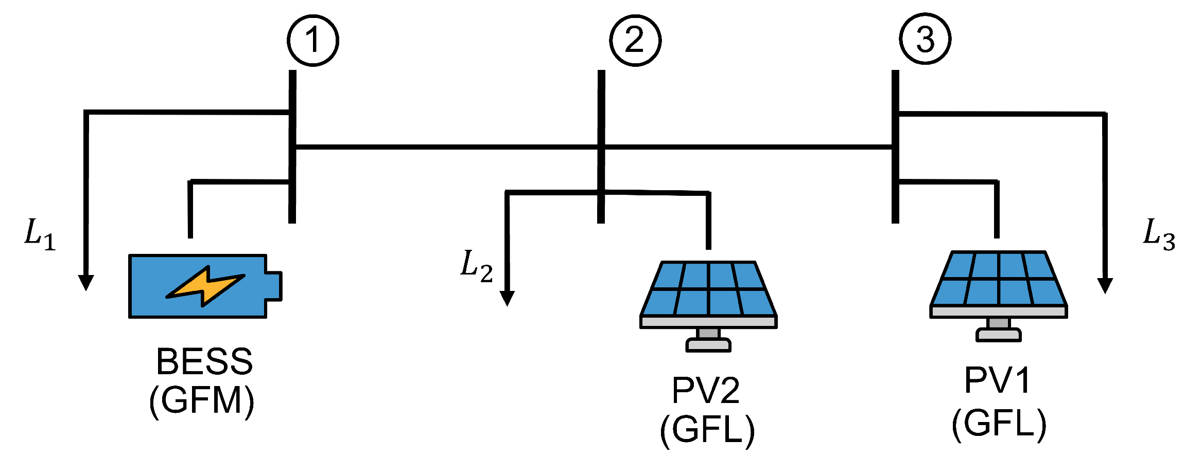
Figure 3.
QSTS PF simulation results for Scenario III: active power, BESS SoC, and frequency.
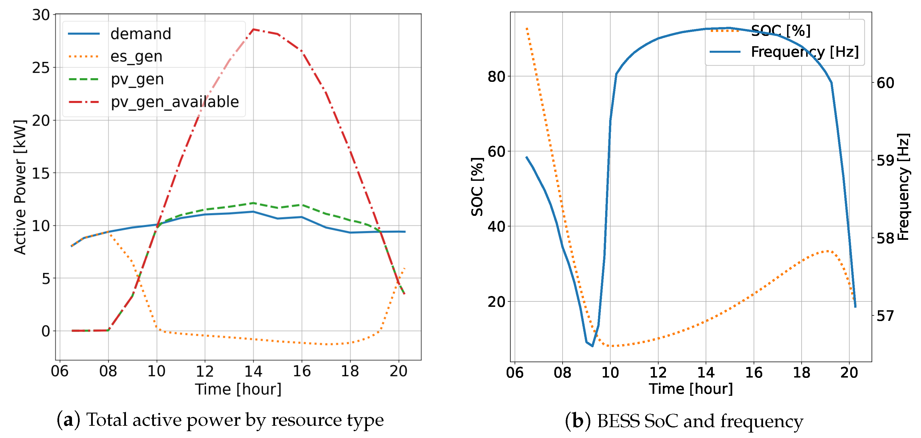
Figure 4.
QSTS PF simulation results for Scenario III: bus voltages and reactive power.
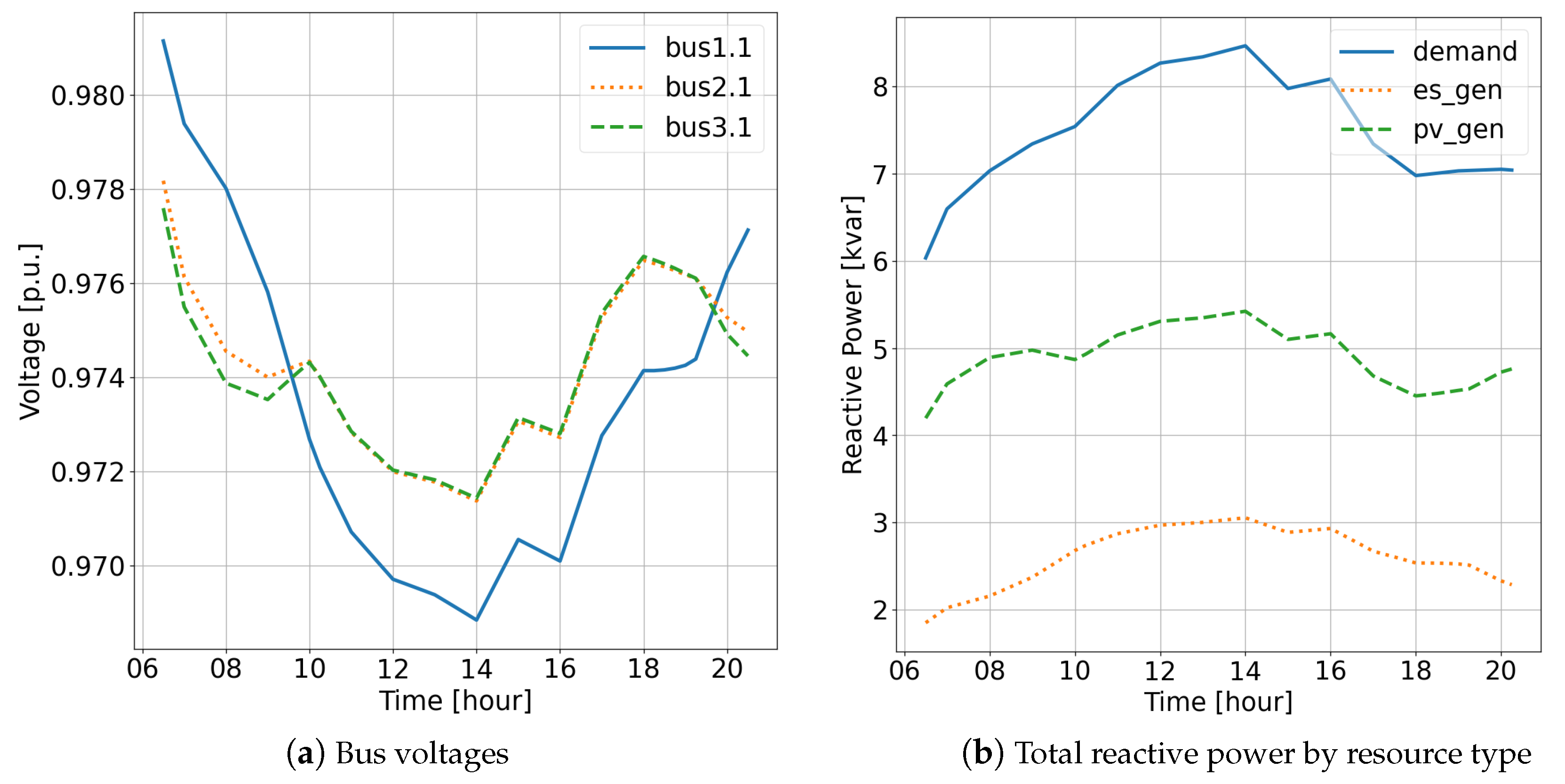
Figure 5.
QSTS OPF simulation results for Scenario III: active power, BESS SoC, and frequency.
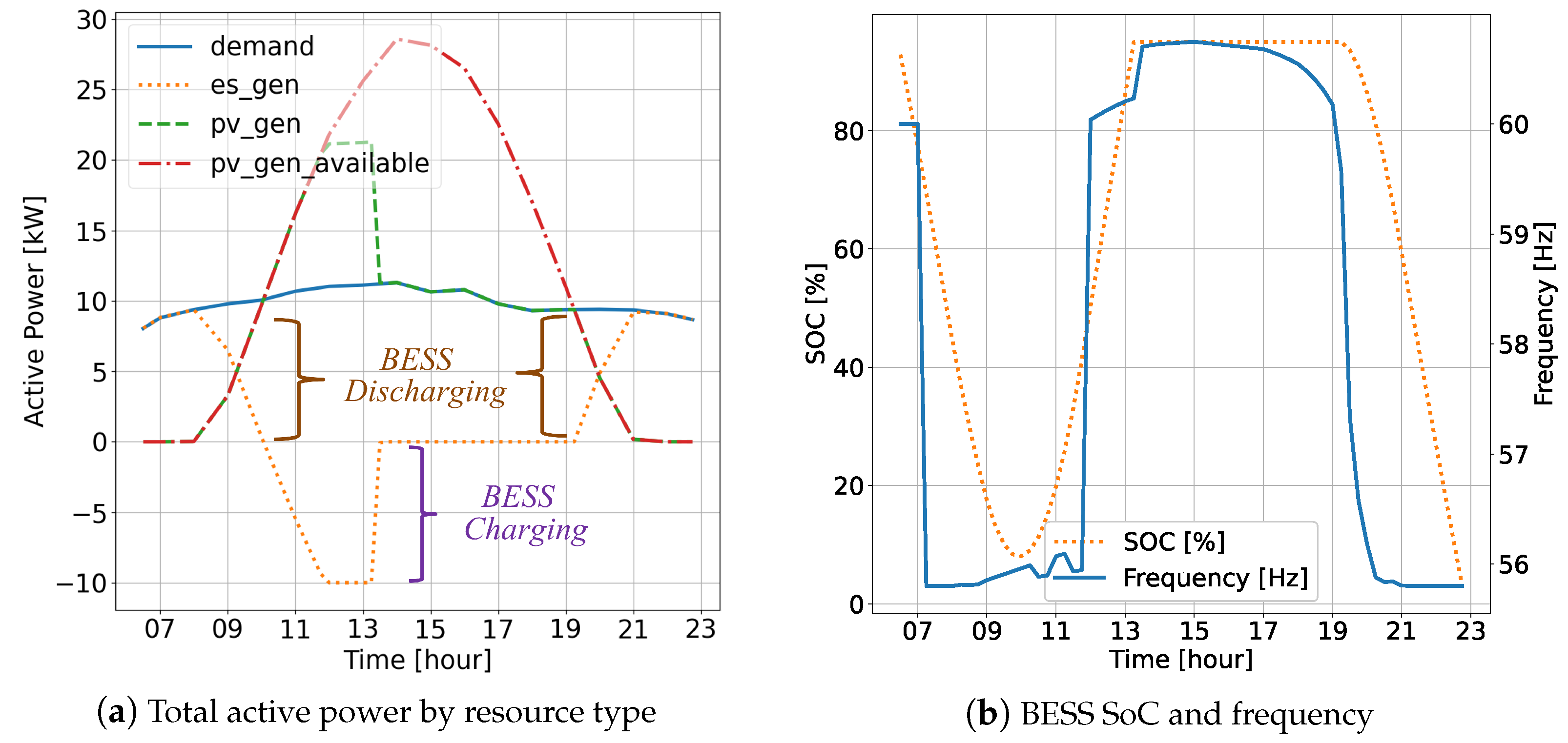
Figure 6.
QSTS OPF simulation results for Scenario III: bus voltages and reactive power.
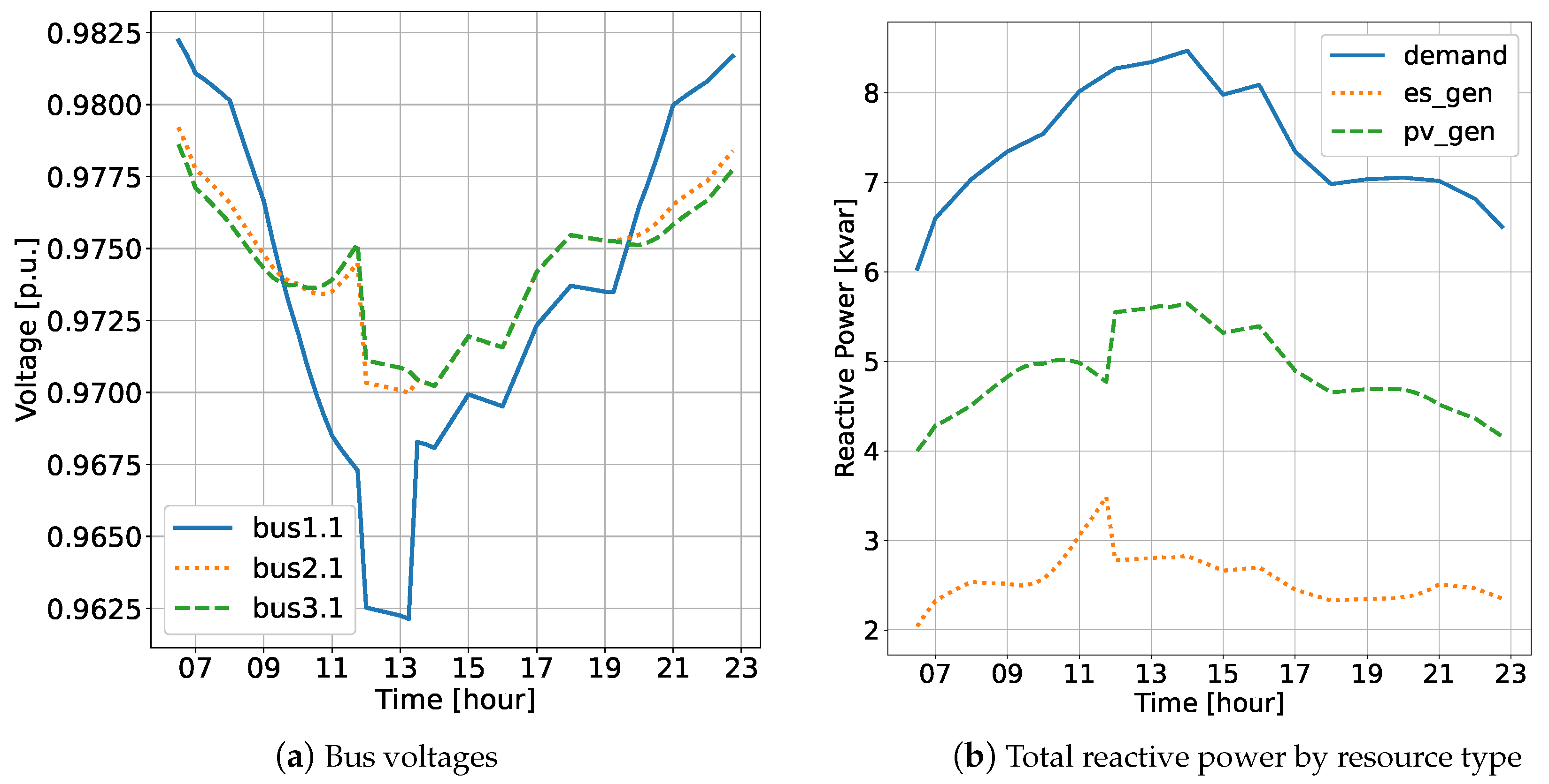
Figure 7.
Islanded microgrid of modified IEEE four-bus system.

Figure 8.
QSTS PF simulation results of a three-phase islanded microgrid: active power, BESS SoC, and frequency.
Figure 8.
QSTS PF simulation results of a three-phase islanded microgrid: active power, BESS SoC, and frequency.
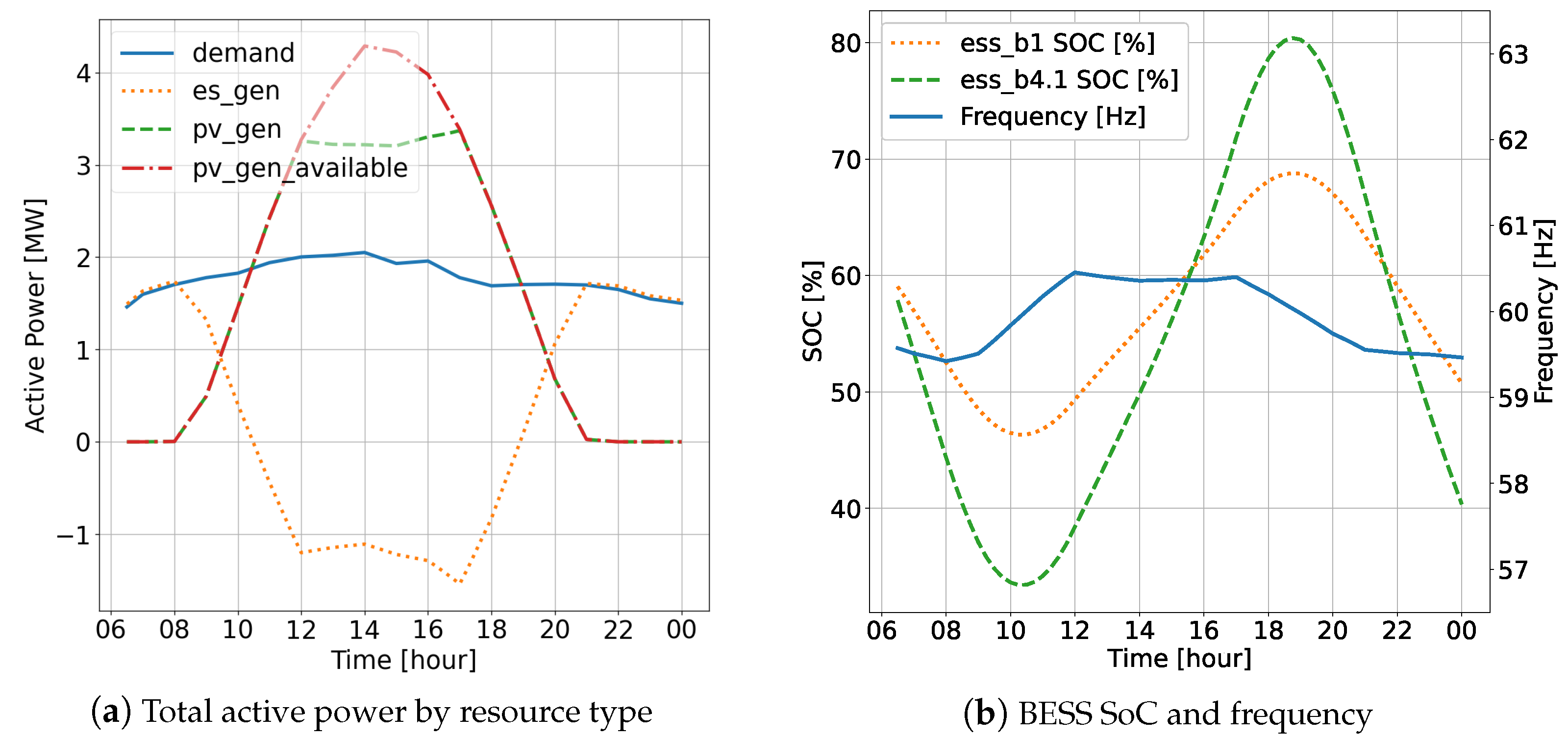
Figure 9.
QSTS PF simulation results of a three-phase islanded microgrid: bus voltage and negative sequence voltage.
Figure 9.
QSTS PF simulation results of a three-phase islanded microgrid: bus voltage and negative sequence voltage.
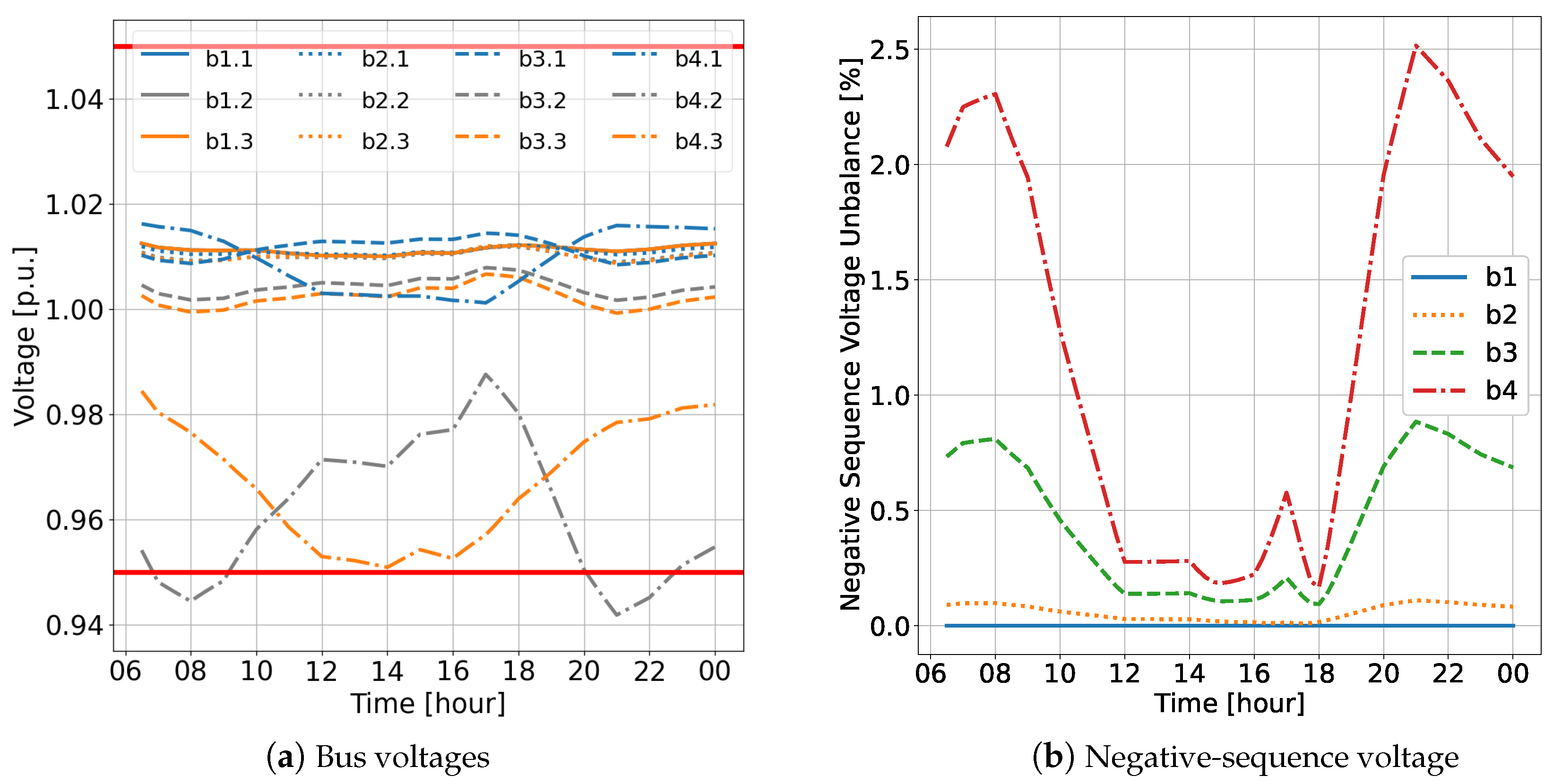
Figure 10.
QSTS OPF simulation results for a three-phase islanded microgrid: active power, BESS SoC, and frequency.
Figure 10.
QSTS OPF simulation results for a three-phase islanded microgrid: active power, BESS SoC, and frequency.
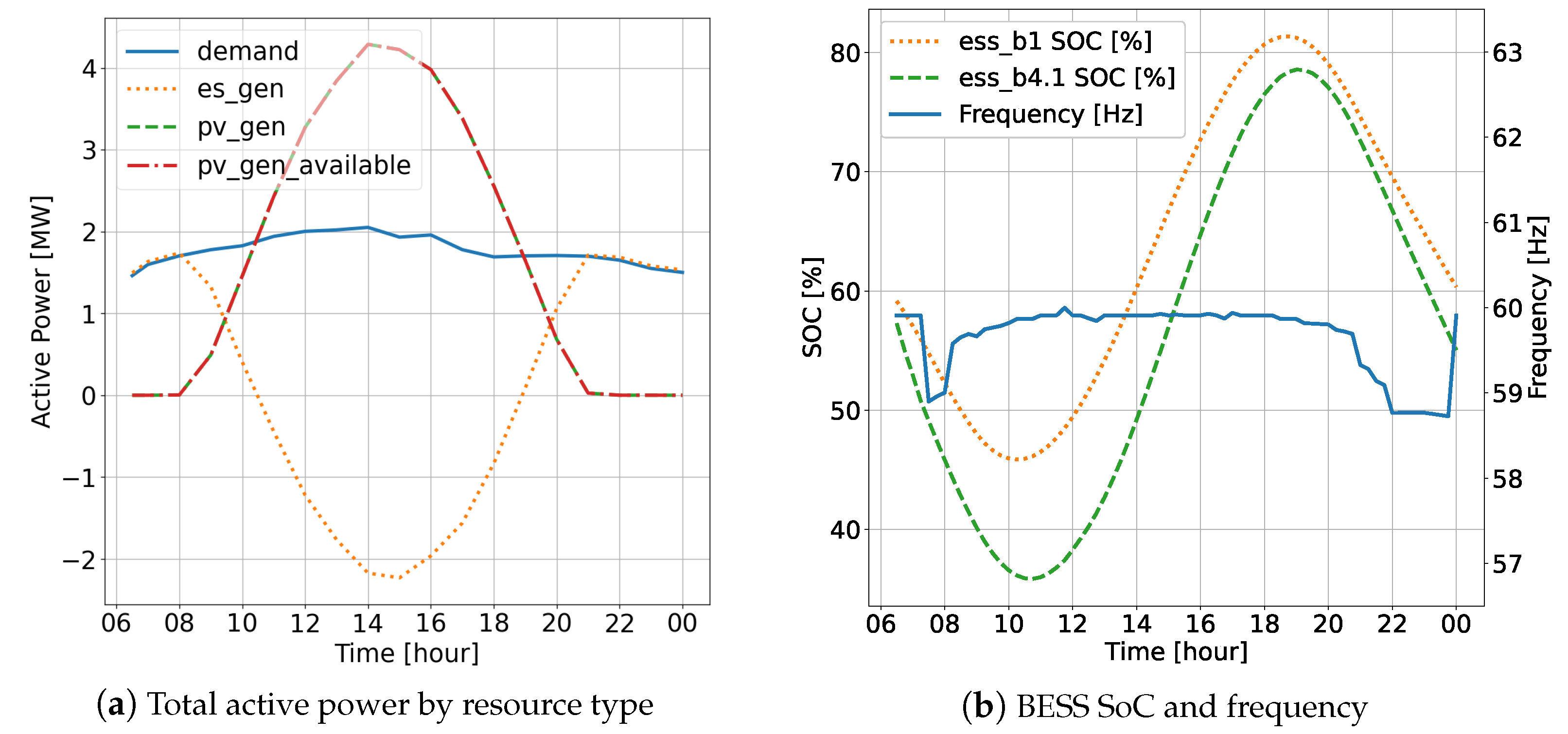
Figure 11.
QSTS OPF simulation results for a three-phase islanded microgrid: bus voltage and negative sequence voltage.
Figure 11.
QSTS OPF simulation results for a three-phase islanded microgrid: bus voltage and negative sequence voltage.


Table 1.
Sets and indices.
| Symbol | Description |
|---|---|
| Set of electric nodes | |
| Set of all PDEs | |
| Set of all electrical demand | |
| Set of non-controllable generators | |
| Set of controllable GFM s and the GFM which provides angle reference to the microgrid | |
| Set of controllable GFLs | |
| Set of GFM and GFL BESSs, | |
| , , , | Sets of electric nodes to which GFM s, GFL k, PDE l, and BESS e are connected |
Table 2.
Data and parameters.
| Parameters | Description |
|---|---|
| , | Conductance and susceptance between nodes i and j (S), respectively |
| , | Conductance and susceptance of PDE l between nodes i and j, respectively, where i, j ∈ (S) |
| System frequency setpoint for droop control (rad/s) | |
| , | Profile of available active power capacities such as SoC or irradiance of GFM s or GFL k (p.u.) |
| , , , | Droop coefficients of GFM s or GFL k, respectively (rad/(s·W), V/var) |
| , | Droop control voltage setpoints of GFM s or GFL k, respectively (V) |
| , | Active and reactive power demand d at node i, respectively (W, var) |
| , | Active and reactive power generation of non-controllable generator u at node i, respectively (W, var) |
| T | OPF planning horizon (h) |
| Initial SoC level of BESS e (p.u.) | |
| , | Lower and upper limits of SoC level of BESS e, respectively (p.u.) |
| , | Upper apparent power limits of GFM s or GFL k, respectively (VA) |
| Energy rating of ESS e (kWh) | |
| , | Lower and upper voltage limits at node i, respectively (V) |
| , | Lower and upper frequency limits, respectively (rad/s) |
| Upper current limit of PDE l (A) | |
| Target SoC level of ESS e (p.u.) | |
| , , , | Target active and reactive power dispatches of GFM s or GFL k (W or var) |
| Cost or penalty of operating BESS e at a mismatched SoC level rather than the target level (USD) | |
| , , , | Cost or penalty of operating GFM s or GFL k at mismatched power levels (USD/VA2) |
Table 3.
Variables.
| Variable | Description |
|---|---|
| System frequency (rad/s) | |
| , | Voltage magnitude and phase angle of node , respectively (V, rad) |
| , | Active and reactive power injection per phase of GFM s at node , respectively (W, var) |
| , | Active and reactive power injection per phase of GFL k to node , respectively (W, var) |
| , | Total active and reactive power injection of GFL k, respectively, calculated according to droop control (W, var) |
| , | Active and reactive power injection setpoints of GFM s, respectively (W, var) |
| , | Active and reactive power injection setpoints of GFL k, respectively (W, var) |
| , | Positive sequence voltage magnitude and phase angle of GFM s, respectively (V, rad) |
| , , | Real and imaginary components and magnitude of the positive sequence voltage of GFL k (V) |
| , | Real and imaginary components of the current injection of PDE l to the node , respectively (A) |
| SoC level of ESS e at the end of the OPF planning horizon (p.u.) |
Table 4.
Details of the IBRs and loads in the three-bus microgrid.
| Circuit Components | Specifications |
|---|---|
| BESS | Rating: 10 kW, 14 kVA, 28 kWh |
| , : 0.754 rad/(s·kW) and 2.45 V/kvar | |
| Initial SoC: 100% | |
| Inverter Type: GFM | |
| PV 1 | Rating: 10 kW, 14 kVA |
| , : 0.754 rad/(s·kW) and 2.45 V/kvar | |
| Inverter Type: GFL | |
| PV2 | Rating: 20 kW, 22 kVA |
| , : 0.377 rad/(s·kW) and 2.62 V/kvar | |
| Inverter Type: GFL | |
| Loads | kVA |
Table 5.
A summary of the details of the study cases in Scenario I: the active and reactive power setpoints and consideration of the kW and kVA limits of PV1.
Table 5.
A summary of the details of the study cases in Scenario I: the active and reactive power setpoints and consideration of the kW and kVA limits of PV1.
| Case | (kW) | (kvar) | kW Limit | kVA Limit | Constraints |
|---|---|---|---|---|---|
| 1.1 | 10 | 0 | ✗ | ✗ | Equations (1)–(4), (7), (15), (16), (35), and (39)–(41) |
| 1.2 | 10 | 0 | ✓ | ✗ | Equations (1)–(4), (7), (16), (18), (20), (35), and (39)–(41) |
| 1.3 | 10 | 10 | ✓ | ✓ | Equations
(1)–(4), (7), (18)–(21), (35), and (39)–(41) |
Table 6.
Table summarizing power flow results in Scenario I, including active and reactive power generation of BESS and PV1 (, , , ), voltage magnitudes at buses 1, 2, and 3 (, , ), BESS state of charge after 15 min (), and system frequency (f).
Table 6.
Table summarizing power flow results in Scenario I, including active and reactive power generation of BESS and PV1 (, , , ), voltage magnitudes at buses 1, 2, and 3 (, , ), BESS state of charge after 15 min (), and system frequency (f).
| Case | (kW) | (kvar) | (kW) | (kvar) | (p.u.) | (p.u.) | (p.u.) | (%) | f (Hz) |
|---|---|---|---|---|---|---|---|---|---|
| 1.1 | 2.51 | 5.77 | 12.51 | 5.49 | 0.9411 | 0.9420 | 0.9440 | 97.76 | 59.6987 |
| 1.2 | 5.01 | 5.67 | 10.00 | 5.59 | 0.9422 | 0.9416 | 0.9430 | 95.53 | 59.3988 |
| 1.3 | 5.02 | 1.46 | 10.00 | 9.80 | 0.9851 | 0.9857 | 0.9875 | 95.52 | 59.3980 |
Table 7.
Table summarizing percentage difference errors in power flow results for Scenario I. A comparison is made between the proposed and referenced modeling approaches for active and reactive power generation of BESS and PV1 (, , , ), voltage magnitudes at buses 1, 2, and 3 (, , ), BESS state of charge after 15 min (), and system frequency (f).
| Case | f | ||||||||
|---|---|---|---|---|---|---|---|---|---|
| 1.1 | 0.001 | 0.009 | 0.004 | −0.017 | 0.000 | 0.000 | 0.011 | 0.000 | 0.000 |
| 1.2 | 0.023 | 0.001 | −0.011 | −0.001 | 0.000 | 0.000 | 0.000 | −0.001 | −0.001 |
| 1.3 | 0.000 | 0.004 | 0.000 | −0.001 | −0.010 | −0.010 | −0.010 | 0.000 | −0.002 |
Table 8.
A summary of the details of the study cases in Scenario II, with the active and reactive power setpoints of the BESS and the initial SoC level.
Table 8.
A summary of the details of the study cases in Scenario II, with the active and reactive power setpoints of the BESS and the initial SoC level.
| Case | (kW) | (kvar) | Initial SoC (%) |
|---|---|---|---|
| 2.1 | 0 | 0 | 100 |
| 2.2 | 0 | 0 | 5 |
| 2.3 | 0 | 0 | 3 |
| 2.4 | 5 | 0 | 100 |
| 2.5 | 0 | 13 | 100 |
Table 9.
Table summarizing power flow results in Scenario II, including active and reactive power generation of BESS and PV1 (, , , ), voltage magnitudes at buses 1, 2, and 3 (, , ), BESS state of charge after 15 min (), and system frequency (f).
Table 9.
Table summarizing power flow results in Scenario II, including active and reactive power generation of BESS and PV1 (, , , ), voltage magnitudes at buses 1, 2, and 3 (, , ), BESS state of charge after 15 min (), and system frequency (f).
| Case | (kW) | (kvar) | (kW) | (kvar) | (p.u.) | (p.u.) | (p.u.) | (%) | f (Hz) |
|---|---|---|---|---|---|---|---|---|---|
| 2.1 | 7.50 | 5.57 | 7.50 | 5.68 | 0.9432 | 0.9412 | 0.9420 | 93.30 | 59.0995 |
| 2.2 | 5.01 | 5.67 | 10.00 | 5.59 | 0.9422 | 0.9416 | 0.9430 | 0.53 | 47.9777 |
| 2.3 | 5.01 | 5.67 | 10.00 | 5.59 | 0.9422 | 0.9416 | 0.9430 | −1.47 | 39.9628 |
| 2.4 | 10.01 | 5.47 | 5.01 | 5.79 | 0.9441 | 0.9407 | 0.9410 | 91.06 | 59.3989 |
| 2.5 | 7.52 | 11.96 | 7.52 | −0.69 | 1.0106 | 1.0070 | 1.0071 | 93.28 | 59.0973 |
Table 10.
Table summarizing percentage difference errors in power flow results for Scenario II. A comparison is made between the proposed and referenced modeling approaches for active and reactive power generation of BESS and PV1 (, , , ), voltage magnitudes at buses 1, 2, and 3 (, , ), BESS state of charge after 15 min (), and system frequency (f).
| Case | f | ||||||||
|---|---|---|---|---|---|---|---|---|---|
| 2.1 | 0.000 | 0.004 | 0.001 | −0.004 | 0.000 | 0.000 | 0.000 | 0.000 | 0.000 |
| 2.2 | 0.003 | 0.006 | 0.000 | 0.179 | 0.000 | 0.000 | 0.000 | −0.025 | −0.001 |
| 2.3 | 0.003 | 0.026 | 0.000 | −0.025 | 0.000 | 0.000 | 0.000 | 0.006 | −0.001 |
| 2.4 | 0.000 | −0.003 | 0.001 | 0.003 | 0.000 | 0.000 | 0.000 | 0.000 | 0.000 |
| 2.5 | 0.002 | −0.033 | 0.003 | 0.000 | 0.000 | 0.000 | 0.000 | 0.000 | 0.000 |
Table 11.
Table summarizing the IBR specifications in Demonstration II.
| Circuit Components | Specifications |
|---|---|
| BESS_1 | Rating: 10 MW, 7 MVA, 28 MWh |
| , : 1.508 rad/(s·MW) and 146.96 V/Mvar | |
| Initial SoC: 60% | |
| Inverter Type: GFM | |
| Location: Phase A, B, C of Bus 1 | |
| PV_1 | Rating: 4.5 MW, 5 MVA |
| , : 1.676 rad/(s·MW) and 110.20 V/Mvar | |
| Inverter Type: GFL | |
| Location: Phase A, B, C of Bus 4 | |
| BESS_2 | Rating: 2 MW, 2.5 MVA, 5 MWh |
| , : 3.770 rad/(s·MW) and 160.12 V/Mvar | |
| Initial SoC: 60% | |
| Inverter Type: GFL | |
| Location: Phase A of Bus 1 |
Disclaimer/Publisher’s Note: The statements, opinions and data contained in all publications are solely those of the individual author(s) and contributor(s) and not of MDPI and/or the editor(s). MDPI and/or the editor(s) disclaim responsibility for any injury to people or property resulting from any ideas, methods, instructions or products referred to in the content. |
© 2023 by the authors. Licensee MDPI, Basel, Switzerland. This article is an open access article distributed under the terms and conditions of the Creative Commons Attribution (CC BY) license (https://creativecommons.org/licenses/by/4.0/).
Share and Cite
MDPI and ACS Style
Siratarnsophon, P.; Kim, W.; Barry, N.; Chatterjee, D.; Santoso, S. Optimal Power Flow for Unbalanced Three-Phase Microgrids Using an Interior Point Optimizer. Energies 2024, 17, 32. https://doi.org/10.3390/en17010032
AMA Style
Siratarnsophon P, Kim W, Barry N, Chatterjee D, Santoso S. Optimal Power Flow for Unbalanced Three-Phase Microgrids Using an Interior Point Optimizer. Energies. 2024; 17(1):32. https://doi.org/10.3390/en17010032
Chicago/Turabian StyleSiratarnsophon, Piyapath, Woosung Kim, Nicholas Barry, Debjyoti Chatterjee, and Surya Santoso. 2024. "Optimal Power Flow for Unbalanced Three-Phase Microgrids Using an Interior Point Optimizer" Energies 17, no. 1: 32. https://doi.org/10.3390/en17010032
Note that from the first issue of 2016, this journal uses article numbers instead of page numbers. See further details here.