Remaining Useful Life Prediction of Electromagnetic Release Based on Whale Optimization Algorithm—Particle Filtering

Abstract

The DC circuit breaker is a crucial equipment for eliminating faults in DC transmission lines. The electromagnetic release functions as a critical component that restricts the circuit breaker’s lifespan. It is essential to prioritize its safety and reliability during usage and predicting its remaining useful life (RUL) is paramount. This paper proposes a new prediction technique based on particle filtering (PF) and the whale optimization algorithm (WOA) for the remaining useful life of electromagnetic release. The particle filtering algorithm is a commonly used technique in practical engineering fields such as target tracking and RUL prediction. It is a mainstream method for solving the parameter estimation of non-linear non-Gaussian systems. The WOA is introduced to improve the PF algorithm in order to ensure the diversity of particles and lessen the effect of particle degradation. The WOA replaces the traditional resampling process, and after each computation is finished, the weights of the particles in the particle set are reassigned in order to improve the particle distribution and increase algorithm accuracy. The rate of loss of the spring reaction force and the striker counterforce are chosen as the degradation characteristics after the degradation factors of electromagnetic release are analyzed. The degradation curves at different temperatures of electromagnetic release are obtained using the accelerated life test, and the full-life data during normal operation are derived using the Arrhenius equation. Finally, the RUL is predicted by comparing this paper’s method with the conventional PF method. The experimental results demonstrate that the method presented in this paper can more accurately predict the RUL of the electromagnetic release and has a higher prediction accuracy.

1. Introduction

Short-circuit fault is one of the most frequent faults in the operation of electrical systems, and it is extremely unfavorable to the safe operation of power systems. In the initial stage of short circuit, the impedance at the short circuit point is very small, so it leads to an instantaneous rise in current, which will cause serious heating or even damage to the conductor and insulation. At the same time, the conductors of electrical equipment will be subjected to a great deal of electrodynamic force between the conductors, which may cause deformation of the conductors or coils so as to be damaged [1,2,3]. The electrical systems’ voltage will drop as a result of the short circuit, which will interfere with the user’s power equipment’s ability to function normally and eventually damage it. Therefore, analyzing its degradation law, predicting its RUL, and ensuring the reliability of electromagnetic release action can effectively reduce the occurrence of electrical accidents caused by the reduction in reliability of low-voltage circuit breakers. Electromagnetic release is an important component of low-voltage DC circuit breakers to complete the instantaneous breaking task when it passes the short-circuit current [4,5].

Many scholars have already carried out research work on the life prediction of circuit breakers. The authors of [6] established mathematical models of arc erosion factor in different current ranges and mathematical models of average contact quality loss rate and proposed a method for predicting the remaining useful electrical life of circuit breakers under different variable stress conditions. The authors of [7] proposed a life prediction method based on multi-feature fusion of electromechanical signals by the action process of energy storage operating mechanism. However, the above studies mainly focus on the electrical life of the circuit breaker and the operating mechanism, and few studies have been reported on the life prediction of electromagnetic release for circuit breakers. In addition, circuit breakers have a long service life and high reliability. Testing circuit breakers under normal operating conditions is too costly and time-consuming, and the available failure data are insufficient to create a useful performance degradation model that would enable life prediction. For this reason, lifetime data are primarily obtained through accelerated degradation test. The authors of [8] conducted a constant stress accelerated degradation test with temperature as the accelerating stress and residual action current value as the degradation eigenvalue and established a RUL prediction model based on the Wiener process after obtaining the degradation law of circuit breaker performance.

Particle filtering is a recursive filtering method based on Bayesian estimation and the Monte Carlo method. For the standard particle filtering algorithm, there will be a degradation of weights, which is manifested in the fact that after many times of recursion, only a small number of particles have larger weights, and the rest have almost zero weights. Weight degradation can be resolved by resampling, but doing so will also cause a phenomenon known as sample impoverishment, in which high weighted particles are overcopied and there are fewer effective particles overall, which lowers the particles’ information capacity. Numerous academics have conducted extensive research to address the aforementioned issues. The authors of [9] proposed a particle filtering method using genetic algorithm to adaptively optimize low-weighted particles, which effectively mitigates the problem of weight degradation and ensures particle diversity. The authors of [10] combined an improved artificial firefly algorithm and particle filtering, effectively improving the prediction accuracy. The authors of [11] proposed a grey wolf particle filtering, by simulating the four behavioral patterns in the hunting process of grey wolf packs to update the particle positions, improve the particle distribution, and increase the particle diversity. In 2016, Mirjalili and Lewis proposed a whale optimization algorithm based on the simulation of humpback whale population hunting behavior. In comparison to the above swarm intelligence optimization algorithms, the whale optimization algorithm can flexibly change the search strategy, by dynamically updating the weights of the population’s search and predation behaviors, so that it can conduct the fast global search for optimality at the early stage and the high-precision local search at the later stage.

Based on the problems mentioned above, this paper first obtains electromagnetic release performance degradation data through accelerated degradation test and develops a mathematical model to describe the degradation process of electromagnetic release, and then introduces the whale algorithm to optimize the resampling process of particle filtering, so that the particles are closer to the high likelihood region and their weights are more accurately and reasonably assayed. The WOA-PF algorithm and the PF algorithm are used to predict the lifetime, which is then compared with the real value. The optimized particle filtering algorithm improves particle degradation and particle tracking ability, making the prediction results more accurate.

2. Theoretical Foundation

2.1. Particle Filtering

PF is often used to solve filtering problems with non-linear state spaces, non-Gaussian noise distributions, and good robustness to noise [12,13,14].

The derivation of the PF algorithm first needs to establish the system model, including two parts, the state equation and the observation equation. The model expression is as follows:

$$\left\{\begin{array}{l}{x}_k=f\left(x_{k-1},v_{k-1}\right)\\ y_k=h\left(x_k,u_k\right)\end{array}\right.$$

(1)

where $f(•)$ denotes state relation function, $x_k$ is the system state variable of the system at moment k, and $v_{k-1}$ denotes the system state noise. $h(•)$ denotes the mapping function between observations and state values, $y_k$ denotes the observation variable of the system at the current moment, and $u_k$ denotes the system observation noise.

Particle filtering is performed by first sampling from a known and easily sampled reference distribution 𝑞(𝑋_0:𝑘|𝑌_1:𝑘), and approximating the a posteriori distribution by weighting and summing the set of particles obtained from the sampling of the reference distribution 𝑝(𝑋_0:𝑘|𝑌_1:𝑘), i.e.,

$$p\left(X_{0:k}\left|Y_{1:k}\right.\right)\approx {\displaystyle \sum _{i=1}^N{\tilde{w}}_k^i}\delta \left(x_{0:k}-x_{0:k}^i\right)$$

(2)

where $x_{0:k}=\{x_0, x_1, \dots , x_k\}$ is the state of the system from 0 to the moment of 𝑘, and {$x_{0:k}^i$, 𝑖 = 1,2, …, 𝑁} is the set of samples sampled from the probability density 𝑞(𝑋_0:𝑘) at the moment 𝑘, i.e., the sampled particles. $\{{\tilde{w}}_k^i,i=\mathrm{1,2},\dots ,\mathrm{N}\}$ are the corresponding normalised weights of the particles, and the weights are selected by the importance sampling method. The set of particles ${\left\{x_{0:k}^i\right\}}_{i=1}^N$ is obtained from the importance density function 𝑞(𝑋_0:𝑘|𝑌_1:𝑘), and the particle weights can be expressed as follows:

$$w_k^i\propto \frac{p\left(X_{0:k}^i\left|Y_{1:k}\right.\right)}{q\left(X_{0:k}^i\left|Y_{1:k}\right.\right)}$$

(3)

Because particle degradation may occur after PF continuous iterative operation, making particle weight distribution unreasonable, the traditional PF algorithm sets up a resampling process: resample the samples, keep the particles with large weights, discard the particles with small weights, and then redistribute the weights to update all the particles to be weighted as follows:

$$w_k^i=\frac{1}{N}$$

(4)

2.2. Whale Optimisation Algorithm

The whale optimization algorithm (WOA) is a new heuristic optimization algorithm proposed [15,16,17] that mimics the hunting behavior of humpback whales. In the whale optimization algorithm, each whale represents a solution, and the whales keep exploring and rounding up the prey in the algorithm’s iterative process and keep trying to improve their solutions. The whale optimization algorithm is capable of solving a wide range of complex optimization issues and has a fast convergence rate. Based on the typical hunting behavior of whales, the basic process of the whale optimization algorithm consists primarily of the following three steps:

• Initialization: determine the number of whale groups N, the maximum number of iterations m, and assign an initial position to each whale before generating the initial population.
• Search: Each whale explores the environment according to a set of rules. This process can be used to simulate whales encircling, chasing, and attacking their prey. When a whale moves, the fitness value for the current whale population is calculated. If the current fitness value is higher than the previous fitness value, it is chosen as the best solution.
• Update: The algorithm will update all whale positions and repeat the previous steps after all whales have completed moving and evaluating. Up until the predetermined accuracy or the maximum number of iterations are reached, several iterations are carried out.

3. Optimizing Particle Filtering Based on the Whale Optimization Algorithm

3.1. Design of the Fitness Function

When the particle degradation phenomenon occurs, the traditional particle filtering algorithm selects the resampling strategy, discarding the particles with small weights and copying the particles with large weights several times to increase the number of effective particles, so as to achieve the purpose of suppressing the degradation, but this also causes the particles to lose diversity after resampling, and the problem of sample exhaustion occurs, which eventually recurs [18].

The joint WOA-PF algorithm is obtained by combining the WOA and the PF algorithm, the core idea of which is to optimize the particles obtained from importance sampling by replacing the re-sampling phase of the basic PF with the whale’s predation process. Individual particles in the particle filter correspond to individual whales in the whale population, and based on the size calculated by the fitness function, the whales continuously search for prey and move towards whales with high fitness, searching for the most effective and optimal solution, similar to the process by which particles are improved to be more consistent with the true posterior distribution, increasing the number of effective particles and obviating the need for a particle filter.

When the whale optimization algorithm is introduced, although the whale will search for the optimal prey position through many iterations, thus improving the filtering efficiency of WOA-PF, when WOA is applied to the particle filtering non-linear non-Gaussian model, the computationally complex particle prediction accuracy decreases, and the probability of particle loss and other problems increases, so some improvements are made to the WOA, and the traditional PF algorithm chooses the a priori probability density for the importance probability density, but this method ignores the current moment observation value, reducing the algorithm’s accuracy. When establishing the relationship between the particle filtering algorithm’s weights $w_k^i$ and the whale optimization algorithm’s fitness function, refer to the weights $w_k^i$ formula and use the most recent moment observation value as feedback information to correct the current target prediction result. The fitness function of the whale optimization algorithm is set as follows:

$$Fit\left(i\right)=\exp \left[-\frac{1}{2R_k}{\left(y_k-{\widehat{y}}_{k,i}\right)}^2\right]$$

(5)

where R_k is the variance of the systematic observation noise u_k, y_k is the observed value at moment k, and ${\widehat{y}}_{k,i}$ is the predicted value corresponding to whale i.

The traditional particle filtering algorithm must compare the difference between all particles and the optimal particle, which is a time-consuming and computationally intensive process. The improved WOA-PF algorithm greatly reduces the algorithm’s computational effort, requiring only the square of the difference between the observed and predicted values of each particle at each iterative step. At the same time, including the most recent particle observation improves the accuracy of the target prediction at the current and next moments, effectively improving the system’s overall filtering accuracy.

3.2. Adaptive Mutation Mechanisms

The whale optimization algorithm employs a forced random walk mechanism, which improves the ability to jump out of the local optimum to some extent but does not completely eliminate the possibility of premature maturation. The variance ${\sigma }^2$ of the whale population fitness and the size of the current fitness optimum are used in this case to determine whether the algorithm falls into the local optimum. Where ${\sigma }^2$ represents the total variation in each individual’s fitness within the whale population, a smaller value indicates a higher degree of group aggregation and a lower degree of population diversity; a larger value of optimal fitness indicates a closer approximation to the true position, and vice versa, suggesting a larger deviation between the group and the true position. If the algorithm is judged to be trapped in a local optimum, ${\sigma }^2\le \delta$ (set the variance threshold), and the size of the current optimal fitness value does not reach the theoretical optimal value or the target accuracy. At this point, the iteration’s optimal whales are replicated T, and the replicated whales are subjected to Cauchy perturbation mutation operation with a given probability P, and the optimal individuals after mutation are subjected to a secondary optimization search. The Cauchy mutation formula is as follows:

$$X^i=X^0\left(1+\tan \left(\pi \left(u-0.5\right)\right)\right)$$

(6)

where $X^i$ represents the location of the mutated individual, $X^0$ represents the location of the particle with the current optimal fitness function value, and u represents a random number from 0 to 1. Cauchy mutation can improve the algorithm’s global search ability; if the best fitness value of the T individuals after mutation is greater than the best fitness value of the current population, the location of the best point after mutation is used to determine the optimal location of the current generation of whales into the next iteration. The adaptive mutation operation can quickly find the global optimal point while increasing population diversity.

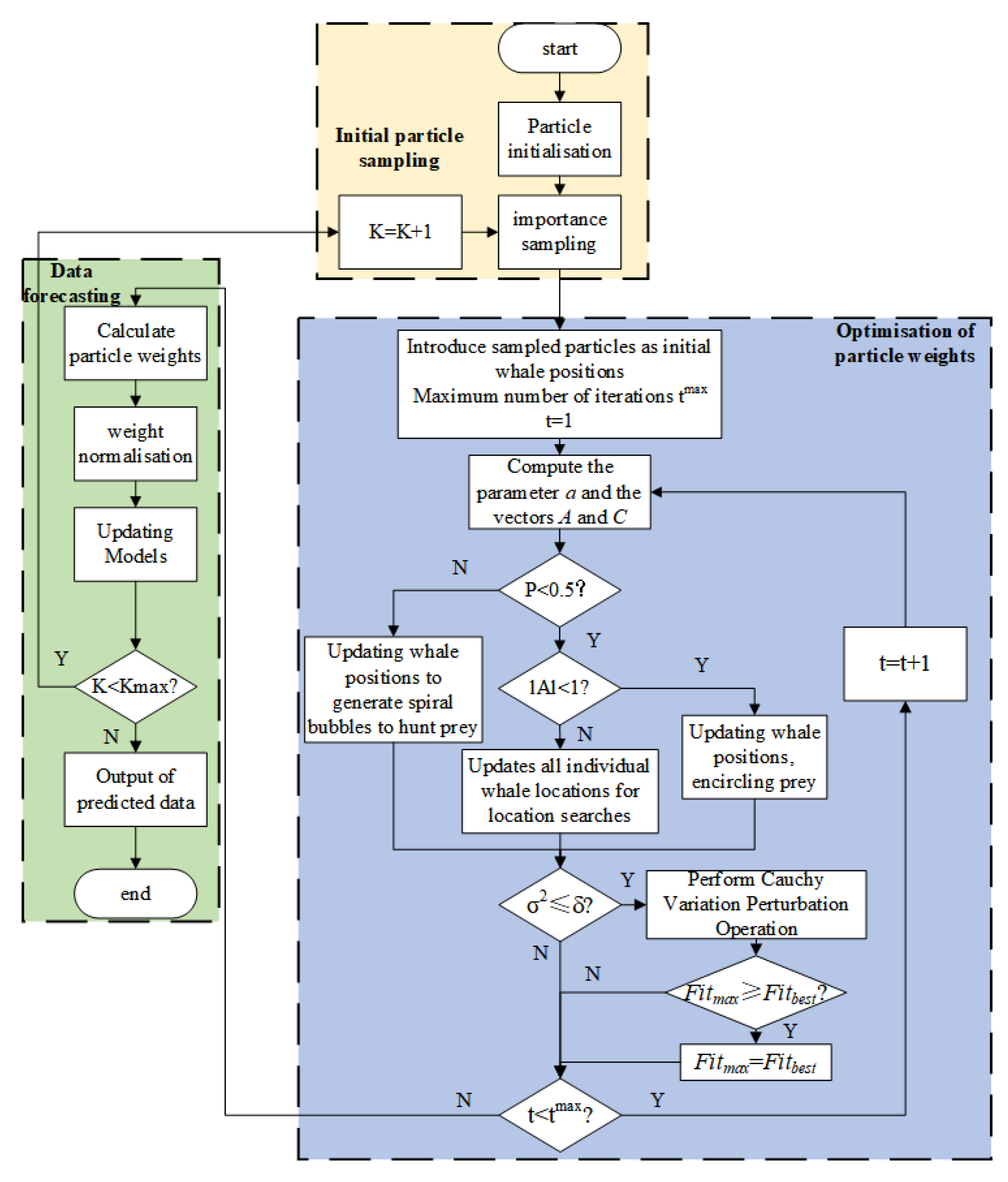
3.3. Algorithmic Step

The specific steps of the WOA-PF algorithm are as follows:

(1) Initialize the particle state with 𝑘 = 0, determine the parameter values, and sample from the previous distribution 𝑝(𝑋0) to derive the initialized state particle set $\left\{X_0^i,\mathrm{i}=\mathrm{1,2},\dots ,\mathrm{N}\right\}$ as the initial sample importance density function:

$$q\left(x_{0:k}\left|y_{1:k}\right.\right)=q\left(x_0\right){\displaystyle \prod _{j=1}^{k}q}\left(x_j\left|x_{0:j-1},y_{1:j}\right.\right)$$

(7)

(2) Importance sampling to obtain k particles and predict particle states, use Equation (1) to calculate particle state values and observations at the next moment, and use the particle state values as the initial positions of individual whales.

(3) Calculate the fitness of all whale positions based on the initially obtained positions of individual whales. Fit(i) using Equation (5) and sort them.

(4) Pre-iteration of the whale algorithm for the global search for optimal, randomly select an individual as a reference individual to update the whale position, i.e., create a random array to replace the whale position, forcing the whale to deviate from the optimal individual position, through which to find a more suitable prey, to strengthen the algorithm’s ability to explore, according to Equation (8), the simulation of the whale searching for prey to update the whale position.

$$X_k^{jnew}=X_k^{rand}-A_1\cdot D_k$$

(8)

$$D_k=\left|C_1\cdot X_k^{rand}-X_k^j\right|$$

(9)

where $X^{rand}$ is a randomly selected whale position vector. $X_k^{jnew}$ is the kth component of the spatial coordinate $X^{jnew}$. $X^j$ is the position of the individual whale.

$$C_1=2r_2$$

(10)

$$A_1=2a\cdot r_1-a$$

(11)

where $r_1,r_2$ are random numbers from 0 to 1, $a$ decreases linearly from 2 to 0 with the number of iterations, and the expression is as follows:

$$a=2-\frac{2t}{T_{\max }}$$

(12)

where t denotes the current number of iteration and $T_{max}$ is the maximum number of iterations.

(5) To determine whether each whale is feeding on the prey, the whale swims to the prey in a spiral motion while also contracting the encirclement circle, and the whale’s behavior of searching for encircling prey and spiral feeding on prey are synchronous and alternating according to Equation (13) to update the whale’s position and generate spiral bubbles to feed on the prey.

$$\left\{\begin{array}{l}{X}_k^{jnew}=X_k^{*}+D_k\cdot e^{bl}\cdot \cos \left(2\pi l\right),P\ge P_i\\ X_k^{jnew}=X_k^{*}-AD,\hspace{1em}\hspace{1em}\hspace{1em}\hspace{1em}\hspace{1em}P<P_i\end{array}\right.$$

(13)

where $b$ is a logarithmic spiral shape constant, $l$ is a random number from −1 to 1, $D_k=\left|X_k^{*}-X_k^j\right|$ is the distance between each current individual and the optimal individual, P is a random number from 0 to 1, and P_i is generally taken as 0.5.

(6) After many iterations, multiple better values are searched, and it should be determined whether to perform local search, i.e., as the number of iterations increases until |A| < 1, local search is performed, and the optimal individual is used as the reference individual, so that the whale population continues to approach the direction of the prey. To encircle the prey, the whale’s position is updated using Equation (14).

$$X_k^{jnew}=X_k^{*}-A_1\cdot D_k$$

(14)

$$D_k=\left|C_1\cdot X_k^{*}-X_k^j\right|$$

(15)

where $X^{*}$ is the position of the best individual whale.

(7) Determine the individual fitness value Fit(i), the optimal value Fit_max, the population mean fitness value Fit_mean, and the particle population fitness variance ${\sigma }^2$.

$$Fi{t}_{mean}=\frac{1}{N}{\displaystyle \sum _{i=1}^{N}Fit\left(i\right)}$$

(16)

$${\sigma }^2=\frac{1}{N-1}{\left(Fit\left(i\right)-Fi{t}_{mean}\right)}^2$$

(17)

If ${\sigma }^2\le \delta$ (the set variance threshold) and the current best fitness value are less than the theoretical maximum or the target accuracy, the algorithm is judged to be in a local optimum. If the random number distributed between 0 and 1 is less than the variance probability P, then the copied individuals are subjected to Cauchy variance perturbation operation to update their positions, as shown in Equation (6).

(8) Calculate the fitness value of the mutated individual and keep the particle with the highest fitness and its position. If the maximum fitness after mutation ${Fit}_{max}\ge {Fit}_{best}$, then update the value of the best fitness:

$$Fi{t}_{best}=Fi{t}_{\max }$$

(18)

(9) Determine if the maximum number of iterations T_max has been reached, and if so, go to Step (10), otherwise repeat Steps (3) to (8).

(10) The optimized whale positions are used as particles, and the population of particles from the previous iteration is kept, and the respective weights are calculated using Equation (3) and normalized using the following equation:

$${\omega }_k^i=\frac{{\omega }_k^i}{{\displaystyle \sum _{i=1}^N{\omega }_k^i}}$$

(19)

(11) Determine whether the total time step K_max has been reached or not, and if not return to Step (1) until the estimation is completed for all moments.

In summary, the flow of the WOA-PF algorithm is shown in Figure 1.

4. Experimental Verification

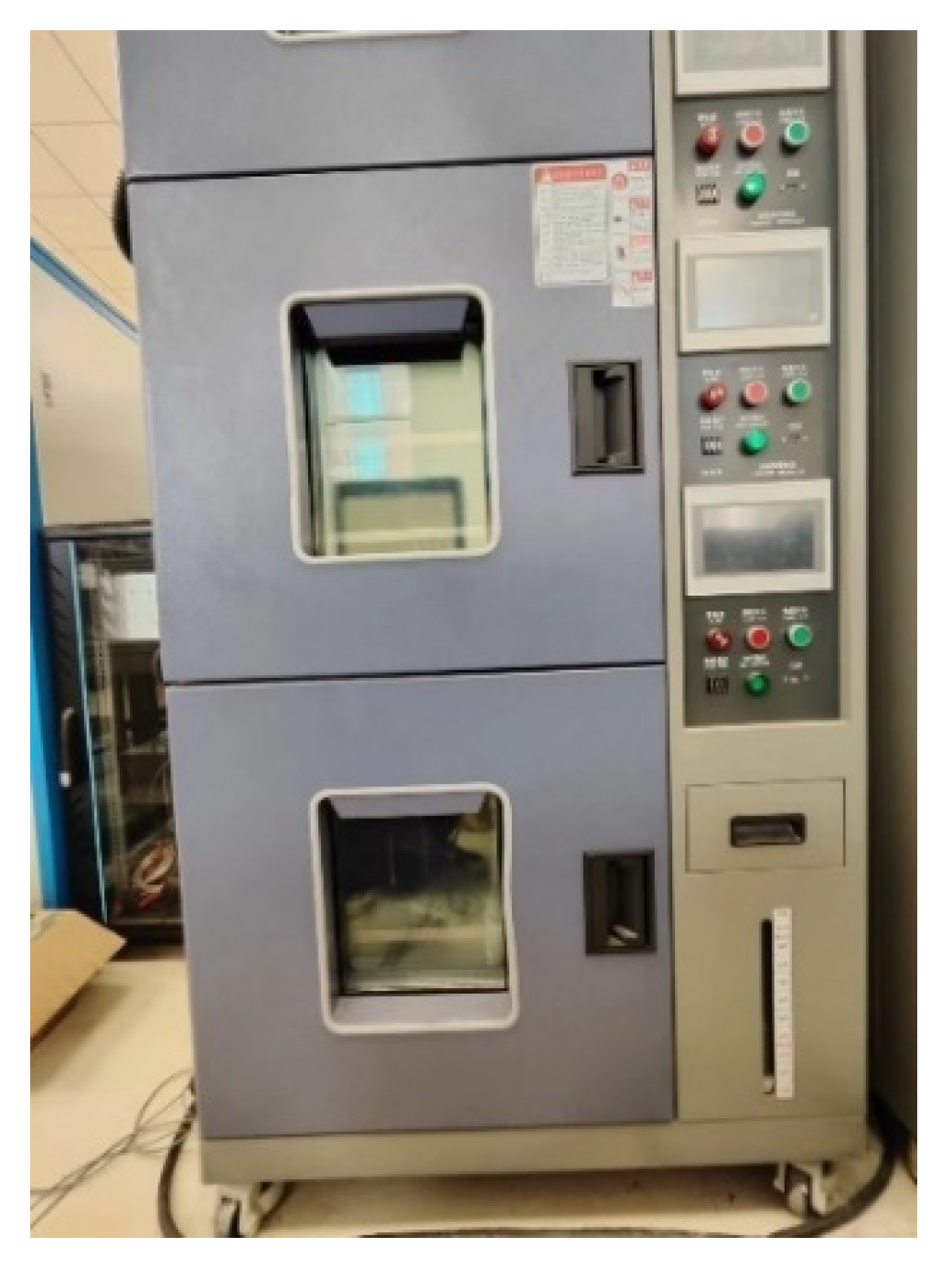
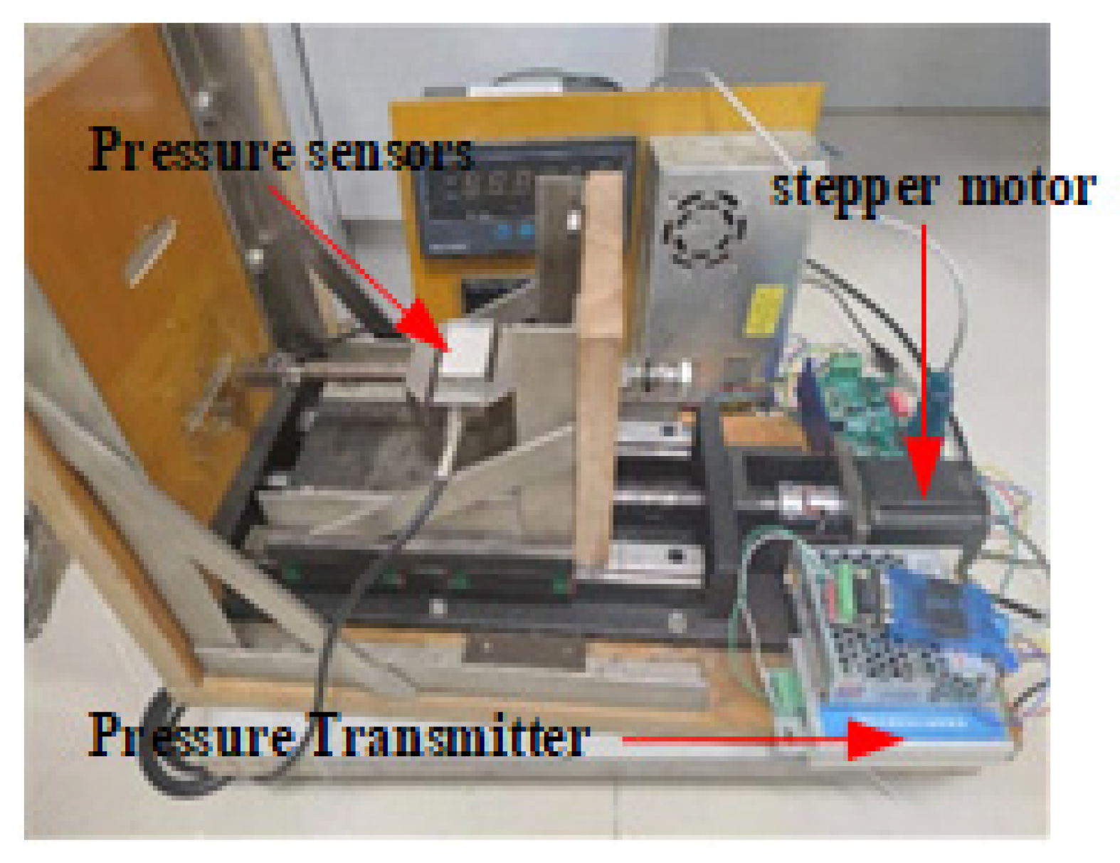
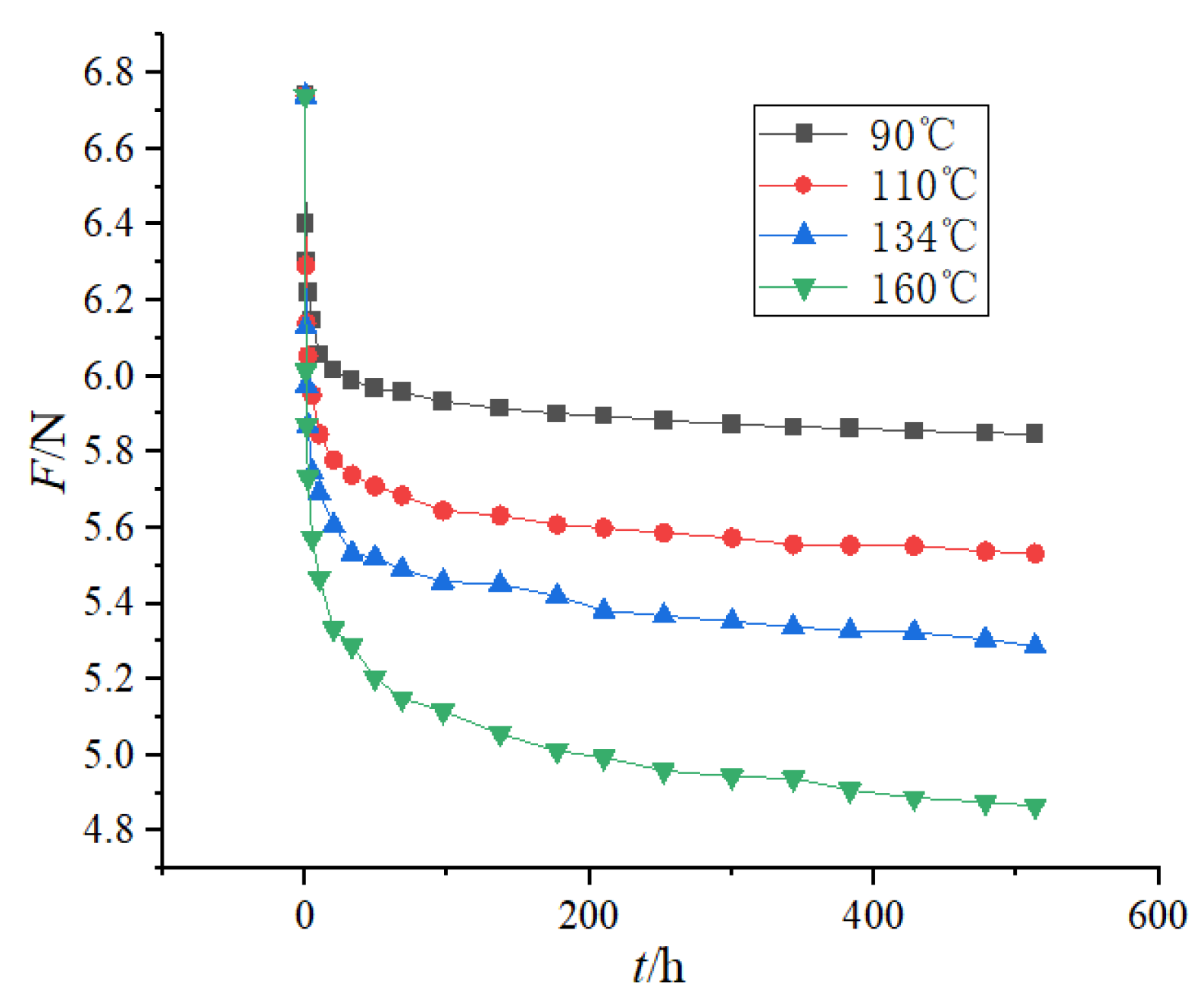
4.1. Experimental Programme and Analysis of Experimental Data

The electromagnetic release’s main structure consists of a moving iron core, a static iron core, a reaction spring, an electromagnetic coil, a yoke iron, a guide sleeve, and other components. The number of electromagnetic release actions is relatively small during the service period, and the performance degradation of the armature and yoke iron is relatively slow, so the performance degradation of the armature, yoke iron, and current conductor in the electromagnetic release can be ignored. As a result, the main factors influencing electromagnetic release performance degradation are the change of the reaction spring and the striker counterforce.

Because of the spring’s long life, short-term degradation under natural conditions is not obvious, so this paper uses an accelerated test to obtain the full life of the electromagnetic release, with the electromagnetic release position adjacent to the thermal release. In normal operation, the temperature around the electromagnetic release is very high, and the number of actions is small; therefore, temperature was chosen as the accelerating stress based on the above analysis. As shown in Figure 2, the main test equipment for the accelerated stress temperature test is a constant temperature test chamber. The force transducer equipment measures the spring reaction force and the striker counterforce, and the measured reaction force is the sum of the spring reaction force and the release reaction force when the moving core just touches the release lever, as shown in Figure 3. According to the Chinese national standard, when the sum of the spring reaction force and the striker counterforce is less than 80% of the electromagnetic suction force at the short-circuit setting current, the electromagnetic release is considered to have reached its failure threshold, and the electromagnetic release will operate incorrectly, and the electromagnetic release’s life will be terminated [19].

Degradation experiments on the electromagnetic release were carried out at four temperature points, 90 °C, 110 °C, 134 °C, and 160 °C, and the curve of the data of the total reaction force with time is shown in Figure 4. The degradation curve of the reaction force at various temperatures is shown in the figure to be primarily divided into two stages: as time passes, the degradation rate slows down to enter the second stage, which lasts for a long time, and the degradation gradually tends to stabilize. The slope of the curve in the first stage is very large, indicating that the degradation rate is faster at this time, and the duration is very short. The degree of degradation is also positively correlated with the temperature.

Since the degradation data obtained are non-linear with respect to time, which is not favorable for curve fitting and prediction of life, the curve was processed using the logarithm of time as the horizontal coordinate and the rate of loss of reaction force as the vertical coordinate to obtain the curve shown in Figure 5, where the rate of loss of reaction force is defined as follows:

$$\delta =\frac{F_0-F_t}{F_0}\times 100\%$$

(20)

where $\delta$ is the rate of loss of reaction force, F₀ is the initial reaction force in N, and F_t is the reaction force in N after the test.

From the figure, it can be seen that the rate of loss of the reaction force is linearly related to the logarithm of time, and the performance degradation process can be expressed as follows:

$$\delta =a\ln \left(t\right)+b$$

(21)

where a is the degradation rate and b is the model constant of the degradation process. The parameter estimates of the degradation trajectory model at different temperatures were estimated using Equation (21) and the results are shown in

Table 1. Model parameters at different temperatures.

Test Temperature/°C	$\widehat{\mathit{a}}$	$\widehat{\mathit{b}}$	Correlation Coefficient r
90	0.01083	0.06832	0.96630
110	0.01484	0.09066	0.97549
134	0.01621	0.11483	0.98331
160	0.02389	0.13154	0.99643

.

Assuming that the significance level is 0.01, after checking the table, we can obtain r_0.01 = 0.8340. The correlation coefficients in the table are all greater than 0.8340, so it can be assumed that the effect of linear regression is significant.

Since the thermal stress is used as the accelerating stress in this paper, and the main degradation factor spring is considered to satisfy the Arrhenius model, the Arrhenius model is chosen as the accelerating model, i.e.,

$$a=A\exp \left(-\frac{E_a}{kT}\right)$$

(22)

where $a$ is the rate of degradation, A is the Arrhenius constant, E_a is the activation energy, k is the Boltzmann constant, and T is the absolute temperature.

Taking logarithms on both sides of the above equation yields:

$$\ln a=\ln A-\frac{E_a}{k}\cdot \frac{1}{T}$$

(23)

Based on the data in the table, the linear relationship between the logarithm of the degradation rate and the inverse of the temperature was obtained using Equation (23), and the acceleration equation for the degradation rate of the performance parameter was obtained after linear fitting.

$$a=\exp \left(0.03673-1721.35/T\right)$$

(24)

The b in Equation (21) can be viewed as the amount of degradation after 1 h of degradation, which is obtained according to the Arrhenius equation:

$$b={\displaystyle {\int }_0^{1}A\exp \left(-\frac{E_a}{kT}\right)}dt=A\exp \left(-\frac{E_a}{kT}\right)$$

(25)

Again, using the data in the table, it was obtained using curve fitting:

$$b=\exp \left(1.42025-1476.78/T\right)$$

(26)

The surrounding temperature of the circuit breaker is T₀ = 75 °C when it operates normally because the electromagnetic release’s working position is near the thermal release. The electromagnetic release’s performance parameters at normal working temperature T₀ can be calculated, and Figure 6 displays the electromagnetic release’s performance degradation curve as a result.

$$\delta =0.0073906\ln t+0.059514$$

(27)

The electromagnetic suction force is measured to be 5.729 N through the experiments, and the sum of the initial reaction force is 6.74 N, i.e., when the rate of the loss of reaction force is 15%, it is considered that the electromagnetic release reaches its failure threshold value. These failure conditions state that the electromagnetic release fails when the sum of the spring reaction force and the striker counterforce is less than 80% of the electromagnetic suction force at the short-circuit setting current. According to the experimental results, the electromagnetic release has a failure time of 23.699 years.

4.2. Remaining Useful Life Prediction

The remaining useful life of the electromagnetic release can be computed using the WOA-PF algorithm based on its degradation curve once the full life data have been obtained through the accelerated degradation test. The transfers of state equation and observation equation of the system were constructed based on the degradation model as follows:

$$\left\{\begin{array}{l}{\delta }_t={\delta }_{t-1}+0.0073906\times \ln \frac{t}{t-1}+v_{t-1}\\ z_t={\delta }_t+u_t\end{array}\right.$$

(28)

where ${\delta }_t$ is the state value, $z_t$ is the observation value, t is the degradation time, and $v_t,u_t$ are the state noise and observation noise, respectively.

The model accuracy is assessed using the absolute error and relative error as the assessment criteria in order to determine how accurate the method used in this paper is for the prediction results. As demonstrated in the following equation, the absolute error $P_{AE}$ is the absolute value of the difference between the predicted and actual remaining useful lives:

$$P_{AE}=\left|RU{L}_{pre}-RU{L}_{real}\right|$$

(29)

where ${RUL}_{pre}$ is the predicted remaining useful life and ${RUL}_{real}$ is the actual remaining useful life.

Relative error $P_{RE}$ reflects the reliability of prediction results; the smaller the value, the higher the reliability of prediction.

$$P_{RE}=\frac{\left|RU{L}_{pre}-RU{L}_{real}\right|}{RU{L}_{real}}\times 100\%$$

(30)

The prediction results of this paper’s method are compared with those of the conventional particle filtering method in order to confirm the efficacy of the WOA-PF remaining useful life prediction method. The traditional particle filtering method only uses the optimal parameters at the moment to iteratively space equations to predict the future state; it does not use the estimated observations for tracking. In the case of fewer particles, the WOA-PF prediction algorithm can achieve a more accurate estimation of the system state, improving the problem of particle depletion that exists in the traditional filter, and constantly corrected according to the current observations. The results of the two methods’ predictions are displayed in Figure 7. As can be seen from the figure, the curve predicted by the WOA-PF method is less likely to exhibit fluctuations and is closer to the true remaining useful life curve than the curve predicted by the PF method.

The error curves for the loss rate $\delta$ and the true value $\delta$ predicted by the WOA-PF and PF algorithms are displayed in Figure 8. From these, it is clear that the PF algorithm’s error range is $\pm 3\times {10}^{-3}$ and the WOA-PF algorithm’s error range is $\pm 1\times {10}^{-3}$. Additionally, the error predicted by the WOA-PF method is less than the error predicted by the PF method. The enhanced algorithm predicts more accurately, and as the number of iterations increases, the error progressively drops. This is because the electromagnetic release’s later degradation is smoother, and the WOA-PF algorithm’s prediction is more stable.

When the failure life of the electromagnetic release obtained from the test as the real value is compared to the results obtained from the simulation, the relative error as well as the absolute error data are shown in

Table 2. Comparison of prediction results of WOA-PF and PF.

Predictive Algorithms	${\mathit{R}\mathit{U}\mathit{L}}_{\mathit{r}\mathit{e}\mathit{a}\mathit{l}}$	${\mathit{R}\mathit{U}\mathit{L}}_{\mathit{p}\mathit{r}\mathit{e}}$	${\mathit{P}}_{\mathit{A}\mathit{E}}$	${\mathit{P}}_{\mathit{R}\mathit{E}}$
WOA-PF	23.699	22.855	0.844	3.56%
PF	23.699	22.227	1.472	6.21%

. The service life predicted by the WOA-PF method is 22.855 years, and the relative error compared with the test results is 3.56%, and the service life predicted by the PF method is 22.227 years, and the relative error compared with the test results is 6.21%, indicating that the WOA-PF method proposed in this paper can better approximate the electromagnetic release’s failure life than the traditional PF algorithm. For the remaining error, which is due to measurement of the instrument accuracy error, manual measurement error, and other factors, adding state noise and measurement noise to improve generalization performance, avoid overfitting, and adjust the size of the noise based on the accuracy of the measurement instrument used can make it so that the algorithm is better adapted to the application of real scenarios.

5. Conclusions

This paper uses an accelerated life test to determine the full electromagnetic release life of a DC circuit breaker in normal operation. A particle filtering remaining useful life prediction method based on the improvement of the whale optimization algorithm is proposed, and its validity is confirmed by comparing with the traditional particle filtering algorithm. This method aims to address the issues of low accuracy of the traditional particle filtering algorithm and particle degradation in the process of particle iteration. The specific conclusions are as follows:

(1)

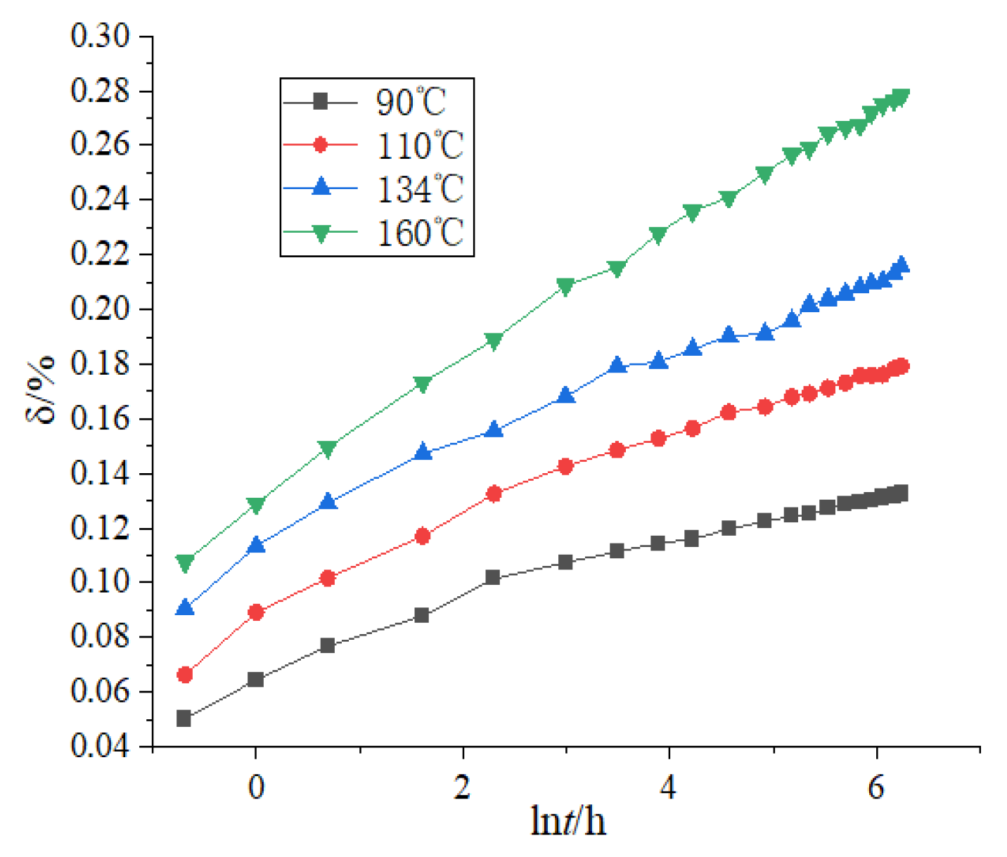
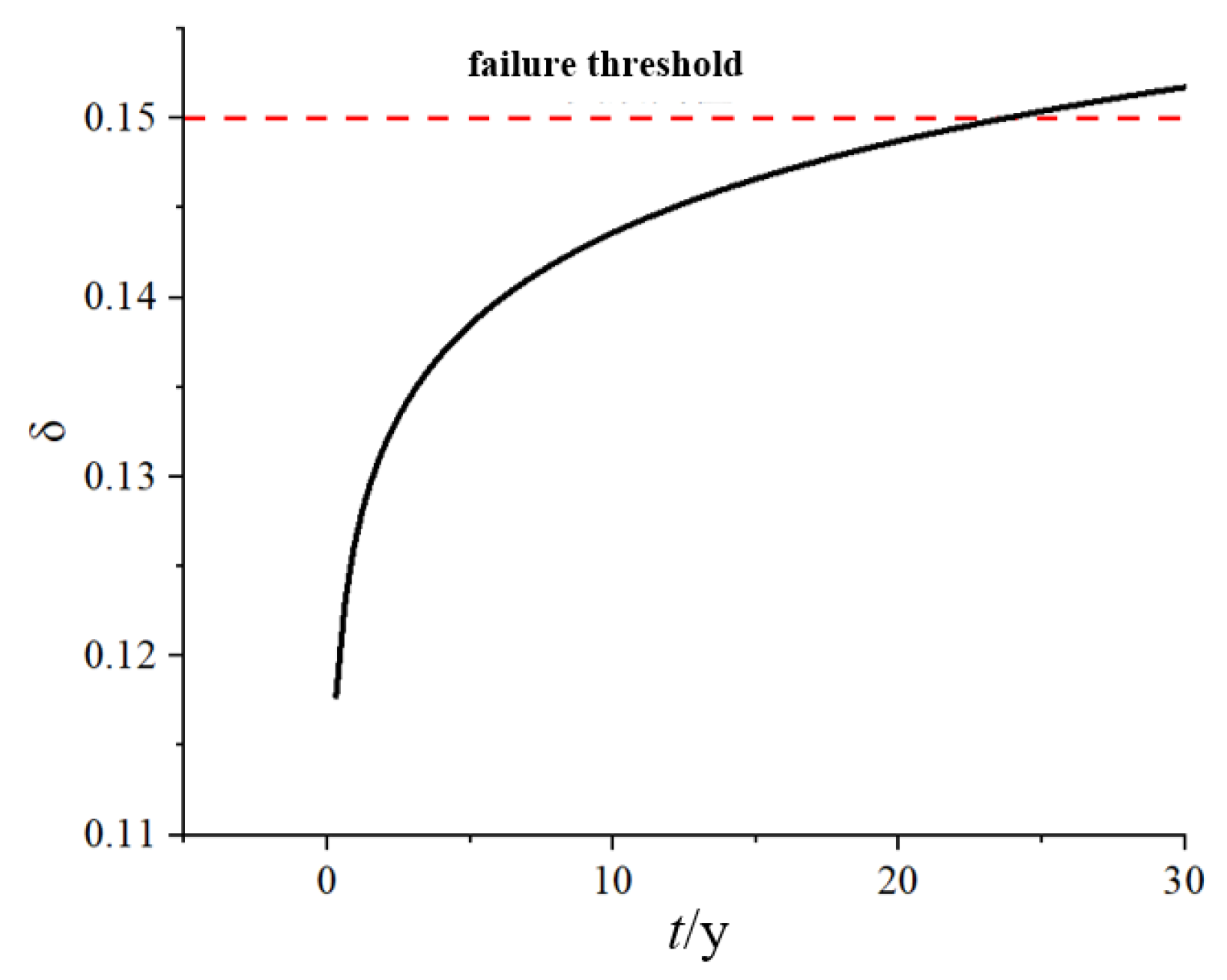
This paper examines the primary causes of electromagnetic release degradation, identifies the rate of loss of the spring reaction force and the striker counterforce as the characteristic quantity of degradation, chooses temperature as the accelerating stress to perform an accelerated life test on the electromagnetic release inside the low-voltage DC circuit breaker, obtains the degradation curves of the electromagnetic release reaction force under various accelerating temperatures, and deduces them using the Arrhenius equation. It then combines these curves with its failure conditions to obtain the full-life data of electromagnetic release under normal operation and offers theoretical information for estimating the electromagnetic release’s remaining useful life.

(2)

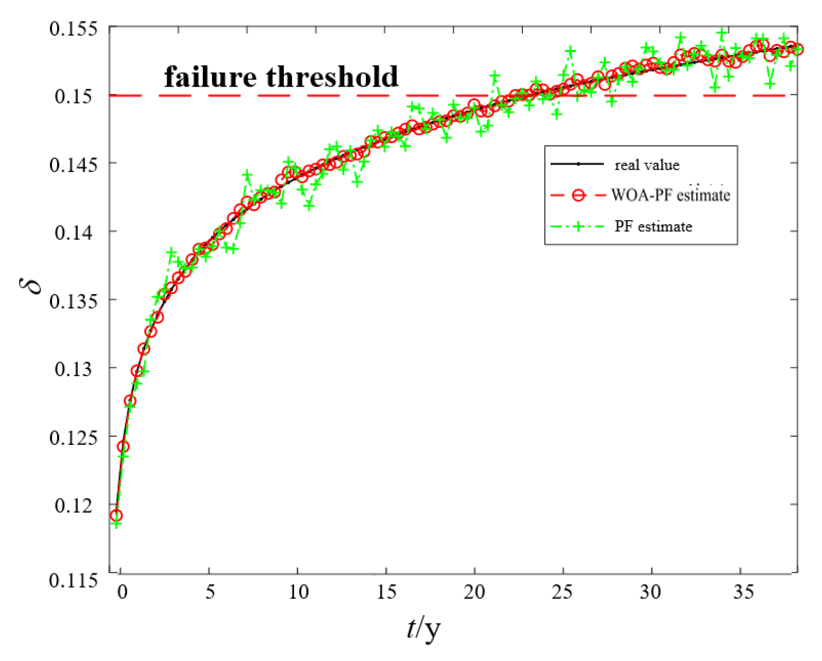
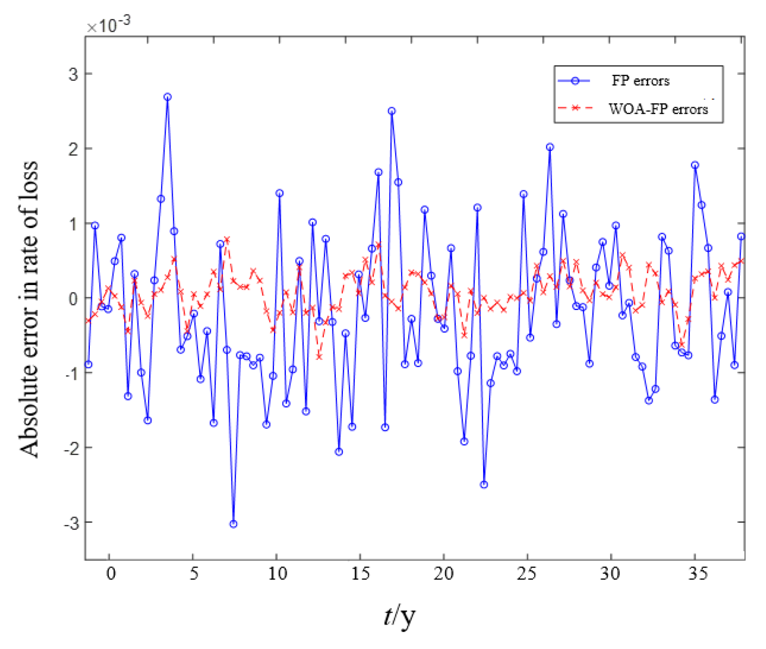
For the problem of particle degradation of traditional particle filter, an improved method of remaining useful life prediction based on whale optimization algorithm is proposed to replace the traditional particle filter resampling process with whale optimization algorithm, so that the particle weights in the particle set are more reasonably allocated. The WOA-PF algorithm and the PF algorithm are used to predict the remaining useful life of an electromagnetic release, and the experimental results show that the WOA-PF algorithm has a higher prediction accuracy than the traditional PF algorithm, and the error accuracy is improved by 2.65%, making it more practical and reliable in predicting the remaining useful life of an electromagnetic release.

References

1. Yan, Y.; Sun, Y.; Guo, W.; Hou, K. Modular Multilevel Solid State Transformer with DC Short Circuit Fault Blocking Capability with Arm Integrated Submodule. Power Syst. Technol. 2023, 43, 1–15. [Google Scholar]
2. Wei, S.; Yu, C.; Chao, S.; Wang, W.; Xie, Y.; Fang, T. Multi-port Commutation-based Hybrid DC Circuit Breaker with Low Conduction Loss Considering Bus Fault. Autom. Electr. Power Syst. 2022, 46, 140–149. [Google Scholar] [CrossRef]
3. Wang, Z.; Gao, Z.; Zhang, J. Protection for Active Distribution Network Considering Short-circuit and Broken-line Faults. Autom. Electr. Power Syst. 2021, 45, 133–141. [Google Scholar] [CrossRef]
4. Dong, B.; Tao, L.; Li, Z.; Zhang, R.; Xu, X.; Wen, T. A Gas Gap Switch Scheme for Commutation Branch of DC Circuit Breakers and Its Induced Breakdown Characteristics. High Volt. Eng. 2022, 48, 4863–4872. [Google Scholar] [CrossRef]
5. Li, B.; Li, P.; Wen, W.; Liu, H. Performance Analysis and Resonant Commutation Method of Mechanical DC Circuit Breaker. Trans. China Electrotech. Soc. 2022, 37, 2139–2149. [Google Scholar] [CrossRef]
6. Zhao, C.; Li, K.; Hu, B.; Ma, D.; Zhao, W.; Zhang, G. Residual Electrical Life Prediction of Low-voltage Circuit Breakers Under Varied Stress. Proc. CSEE 2022, 42, 8004–8016. [Google Scholar] [CrossRef]
7. Sun, S.; Tang, Y.; Wang, J.; Wen, Z.; Gao, H. Life Prediction of Operating Mechanism for Circuit Breaker Based on Multiple Signal Feature Fusion. High Volt. Eng. 2022, 48, 4455–4468. [Google Scholar] [CrossRef]
8. Liu, G.; Li, X.; Wang, Z.; Yue, C. Remaining Life Prediction of Electronic Residual Current Circuit Breaker Based on Wiener Process. Trans. China Electrotech. Soc. 2022, 37, 528–536. [Google Scholar] [CrossRef]
9. Liu, H.; Lin, Y.; Chen, Y.; Zhou, E.; Peng, B. A study on resampling strategy of intelligent particle filter based on genetic algorithm. J. Electron. Inf. Technol. 2021, 43, 3459–3466. [Google Scholar] [CrossRef]
10. Tian, M.; Bo, Y.; Chen, Z.; Wu, P.; Zhao, G. Firefly algorithm intelligence optimized particle filter. Acta Autom. Sin. 2016, 42, 89. [Google Scholar] [CrossRef]
11. Xie, Y.; Wang, S.; Fernandez, C.; Yu, C.; Fan, Y.; Cao, W.; Chen, X. Improved gray wolf particle filtering and high-fidelity second-order autoregressive equivalent modeling for intelligent state of charge prediction of lithium-ion batteries. Int. J. Energy Res. 2021, 45, 19203–19214. [Google Scholar] [CrossRef]
12. Han, X.; Wu, B.; Wang, D. Firefly Algorithm with Disturbance-Factor-Based Particle Filter for Seismic Random Noise Attenuation. IEEE Geosci. Remote. Sens. Lett. 2020, 17, 1268–1272. [Google Scholar] [CrossRef]
13. Gong, Z.; Gao, G.; Wang, M. An Adaptive Particle Filter for Target Tracking Based on Double Space-Resampling. IEEE Access 2021, 9, 91053–91061. [Google Scholar] [CrossRef]
14. Zhu, F.; Fu, J.-Q. A Novel State-of-Health Estimation for Lithium-Ion Battery via Unscented Kalman Filter and Improved Unscented Particle Filter. IEEE Sens. J. 2021, 21, 25449–25456. [Google Scholar] [CrossRef]
15. Feng, W.; Deng, B. Global convergence analysis and research on parameter selection of whale optimization algorithm. Control. Theory Appl. 2021, 38, 641–651. [Google Scholar] [CrossRef]
16. Liang, Z.; Han, Q.; Zhang, T.; Tang, Y.; Jiang, J.; Cheng, Z. Nonlinearity Compensation of Magneto-Optic Fiber Current Sensors Based on WOA-BP Neural Network. IEEE Sensors J. 2022, 22, 19378–19383. [Google Scholar] [CrossRef]
17. Tsakonas, E.E.; Sidiropoulos, N.D.; Swami, A. Optimal Particle Filters for Tracking a Time-Varying Harmonic or Chirp Signal. IEEE Trans. Signal Process. 2008, 56, 4598–4610. [Google Scholar] [CrossRef]
18. Yu, Z.; Wang, Y.; Yang, P.; Zhao, T. RUL prediction of cable retracting vehicle battery based on improved particle filter. Coal Sci. Technol. 2022, 50, 289–296. [Google Scholar] [CrossRef]
19. GB/T 14048.2—2020; Low-Voltage Switchgear and Controlgear—Part 2: Circuit-Breakers. State Administration of Market Supervision and Administration of the People’s Republic of China, Standardization Administration of the People’s Republic of China. Standards Press of China: Beijing, China, 2020. (In Chinese)
Figure 1. Flowchart of the WOA-PF algorithm.
Energies 17 00670 g001
Figure 2. Constant temperature test chamber.
Energies 17 00670 g002
Figure 3. Force measuring device.
Energies 17 00670 g003
Figure 4. Reaction curve with time.
Energies 17 00670 g004
Figure 5. Reaction loss rate and logarithmic curve of time.
Energies 17 00670 g005
Figure 6. Degradation curve of reaction performance of electromagnetic release device.
Energies 17 00670 g006
Figure 7. Comparison of prediction results of WOA-PF and PF.
Energies 17 00670 g007
Figure 8. Comparison of prediction error between WOA-PF and PF.
Energies 17 00670 g008