Effect of the Degree of Hybridization and Energy Management Strategy on the Performance of a Fuel Cell/Battery Vehicle in Real-World Driving Cycles

Abstract

The study utilizes open-access data to generate power demand curves for a hybrid automotive system, testing twelve configurations with three different energy management strategies and four values for the degree of hybridization (DOH), the latter representing the share of the total power of the vehicle powertrain supplied by the battery. The first control logic (Battery Main—BTM) uses mainly batteries to satisfy the power demand and fuel cells as backup, while in the other two controllers, fuel cells operate continuously (Fuel Cell Main—FCM) or within a fixed range (Fuel Cell Fixed—FCF) using batteries as backup. The results are assessed in terms of H₂ consumption, overall system efficiency, and fuel cell predicted lifespan. The battery is heavily stressed in the BTM and FCF logics, while the FCM logic uses the battery only occasionally to cover load peaks. This is reflected in the battery’s State of Charge (SOC), indicating different battery stress levels between the BTM and FCF modes. The FCF logic has higher stress levels due to load demand, reducing battery lifetime. In the BTM and FCM modes, the fuel cell operates with variable power, while in the FCF mode, the fuel cell operates in a range between 90 and 105% of its rated power to ensure its lifetime. In the BTM and FCM modes, hydrogen consumption decreases at almost the same rate as the DOH increases, due to a decrease in battery capacity and a smaller amount of hydrogen being used to recharge it. In contrast, the FCF control logic results in a larger fuel consumption when the DOH decreases. In terms of FC durability, the FCF control logic performs better, with a predicted lifetime ranging from 1815 h for DOH = 0.5 to 2428 h for DOH = 0.1. The FCM logic has the worst performance, with a predicted lifetime of 800 to 808 h, being almost insensitive to the DOH variation. Simulations were performed on two different driving cycles, and similar trends were observed. Simulations taking into account fuel cell (FC) performance degradation showed an increase in hydrogen consumption of approximately 38% after 12 years. Overall, this study highlights the importance of optimizing control systems to improve the performance of fuel cell hybrid vehicles, also taking into account the component of performance degradation.

1. Introduction

The increasing concern about the environmental impacts of fossil fuels and the need to reduce greenhouse gas emissions has led to a continuous increase in the penetration of renewable energy sources [1]. Renewables grew by 4% in 2018 (and electricity production by 7%) under the combined effects of government support, technological advancement, and emission limits, accounting for nearly 25% of the growth in global energy demand [2]. The fastest-growing electricity production sources are solar photovoltaics (PV) and wind power (270 TWh and 400 TWh in 2022) [3]. The primary disadvantage of renewable energy sources is their intermittent nature [4]. When renewable energy sources are unavailable, auxiliary power units must be used to match the demand. Innovative storage solutions, such as hydrogen or batteries, can be effectively utilized to store, and subsequently convert, excess renewable energy [5]. The IEA also stressed the importance of scaling up hydrogen-based technologies and adopting them in sectors where its diffusion is still scarce such as transport, buildings, and power generation. In fact, electric vehicles (EVs) offer a zero-emission alternative to conventional combustion engines and have the potential to revolutionize the transportation sector [6]. Different alternative solutions have been raised in recent years, but one effective approach to improving the performance and efficiency of EVs consists of the integration of fuel cells (FC) with batteries, constituting Hybrid EVs (HEV). However, this integration presents several challenges, such as managing the power distribution, ensuring the durability and reliability of the fuel cell stack, and addressing the high costs associated with these components [7]. The energy management system (EMS) is responsible for coordinating the power distribution between the fuel cells and batteries feeding the electric motor. Several types of EMSs have been proposed in the literature, which can be broadly classified into deterministic rule-based and optimization-based control strategies [8]. Rule-based strategies rely on predefined rules and thresholds which are set based on the designer’s experience and knowledge. Most of the rule-based EMSs adopt fuzzy logic controllers [9,10]. The optimization-based strategies, on the other hand, seek to minimize or maximize specific performance criteria, such as fuel consumption or emissions, through mathematical optimization techniques. However, these methods can be computationally intensive and may require accurate modeling of the system components [11,12]. Moreover, the evolution of HEVs to autonomous vehicles underlines the importance and huge impact on the development of EMSs. In fact, one major challenge in the field of vehicle control is maintaining the yaw stability and path-tracking accuracy of electric vehicles under varying driving conditions. Wu et al. [13] suggested a coordinated control strategy that allowed for enhancement of the yaw moment control (DYC) and a path-tracking control, while Meng et al. [14] developed an integrated an object detection/tracking system, exploring the surrounding environment and providing the ego vehicle with information about the object’s identity (ID), speed, and orientation. This information is then used to facilitate other modules, such as prediction, planning, and control.

Several studies investigated the performance of HEVs. Most of them were conducted using standard driving cycles, such as the New European Driving Cycle (NEDC) or the Federal Test Procedure (FTP). ARTEMIS driving cycles were used by Marx et al. [15] to reproduce three different scenarios: urban, rural, and highway. They modeled a hybrid fuel cell/battery system including a single energy management strategy. Simulations considered various hybridization rates of the system, i.e., the ratio between battery-provided power and the total power. High hybridization rates perform better in terms of fuel efficiency and system durability, whereas low hybridization rates lead to a lower battery depth of discharge. Alpaslan et al. [16] used ECE-15 and JPN 10-15 drive cycles to simulate the performance of a HEV. The work highlighted the beneficial effect of installing hydrogen systems and supercapacitors on powertrain technologies despite the presence of some issues such as the volume of hydrogen system and system duration. Ma et al. [17] developed a multi-objective energy management strategy for a fuel cell hybrid electric vehicle that considers how power is distributed between the lithium-ion battery and the PEM fuel cell. The optimized EMS prevented fuel cell degradation, caused principally by frequent start–stop cycles and rapid load changes, while still keeping the battery state of charge at a desired level, with a reduced fuel consumption of 7%. However, these standardized cycles do not accurately represent real-world driving conditions, leading to discrepancies between simulated and actual vehicle performance [18]. Datasets such as the Vehicle Energy Dataset (VED) [19], or the Assessment and Reliability of Transport Emission Models and Inventory Systems (ARTEMIS) [20], provide valuable insights into the actual energy consumption and emissions of vehicles under realistic driving conditions were assessed. Sagaria et al. [21] compared the real-world driving scenarios of a passenger battery and a fuel cell electric vehicle (BEV, FCEV), with a conventionally powered one. They obtained encouraging results, with the BEV and FCEV energy consumptions equal to 23% and 65% of the internal combustion engine, respectively. In terms of energy source combinations, it was calculated that combining a battery and fuel cell can increase the vehicle’s range by 10%. On the other hand, combining a battery and an ultra-capacitor can extend the battery life by 10% with minimal impact on the range. In addition to the usual power management approach that considers hydrogen consumption, Wang et al. [22] developed a system that also accounts for the device’s degradation. For their simulations, a campus drive cycle at the University of Delaware was considered representative of a typical urban transit loop. The results showed that, by considering degradation models, the fuel cell’s lifespan could be successfully increased at the expense of a faster rate of battery capacity decay, which lowers the vehicle’s average operating cost during its lifetime. The same trend was observed by Hahn et al. [23] (even if for simulated driving cycles), emphasizing that appropriate system operating parameters can partially mitigate the decline in efficiency caused by degradation. Moreover, increasing the stack lifetime could lead to decreased efficiency. Recent studies were focused on discerning micro-health parameters, which represent the operational condition of both the active material and the electrolyte within the battery. Alterations in these micro-health parameters serve as indicators for assessing the internal health status of the battery [24]. There is a lack of literature regarding the optimization of energy strategies for hydrogen-based vehicles running real driving cycles that consider the lifetime too.

The novelty of this paper is the investigation of the influence of the DOH and EMS on the performance and the lifetime of an HEV; moreover, this study analysed different real-world driving cycles using the ARTEMIS and VED databases. To this purpose, an HEV and the EMS were modelled in the framework of TRNSys 18 software [25]. According to the energy demand of the driving cycles, the technologies employed were properly sized. Simulations were carried out using three different EMSs and four different DOHs. The results were used to compare the EMSs in terms of hydrogen consumption, efficiency, battery cycles, and predicted life of the fuel cell. The presented considerations can serve as a starting point for developing multi-objective optimization and smarter EMSs, taking into account the system efficiency, component lifespan, and economic parameters for FCEVs.

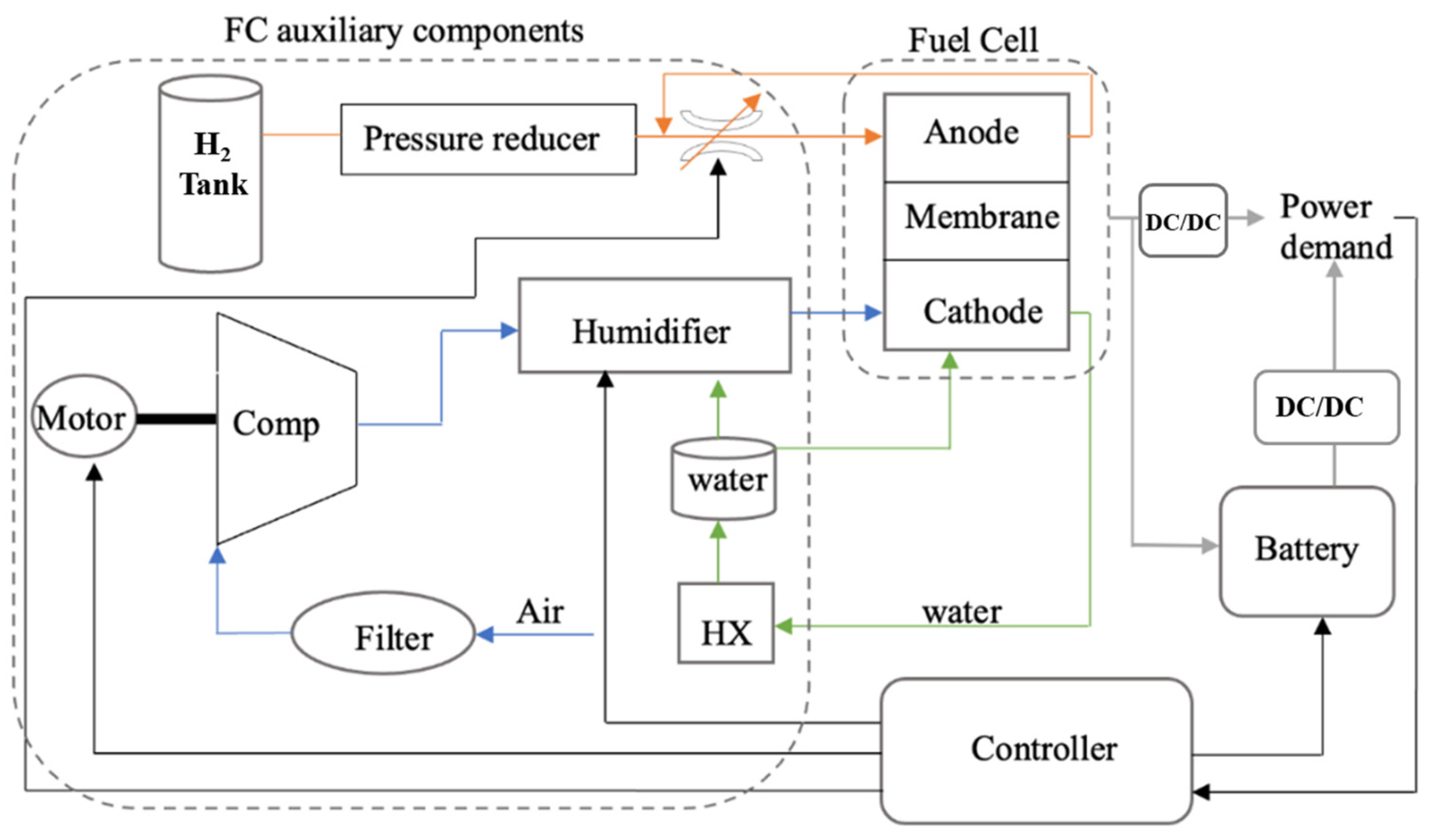
2. Methodology and Adopted Models

The simulated system was composed of all the HEV powertrain components, including an FC stack, a parallel-connected battery pack, and auxiliary equipment (such as a compressor, humidifier, hydrogen tank, and water management system). A unidirectional boost DC/DC converter was used to connect the PEMFC to the system, ensuring stable operation despite load variations, and protecting it from high frequency and surge load power demand to extend its lifetime. The DC/DC converter also acted as the EMS actuator, providing the FC output power. The batteries were connected with a bidirectional converter, regulating output voltage and current with an assumed efficiency of 93%. The EMS controlled the air and hydrogen compressors to avoid fuel starvation and recirculates unreacted hydrogen to the fuel cell inlet. The humidifier regulated the FC cathode humidity (at the anode, the inlet hydrogen has 100% of relative humidity), and the FC operating temperature was controlled through the heat exchanger and water pump by the EMS to maintain an exit relative humidity of 85–95% and prevent membrane drying. The EMS acted as the central control unit, coordinating the actions of all components. A schematic representation of the entire system is shown in Figure 1. The power demand of the vehicle includes the energy required to meet the needs of auxiliary power (such as compressors, humidifiers, and pumps) and traction power. At each time step, the EMS determines the power requested by the vehicle to perform the selected drive cycle and satisfies it through a combination of fuel cells and batteries output. To control the FC power, the EMS adjusts the amount of air and hydrogen supplied to the fuel cell and regulates the step ramp of FC power while providing the missing power from the batteries until the load is satisfied.

2.1. Energy Management System (EMS)

Three distinct control strategies were developed in the design methodology to investigate the system behavior. These strategies were based on the constraints described in [26,27]. The electric power required by the system can be supplied by a combination of FC and battery or by either one of them alone. Hybrid systems were proposed in [28,29] to address the slow response of fuel cells. The EMS of a hybrid system plays a critical role in ensuring the proper functioning of the entire system. The operation of the battery system is limited to mitigate degradation. To ensure its health and longevity, its charging power is programmed on the basis of the current state of charge (SOC). The SOC of the battery is physically constrained between 0% and 100%, but it must fall within a narrower range limited by the designated lower ($SO{C}_{min}$) and upper ($SO{C}_{max}$) limits to prevent excessive depletion and overcharging. For this reason, in all the simulated cases, $SO{C}_{min}$ was assumed equal to 40% and $SO{C}_{max}$ equal to 80%.

To control the charging and discharging rates, the battery voltage and/or current are commonly restricted, which results in power ($P_b$) upper and lower limits:

$$P_{b,min}\le P_b\le P_{b,max}$$

(1)

On the other side, the FC must maintain an idling operation of about 10% of its nominal power (P_fc) to prevent shutdown cycles. Thus, its power must remain within a range that does not fall outside its lower limit (P_fc,min) and upper limit (P_fc,max) [30].

The main difference between the control systems considered in this study is how the FC and batteries provide power to meet the load. Three different cases were evaluated:

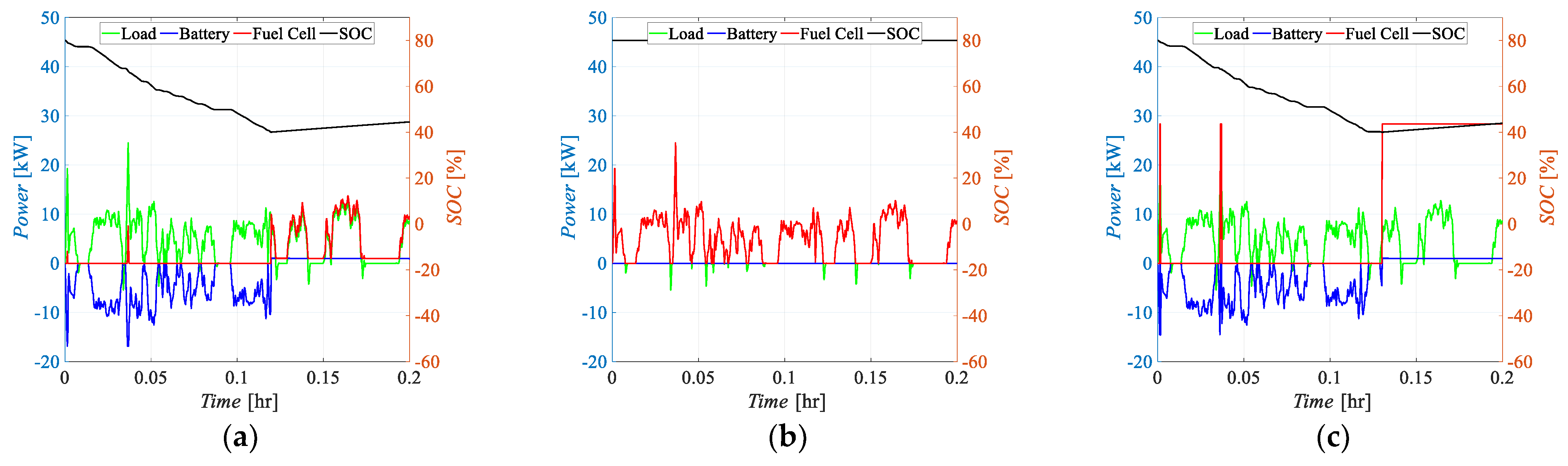
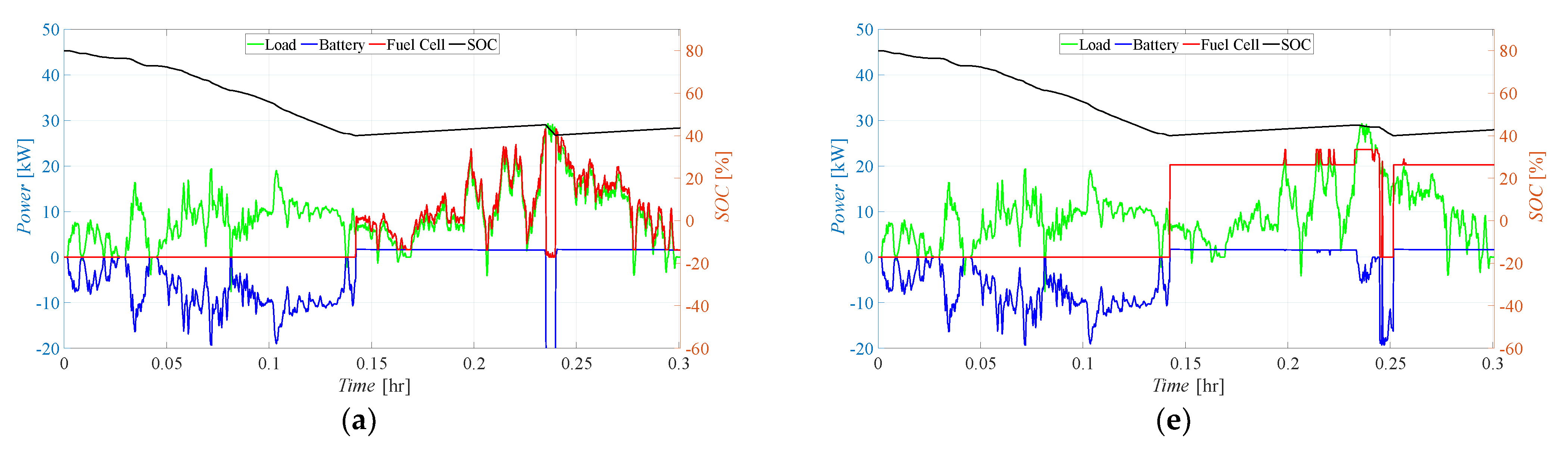
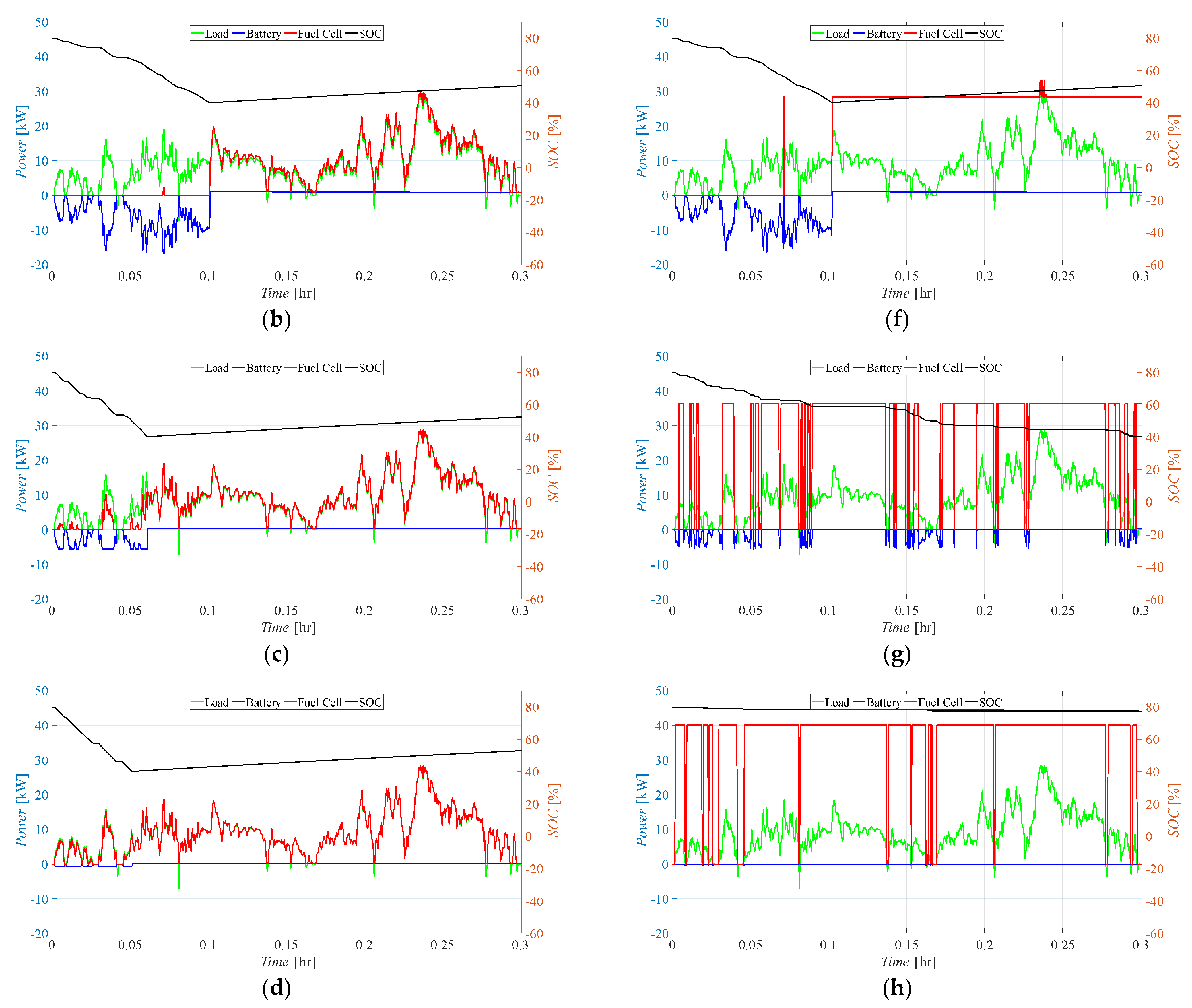
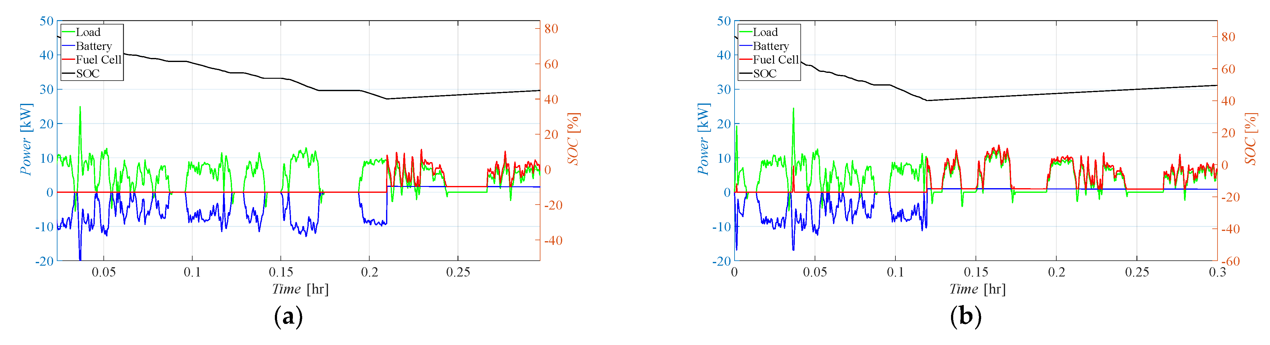
• Battery Main (BTM): In this case, the power is provided mainly by the batteries, with the FC activating only to cover the peaks or to recharge the batteries when their state of charge falls below $SO{C}_{min}$ (in this case also covering the load);
• Fuel Cell Main (FCM): In the second control logic, the FC operates continuously in response to the load, with additional support from batteries during demand peaks. The batteries are charged when the load is smaller than the FC maximum power and SOC is smaller than $SO{C}_{min}$;
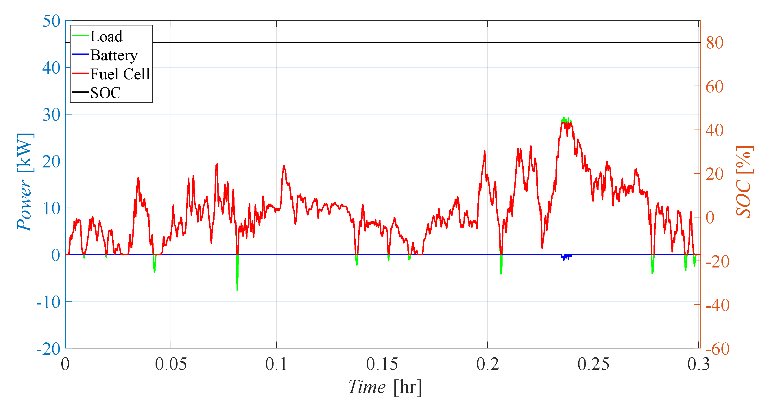
• Fuel Cell Fixed (FCF): In the third scenario, the FC operates only in the range between 90 and 105% of its nominal power (P_fc,nom = 0.8·P_fc,max) to protect its lifespan. The batteries cover the peaks and follow the load when it is smaller than the FC operating range. In the case that the batteries’ SOC becomes smaller than $SO{C}_{min}$, and the load is smaller than the FC’s working power range, the FC covers the load and recharges the batteries. Since the FC always works between 90 and 105% of its nominal power, during battery recharge it may result in fuel waste when the load is very small. If the load is larger than 1.05·P_fc,nom, batteries should cover the gap, even if the SOC is smaller than $SO{C}_{min}$, until needed or until they can.

2.2. Fuel Cell Degradation Prediction

In automotive operations, an FC stack is expected to run under a wide range of operating conditions, including variable humidity and temperature [31], and this strongly affects its performance. The PEMFC performance variations are due to working conditions such as water operation, poor temperature operation, gas starvation, impurities, and load cycling [32]. The load cycling can lead to platinum agglomeration on the catalyst layer, lowering the active surface area. This phenomenon is predominant at the catalyst layer on the cathode side because the platinum particles could only be dissolved on higher potentials. The potential on the interface of the membrane and cathode is much higher than the potential on the anode side. Therefore, the cathode catalyst layer is much more vulnerable than the layer on the anode side to the load cycling. The potential cycling could also lead to carbon corrosion and membrane degradation on the catalyst layer or the gas diffusion layer [33]. Based on operating mode investigations, many researchers inspected the effect of operating conditions on the fuel cell stack’s durability [34,35]. Zhao et al. [36] analyzed the decay characteristics of a fuel cell stack based on an actual road test condition for a bus in China. They fitted experimental data to obtain a semiempirical formula to predict the lifetime of the device. The authors claimed that, using the device to satisfy an intermittent and variable load, the fuel cell duration was almost 5000 h, while it can reach 30,000 h in the case of continuous operations at a fixed point. Fuel cell degradation is deeply influenced by vehicle operating conditions, i.e., start–stop conditions, idling, load changing, and high-power load. In [37], the degradation related to each of them was investigated and modeled, and such a model was taken as a reference in the present work. For the sake of clarity, a brief description of the main aspects of the degradation model are reported here. Further details can be found in the cited work. For evaluating FC degradation, each driving cycle can be described as a sum of four different operating behaviors:

$$\mathrm{Driving} \mathrm{Cycle}=f\left\{n_1, t_1, n_2, t_2\right\}$$

where f indicates a generic function,$n_1$ is the average start–stop cycles per hour, $t_1$ represents the average idling time per hour, $n_2$ represents the average cycles during the load change phase, and $t_2$ is the average time in hours of the high-power load operation. In [38], the authors performed tests to quantify the voltage degradation of each of the phases of a driving cycle, finding the values reported in

Table 1. PEM fuel cell voltage degradation rate [37].

Operating Conditions	Voltage Degradation Rate
Start–Stop	$V_1=13.79 \mathsf{\mu }\mathrm{V}/\mathrm{cycle}$
Idling	$U_1=8.662 \mathsf{\mu }\mathrm{V}/\mathrm{h}$
Load Change	$V_{2 }=0.4184 \mathsf{\mu }\mathrm{V}/\mathrm{cycle}$
High Power Load	$U_{2 }=10.00 \mathsf{\mu }\mathrm{V}/\mathrm{h}$

. The total degradation rate $V_{deg}$ is then computed as a superposition of effects:

$$V_{deg}=n_1{V}_1+t_1{U}_1+n_2{V}_2+t_2{U}_2$$

(2)

Indicating with $\Delta V$ the maximum single fuel cell voltage degradation, the fuel cell life can be computed as

$$T_{FC}=\frac{\Delta V}{k·V_{deg}}$$

(3)

where k = 1.72, a tuning coefficient to align the tests results with the real driving cycle measurements. This semiempirical model was validated in [37] by comparing the prediction with the real degradation of an FC bus.

3. Simulation Details

The performance of an HEV in real driving conditions was evaluated under four possible sizes of the vehicle powertrain (DOHs). For each configuration, the three different control logics described in Section 2.1 were tested, while maintaining the system’s main scheme and characteristics, as shown in Figure 1.

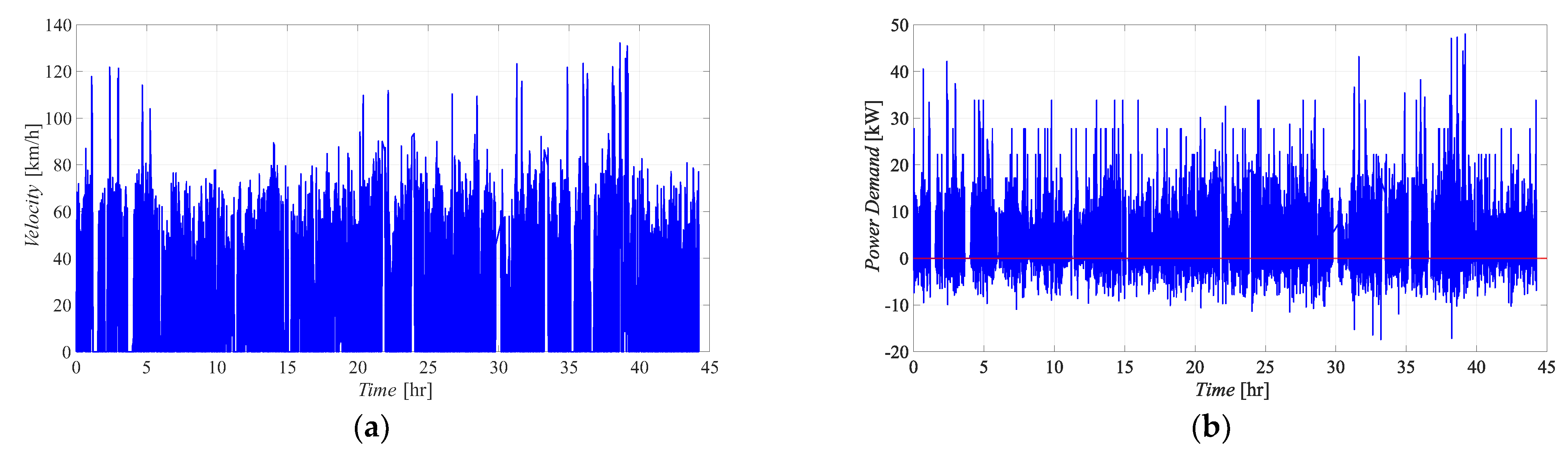
3.1. Case of Study and Generation of Power Demand Curve

Researchers from the University of Michigan (UM), the Argonne National Lab, and the Idaho National Lab recently compiled a comprehensive dataset (VED) of fuel and energy information obtained from 383 privately owned cars in Ann Arbor, MI, USA [14]. This publicly available dataset includes GPS data capturing the vehicles’ trajectories, as well as time series data on fuel consumption, energy usage, speed, and auxiliary power consumption. Among the tracked vehicles, three were fully electric, for which the propulsion system was similar to the one considered here. For this reason, one of these EVs was selected to generate the power demand curve that the novel hybrid system needs to satisfy. Specifically, data from the 2013 Nissan Leaf (vehicle no. 455 of the dataset) were extracted and extrapolated, and all the routes traveled in one year were fused into a single data curve. This extrapolation was performed using a Matlab (v22b) script, scanning the whole dataset and selecting only the trips from the selected vehicle. Given privacy concerns, the dataset underwent filtration to de-identify personally identifiable information. Consequently, certain routes exhibited non-null velocity values at their beginning or conclusion. This discrepancy yielded unphysical vehicle acceleration and deceleration, thereby leading to elevated load demand values. To address this issue, when the initial or final velocity deviated from zero, a consistent acceleration and deceleration were imposed at the beginning and end of each vehicle trip. This assumption involved employing a constant acceleration (a = 2.42 m/s²), determined as 80% of the maximum acceleration of the Toyota Mirai FCEV. Velocity profiles extrapolated from the VED dataset for the selected vehicle are shown in Figure 2a. The routes were mainly urban (the mean velocity is around 34 km/h) but the velocity peaks show that some extra-urban routes have also been traveled, making the dataset appropriate to carry out general considerations.

The second real driving cycles database used was ARTEMIS [20]. The ARTEMIS project was funded by the European Commission as part of the 5th Framework Research Programme, DG TREN. As told before, the driving cycles collected within ARTEMIS are divided into three classes: rural roads, urban, and motorways. In the present work, the rural roads driving cycle was selected, characterized by an average speed of 48 km/h.

It is important to note that while the VED database was used to generate a one-year trip (corresponding to 44.3 driving hours), the selected ARTEMIS driving cycle lasts only 0.3 h.

If the speed profiles are known, the vehicle acceleration can be evaluated and the traction power ($P_{wheel}$) can be calculated by solving the dynamic equation for the longitudinal motion of the vehicle:

$$M\frac{dv}{dt}=F_{tract}+F_{drag}+F_{roll}+F_{grade}.$$

(4)

where M is the vehicle mass, $F_{tract}$ is the traction force that the electric motor should provide to ensure the acceleration $dv/dt$, $F_{drag}$ is the drag resistance of the vehicle, $F_{roll}$ is the rolling resistance of the tires, and $F_{grade}$ is the grading resistance [38]. By inverting Equation (4), it is easy to calculate the traction force, the traction energy required by the vehicle at each time interval, and the traction power $P_{wheel}$. The power demand to be met by the traction system ($P_{wheel}$) is then calculated as:

$$P_{demand}=P_{wheel}/\eta$$

(5)

where $\eta$ is the total efficiency of the system, including the efficiency of the motor and of all the electrical devices between the power units (i.e., the FC and the battery) and the motor. In the present study, 0.8 is taken as the motor efficiency and 0.8 for the rest, giving $\eta =0.64$ as the total efficiency.

As an example, Figure 2b shows the power demand curve for one of the vehicle configurations selected from the VED. The positive peaks represent the effective demand required by the electric motor during acceleration, while negative values indicate vehicle braking. For the sake of clarity, the battery power is represented adopting an opposite sign convention, that is, negative when the battery is discharging, and positive when it is recharging. No regenerative braking system was considered.

3.2. Vehicle Powertrain Sizing

The sizing of the powertrain system was chosen by assuming an electric motor with a power P_mot = 50 kW to cover the peaks of the selected yearly routes of the vehicle as shown in Figure 2b. By assuming an efficiency of the motor drive η_mot = 0.89 [38], the total power that the battery and the fuel cell must guarantee is P_tot = 56 kW. As explained in Section 1, the hybridization of a fuel cell system with a peaking power source emerges as an effective strategy for mitigating the challenges associated with vehicles powered exclusively by fuel cells. In this case, the total power needed by the vehicle was assumed to be covered by an FC stack and a battery pack by using different possible configurations. The degree of hybridization, already defined as the ratio of the battery maximum power (P_b,max) to the total power of the powertrain (P_tot = P_b,max + P_FC,max), influences both the system design and the performance and cost of the system.

$$DOH [\%]=\frac{P_{B,max}}{P_{B,max}+P_{FC,max}}\ast 100$$

(6)

A DOH of 0% indicates that the FC supplies all the power, while 100% indicates that the batteries do it. In this study, four different DOHs have been analyzed, ranging from 0.5 to 0.001. Usually, smaller DOHs are more suitable for light vehicles [15], thus, in the present study, the simulated DOHs do not exceed 0.5. From the definition of DOH, known as the P_tot, the maximum power that the battery pack and the fuel cell stack need to guarantee can be easily calculated. By assuming a C-Rate equal to 10, the total capacity of the Lithium-Ion battery pack is computed, while the nominal voltage is considered equal to 310.8 V, according to the electric motor’s characteristics.

The fuel cell was sized considering the voltage to be supplied to the DC/DC converter, which powers the electric motor, was equal to 300 V. Noting the maximum power to be installed in the vehicle, it is possible to calculate the maximum current to be supplied by the FC. If each individual cell operates at a voltage V_c = 0.7 V, the calculation of the cells in the fuel cell stack is given by N = V/V_c = 300/0.7 = 429. The current to be supplied by the FC is the same for all individual cells connected in the series. If the current is known, it is possible from the FC polarization curve to calculate the cross-sectional area of the individual FC. For this FC at the known voltage of 0.7 V, the current density results equal to i = 400 mA/cm². To produce the needed current, the cross-sectional area can be calculated as $A=\raisebox{1ex}{$I$}\!\left/ \!\raisebox{-1ex}{$i$}\right.$ [39].

The vehicle power demand depends on its kerb weight (W_kerb), which, in turn, depends on the system configuration. By decreasing the DOH, the battery pack will be characterized by lower capacities and weights, while the FC system will show the opposite behavior. The components’ weight was calculated by assuming the same specific weights of the FC stack (0.41 kg/kW) and of the battery pack (11.15 kg/Ah) of the Toyota Mirai vehicle. Based on the DOE Technical Targets for Onboard Hydrogen Storage for Light-Duty Vehicles [40], the hydrogen tank capacity (C_tank) was set equal to 5.6 kg. Using the DOE’s projected gravimetric capacity of 0.055 kg H₂/kg for 2025, the total hydrogen system weight (W_fc,sys) was estimated for the four tested configurations. The total weights and the main components’ characteristics are summarized in

Table 2. Sizing of powertrain vehicle system for the four different DOHs. Weights of each component and total vehicle kerb weight are also reported.

	DOH	Pfc,max [kW]	Pbat,max [kW]	Cbat [Wh]	Wbat [kg]	Wfc [kg]	Wfc,sys [kg]	Wkerb [kg]
Pmot	0.5	28.13	28.13	2812.50	100.9	11.43	103.18	1550
50	0.3	39.38	16.88	1687.50	60.5	16.00	107.75	1514
Ptot	0.1	50.63	5.63	562.50	20.2	20.57	112.32	1478
56	0.01	55.69	0.56	56.25	2.02	22.62	114.38	1462

.

4. Results

In this section, the results of the simulations carried out with different control logics, different DOHs, and different driving cycles are presented and discussed. First, the effect of the control logic is assessed (Section 4.1), then the effect of the DOH and of the driving cycles on the vehicle performance are analyzed (Section 4.2 and Section 4.3, respectively). Based on such results, further computations have been performed to do some considerations about FC lifespan duration and how FC degradation affects the overall system performances (Section 4.4).

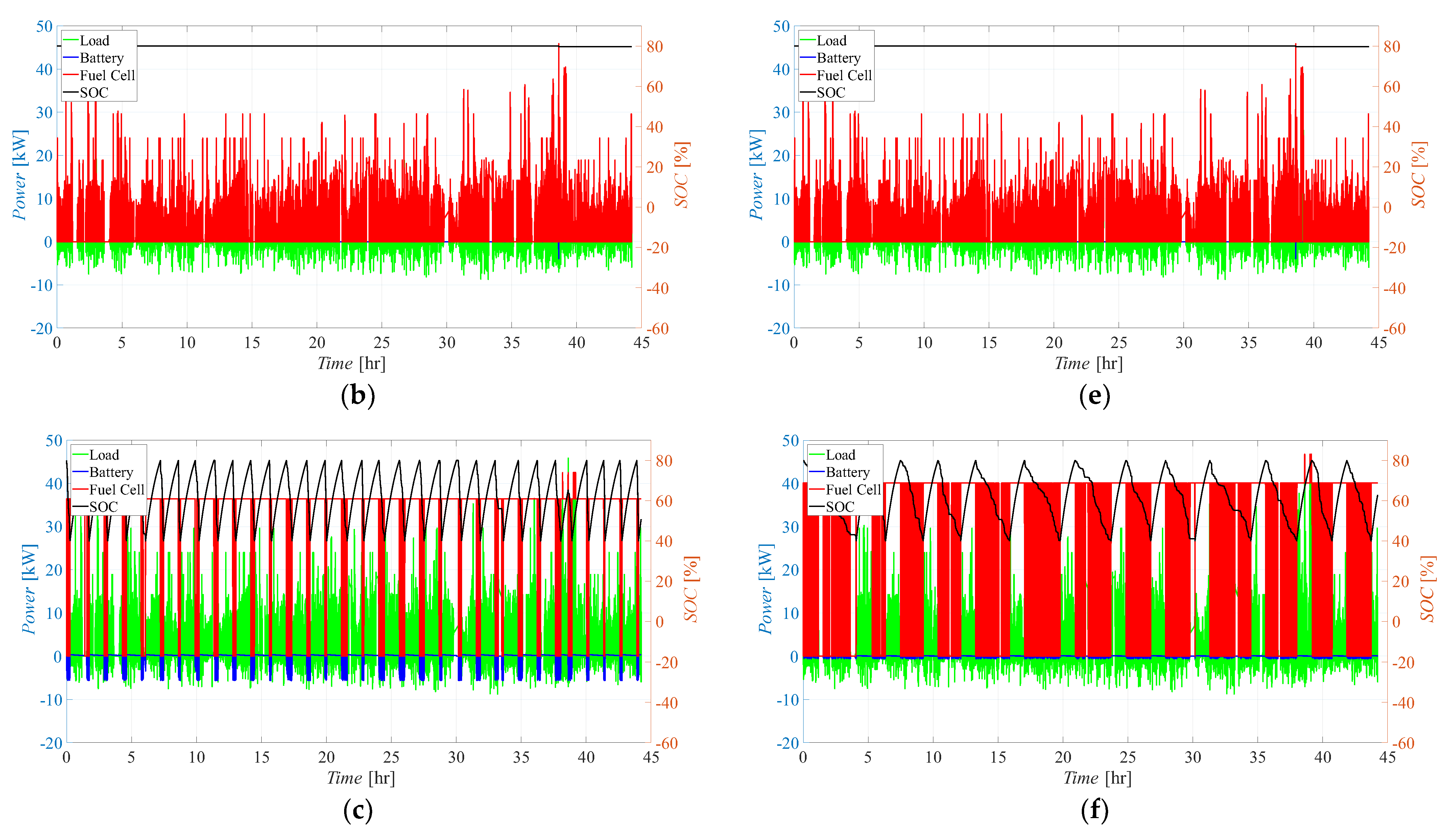
4.1. Effects of the Control Logic

To discuss the effect of the control logic on vehicle performance, in Figure 3, the system behavior is shown considering (for the sake of clarity) only the first 0.2 h of the VED driving cycle. As expected, when the BTM control logic is adopted, the battery is primarily activated, and the FC works only to cover the peaks and when the battery’s SOC goes below its minimum. In the FCM control, the FC responds to the load request. Since in the time interval shown the power demand is below the P_fc,max, the battery is not activated. In Figure 3c, the system behavior under the FCF control logic is represented. In this case, the FC covers the load peaks and/or charges the battery, working always in a fixed range around its nominal power.

Figure 4a–c shows the load, battery, and FC power curves for DOH = 0.5 and the three control logics tested, while in Figure 4d–f, the plots are reported for DOH = 0.3. Figure 5d–f shows the same quantities for DOH = 0.1 and DOH = 0.01, respectively. In the BTM (Figure 4a,d) and FCF (Figure 4c,f) modes, the battery is heavily stressed, with frequent activations and recharges, whereas in the FCM mode (Figure 4b,e), the battery is only used occasionally to cover load peaks. Focusing on SOC behavior, in the BTM mode, the battery is frequently recharged and, in some cases, the load demand does not allow it to be fully recharged (up to SOC_max). In two cases (around t = 38.5 h), the battery’s SOC falls below SOC_min (Figure 4a, blue dashed square). In fact, if the load is greater than the FC maximum power, the battery should cover the gap even if its SOC is below the minimum, otherwise, the vehicle would be forced to stop. A similar behavior can be observed in the FCF simulation: Due to the load demand, the battery recharging is often interrupted, increasing its stress and thus reducing its lifetime. Similarly to what is already noticed in Figure 4a, at t = 38.5 h (Figure 4c, blue dashed square), the SOC drops below its minimum value, and here the SOC approaches 20%, an even lower value than in the BTM case. In the same time interval, the FCM logic performs better: In fact, since the battery is used much less than in BTM and FCF, in the moment the maximum load request is reached, the battery still has enough capacity to overcome the peak, only falling below SOC_min for a few instants and being recharged immediately afterwards.

Regarding the operation of the FC, it should be noted that it operates with variable power in both the BTM and FCM control logics. The only difference is that in the former, the battery covers the base load and the FC (mainly) the peaks, whereas in the latter, the behavior is reversed. In the FCF control logic, the FC operates only in a range between 90 and 105% of its rated power to ensure its lifetime.

These behaviors are reflected in the system’s performance.

Table 3. Hydrogen consumption and fuel cell and system efficiencies for different DOH and control logics.

	Hydrogen Consumption (kg)			FC Efficiency			System Efficiency
DOH	BTM	FCM	FCF	BTM	FCM	FCF	BTM	FCM	FCF
0.50	12.06	11.96	44.88	0.61	0.59	0.5	0.54	0.54	0.15
0.30	11.42	11.33	66.38	0.64	0.61	0.5	0.56	0.56	0.10
0.10	10.88	10.87	86.83	0.67	0.63	0.5	0.58	0.58	0.07
0.01	10.69	10.87	82.13	0.66	0.63	0.5	0.59	0.59	0.08

shows the H₂ consumption and the fuel cell and system efficiencies for the tested DOHs and control logics. The system efficiency considers the energy consumption of both the FC and the battery. The calculation of battery consumption takes into account the SOC difference between the initial and final time intervals. For DOH = 0.5, the FCF logic presents the highest fuel consumption, about four times larger than the BTM and FCM. In fact, the main objective of the FCF logic is to make the FC work under the most stable conditions possible, to reduce its degradation. As already stated, this means that when the power demand is low and the SOC of the battery is below SOC_min, the FC is activated to cover the load and recharge the battery. In this case, the FC operates in the optimal working range but it wastes energy. On the other hand, hydrogen consumption in the BTM and FCM control logics is very similar, with the smallest values predicted in the FCM case. From an efficiency standpoint, it is worth noting that, although the differences in FC efficiency are limited (from 0.61 in the BTM case to 0.5 in the FCF case), the range of system efficiency is wider, from 0.54 in the case of the BTM and FCM modes to 0.15 in the FCF case, making the latter logic very unsuitable for the considered vehicle. The trends are confirmed for all the tested DOHs.

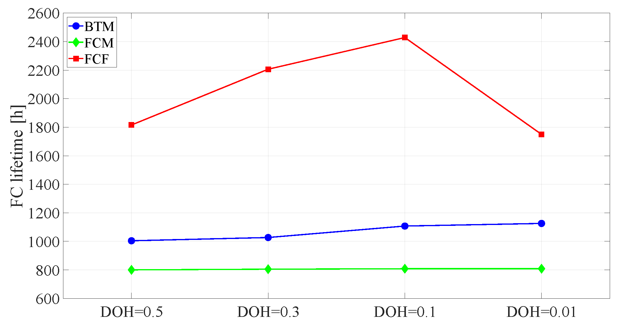
4.2. Effects of the Degree of Hybridization

To assess the influence of the DOH on vehicle performance, some general considerations should be made. The reduction in the DOH leads to a diminution of the weight of the battery pack and the increase in the FC stack weight, eventually resulting in a slight overall reduction in vehicle weight. This, in turn, means a slightly lower load curve. Looking at the BTM control logic, as the DOH decreases (Figure 4a,d and Figure 5a,d), the FC covers the load better, the battery is less stressed and, due to its decreasing capacity, it can be recharged quickly. This results in more frequent (and more complete) recharges, which should increase the battery life.

In the FCM control logic, as the DOH decreases (Figure 4b,e and Figure 5b,e), battery usage also decreases, contributing to the load only in a very narrow time interval at about t = 38.5 h, which corresponds to the highest load request. This could lead to the conclusion that the powertrain is oversized. However, it should be considered that this is only true for this specific drive cycle, which is relatively flat and not very power-demanding.

In the FCF case (Figure 4c,f and Figure 5c,f), the battery is very often recharged due to its lower capacity. For very small DOHs (i.e., 0.01) this trend is the opposite. The reduced battery power is the main cause of this behavior. In fact, the battery is only activated to cover extremely low loads, which is likely to occur at the vehicle’s start. As a result, despite the battery capacity being reduced, the battery intervenes less frequently and less continuously compared to the DOH = 0.1 case. This, in turn, affects the hydrogen consumption and system efficiency, as reported in the following.

The hydrogen consumption (Table 3) shows different behavior as the control logic is changed. In the BTM and FCM cases, the hydrogen consumption decreases (at almost the same rate) as the DOH decreases from 12.06 to 10.69 kg in the BTM case and from 11.96 to 10.87 kg in the FCM. This is because as the DOH is reduced, battery capacity decreases, leading to a progressively smaller amount of hydrogen being utilized for recharging due to its dependence on recharge efficiency.

On the contrary, the FCF control logic results in larger fuel consumption as the DOH decreases (from about 45 to about 82 kg when going from DOH = 0.5 to 0.01, with a peak of about 87 kg for DOH = 0.1). In fact, with this logic, as the DOH is reduced, the FC-rated power rises. Consequently, the quantity of wasted hydrogen increases during periods of low load when the battery requires recharging.

In the case of the smallest simulated DOH, the fuel cell (FC) often activates to cover the large difference with the load due to the small battery power. For the other DOHs, it mostly activates to recharge the battery. This leads to an increase in hydrogen consumption with DOH reduction, but after a peak, the consumption tends to decrease. As a result, the FC efficiency improves as the DOH decreases with the BTM and FCM logics and remains relatively constant in the FCF one. The efficiency of the system remains constant for both BTM and FCM, with the larger efficiency of the BTM being compensated for by smaller hydrogen consumption. The efficiency increases as the DOH decreases. However, in the FCF control logic, the significant increase in hydrogen consumption results in an unacceptable drop in system efficiency, from 15% at DOH = 0.5 to 8% at DOH = 0.01.

4.3. Effect of the Driving Cycles

The impact of various driving cycles on system performance is evaluated using the three control logics and the four DOHs, and is conducted using the selected ARTEMIS driving cycle.

Figure 6 reports the powers (load, battery, and FC) and SOC of the battery curves for FCM control logic. As the curves remain practically identical as the DOH varies, only the case where DOH = 0.5 is reported in the figure. As shown, at approximately 0.24 h, the battery (blue line) is activated to cover the small gap between the load (green line) and the FC power (red line). With a smaller DOH, the battery does not activate at all because the FC can always cover the load. Accordingly, the SOC of the battery (black line) does not change. These findings are in line with those predicted in the case of the VED driving cycle for all the DOHs simulated (Figure 4b,e and Figure 5b,e). In fact, even in the VED simulation, the battery activation reduces as the DOH increases. This means that, at least for the very short time of the ARTEMIS driving cycle, the FCM logic is weakly influenced by the driving cycle.

Even the BTM control logic shows a very small sensitivity to the driving cycle. When working with the ARTEMIS driving cycle (Figure 7a–c), the battery activates first, covering the load, which is quite small. As the SOC decreases down to its lower limit, the FC is activated, covering the load and recharging the battery. As the DOH decreases, the activation of the FC is anticipated, because the battery’s maximum power and capacity decreases accordingly. Therefore, for the smaller DOHs (Figure 7c,d), the FC is activated almost from the start of the driving cycle, covering the load peaks and/or recharging the battery. A similar trend is found with the VED driving cycle, as can be seen in Figure 8, where only the first 0.3 h of the whole driving cycle are reported.

In the FCF control logic, there is a general trend that is the same in both the VED and ARTEMIS driving cycles. In fact, with the ARTEMIS cycle (Figure 7e–h), it is confirmed that the battery is used less as the DOH decreases. These trends agree with the findings in [15], where the control logic adopted aims at optimizing the FC’s life (as in FCF).

The above considerations lead to the general finding that the effect of the driving cycle on the behavior of the control logics is very weak, as confirmed also with a comparison of the trends of hydrogen consumption and the FC and system efficiencies predicted with the VED and ARTEMIS driving cycles. The direct comparison of Table 3 (VED) and

Table 4. Hydrogen consumption and fuel cell and system efficiencies for different DOH and control logics for ARTEMIS driving cycles.

	Hydrogen Consumption (kg)			FC Efficiency			System Efficiency
DOH	BTM	FCM	FCF	BTM	FCM	FCF	BTM	FCM	FCF
0.50	0.105	0.156	0.191	0.557	0.569	0.503	0.605	0.530	0.370
0.30	0.125	0.148	0.344	0.580	0.590	0.504	0.581	0.553	0.227
0.10	0.135	0.141	0.482	0.607	0.605	0.504	0.576	0.568	0.164
0.01	0.139	0.139	0.668	0.620	0.610	0.504	0.575	0.574	0.120

(ARTEMIS) may be misleading because of the different time durations of the cycles. For this reason, in

Table 5. Hydrogen consumption and fuel cell and system efficiencies for different DOH and control logics for the first 0.3 h of the VED driving cycles.

	Hydrogen Consumption (kg)			FC Efficiency			System Efficiency
DOH	BTM	FCM	FCF	BTM	FCM	FCF	BTM	FCM	FCF
0.50	0.025	0.075	0.109	0.610	0.595	0.504	0.748	0.561	0.299
0.30	0.046	0.071	0.295	0.638	0.613	0.504	0.660	0.581	0.132
0.10	0.060	0.068	0.330	0.672	0.628	0.504	0.620	0.595	0.120
0.01	0.066	0.067	0.515	0.656	0.632	0.504	0.604	0.600	0.079

, the hydrogen consumption and the FC and system efficiencies are reported for the first 0.3 h of the VED driving cycle. It is clear that the different driving cycles do not affect the global trends as the DOH varies. Therefore, it is assumed that by repeating the ARTEMIS driving cycle to cover the same time as the VED, the long-term trends (see Section 4.4) remain the same.

4.4. Fuel Cell Lifetime Prediction and Aging Effect on Vehicle Performance

As discussed in Section 2.2, the lifetime of an FC is a function of several parameters, the most important of which are the start–stop cycles, idle time, load change cycles, and high-power load operation time. Here, we have adopted the approach presented in [30] to estimate the lifetime of the FC under the VED load profile (the longer one among the two considered in this study), and consider the FCM control logic.

Since the driving cycle considered is made up of a series of journeys over a period of one year (a total of 44.24 driving hours), the start–stop cycles were calculated by dividing the number of journeys by the total driving time, and it is the same for all the simulations. The average high-power operation time per hour, t₂, was evaluated by summing all the time instants when the FC’s power was greater than or equal to its nominal value and dividing it by the total driving time. The other two quantities were calculated according to their definitions.

Table 6. Load spectrum statistics.

	n1: Start–Stop Cycles (1/h)			t1: Idle Time (min/h)			n2: Load Change Cycles (1/h)			t2: Average High-Power Operation Time (min/h)
DOH	BTM	FCM	FCF	BTM	FCM	FCF	BTM	FCM	FCF	BTM	FCM	FCF
0.50	5.79			8.91	14.67	10.04	379.66	454.05	4.27	0.84	1.01	1.08
0.30				7.66	15.07	7.32	404.53	460.22	4.09	0.16	0.17	0.27
0.10				3.00	15.07	6.09	449.76	460.13	3.05	0.00	0.00	0.02
0.01				2.01	15.07	12.02	458.91	460.13	5.02	0.00	0.00	0.00

summarizes the load spectrum statistics of the considered driving cycle, while Figure 9 shows the predicted lifetime according to Equation (3).

Due to the combination of the changes in the parameters considered, the FC’s life increases with the DOH for all the control logics tested here. The FCF performs better, with a predicted lifetime ranging from 1815 h for DOH = 0.5 to about 2400 h for DOH = 0.1, then decreasing to about 1720 h for DOH = 0.01. When the DOH varies from 0.1 to 0.01 in FCF (Figure 5c,f), since the battery power reduces, its activation time decreases, as well as its usage. On the contrary, the FC is more stressed, so its life is reduced. However, due to the high hydrogen consumption (see Table 3), this control logic is not suitable for the vehicles considered, as written above.

The worst performance in terms of FC life is that of the FCM logic, which ranges from 800 to 808 h, gaining only 1% as the DOH decreases. Again, this was to be expected, as the FC in this case is highly stressed and operates in a very variable manner. The BTM control logic performance is intermediate between the other two. It is worth noting that the prediction is based on the assumption that the vehicle will always repeat the same journey, and then in real cases, the service life could be different.

To study whether FC degradation has any nonlinear effect on FC lifespan and how it affects the system’s performance, simulations were performed for the FCM control logic and DOH = 0.1 in a time interval ranging between 0 to 12 years by changing the FC polarization curve every three years according to Equation (2). The results are reported in Figure 10 in terms of hydrogen consumption and system efficiency. After 12 years, hydrogen consumption for the whole driving cycle increases from 10.87 kg to about 15.0 kg (38%). Accordingly, the system efficiency decreases from 0.58 to 0.42. Figure 10 also shows that, while in the hydrogen consumption (blue line) there is a small nonlinearity, this is fully negligible in the system efficiency. The load spectra produced in the simulations at 9 and 12 years (not shown here for the sake of brevity) remain identical to that of the first year, even when considering the degradation of the FC. Therefore, in this case, the implementation of the FC performance degradation model into the simulation would improve forecast accuracy.

5. Conclusions

This paper presents an analysis of the performance of a hybrid vehicle that uses hydrogen fuel cells and batteries under real-world driving conditions. The simulations explore different control logics and degrees of hybridization, revealing the impact of control logics on battery and fuel cell behavior. The BTM and FCF logics lead to varying levels of stress on the battery due to frequent activations and recharges. In contrast, the FCM logic demonstrates superior performance by using the battery just to cover load peaks. When examining the system’s overall efficiency and hydrogen consumption for different DOHs, the FCM logic stands out with significantly higher efficiency and lower hydrogen consumption compared to the BTM and FCF logics. The FCF logic prioritizes FC stability, which can lead to suboptimal energy utilization during low-demand periods. The BTM and FCM logics demonstrate similar hydrogen consumption and system efficiency. The FCM logic consumes the least amount of hydrogen for larger DOHs, while the two control logics have similar efficiencies for lower DOHs. As the DOH decreases, both the BTM and FCF logics show more frequent and complete battery recharges, which could potentially improve battery life. In the case of the FCM logic, battery results are rarely used for the analyzed driving cycles with low DOHs. Conversely, in the FCF logic, lower DOH results in increased hydrogen consumption and decreased system efficiency, making it unsuitable for the tested vehicle. Simulations were performed on two different driving cycles, and similar trends were observed, demonstrating that the findings can be considered not sensitive to different operating conditions. In the present case, the solution implementing low DOH values and the FCM control logic shows the best results in terms of hydrogen consumption and overall system efficiency even if the FC’s lifespan is not benefited. Simulation results demonstrate that the lifespan of the fuel cell is minimised when FCM logic is employed. In general, the predicted FC lifespan increases with lower DOH values across all control logics but for the FCF. In this case, when the DOH varies from 0.1 to 0.01, the FC is more stressed because of the reduced battery power, resulting in a lower predicted FC lifespan. As expected, the FCF logic exhibits the best performance in terms of predicted lifetime, emphasizing its designed purpose of ensuring regular operating behavior to extend the fuel cell’s longevity. Simulations were also conducted for the FCM control logic and DOH = 0.1, taking into account the fuel cell (FC) performance degradation. The results indicate a 38% increase in hydrogen consumption after 12 years.

Future works should consider longer and more diverse driving cycles to a obtain wider generality of our results. The estimation of the FC’s durability is based on estimations that are not based on real data as, presently, the statistical data are scarce, and almost no consolidated approach to battery pack derating is present in the open literature. Continuous improvement in the model for computing FC and battery derating is expected in the next years and could be applied to the present formulation. Nevertheless, this work represents a credible and up-to-date analysis of alternative configurations for obtaining the most convenient combination of FC and battery use in urban transportation. The considerations presented can be used as a starting point to develop a multi-objective optimization and smarter EMSs considering the system efficiency, component lifespan, and economic parameters for FCEVs.

References

1. Eriksson, E.L.V.; Gray, E.M. Optimization and integration of hybrid renewable energy hydrogen fuel cell energy systems—A critical review. Appl. Energy 2017, 202, 348–364. [Google Scholar] [CrossRef]
2. Lund, P.D.; Lindgren, J.; Mikkola, J.; Salpakari, J. Review of energy system flexibility measures to enable high levels of variable renewable electricity. Renew. Sustain. Energy Rev. 2015, 45, 785–807. [Google Scholar] [CrossRef]
3. IEA. Renewables 2022, Analysis and Forecast to 2027; International Energy Agency: Paris, France, 2023. [Google Scholar]
4. Sun, C.; Negro, E.; Vezzù, K.; Pagot, G.; Cavinato, G.; Nale, A.; Bang, Y.H.; Di Noto, V. Hybrid inorganic-organic proton-conducting membranes based on SPEEK doped with WO3 nanoparticles for application in vanadium redox flow batteries. Electrochim. Acta 2019, 309, 311–325. [Google Scholar] [CrossRef]
5. IEA. The Future of Hydrogen; IEA: Paris, France, 2019; Available online: https://www.iea.org/reports/the-future-of-hydrogen (accessed on 18 January 2024).
6. Manoharan, Y.; Hosseini, S.E.; Butler, B.; Alzhahrani, H.; Senior, B.T.F.; Ashuri, T.; Krohn, J. Hydrogen Fuel Cell Vehicles; Current Status and Future Prospect. Appl. Sci. 2019, 9, 2296. [Google Scholar] [CrossRef]
7. Yue, M.; LambertM, H.; Pahon, E.; Roche, R.; Jemei, S.; Hissel, D. Hydrogen energy systems: A critical review of technologies, applications, trends and challenges. Renew. Sustain. Energy Rev. 2021, 146, 111180. [Google Scholar] [CrossRef]
8. Krithika, V.; Subramani, C. A comprehensive review on choice of hybrid vehicles and power converters, control strategies for hybrid electric vehicles. Int. J. Energy Res. 2018, 42, 1789–1812. [Google Scholar] [CrossRef]
9. García, P.; Torreglosa, J.P.; Fernández, L.M.; Jurado, F. Control strategies for high-power electric vehicles powered by hydrogen fuel cell, battery and supercapacitor. Expert Syst. Appl. 2013, 40, 4791–4804. [Google Scholar] [CrossRef]
10. Niu, L.; Yang, H.; Zhang, Y. Intelligent HEV Fuzzy Logic Control Strategy Based on Identification and Prediction of Drive Cycle and Driving Trend. World J. Eng. Technol. 2015, 3, 215–226. [Google Scholar] [CrossRef]
11. Ettihir, K.H.; Cano, M.H.; Boulon, L.; Agbossou, K. Design of an adaptive EMS for fuel cell vehicles. Int. J. Hydrogen Energy 2017, 42, 1481–1489. [Google Scholar] [CrossRef]
12. Fu, Z.; Zhu, L.; Tao, F.; Si, P.; Sun, L. Optimization based energy management strategy for fuel cell/battery/ultracapacitor hybrid vehicle considering fuel economy and fuel cell lifespan. Int. J. Hydrogen Energy 2020, 45, 8875–8886. [Google Scholar] [CrossRef]
13. Wu, D.; Guan, Y.; Xia, X.; Du, C.; Yan, F.; Li, Y.; Hua, M.; Liu, W. Coordinated control of path tracking and yaw stability for distributed drive electric vehicle based on AMPC and DYC. Proc. Inst. Mech. Eng. Part J. Automob. Eng. 2024. [Google Scholar] [CrossRef]
14. Meng, Z.; Xia, X.; Xu, R.; Liu, W.; Ma, J. HYDRO-3D: Hybrid object detection and tracking for cooperative perception using 3D LiDAR. IEEE Trans. Intell. Veh. 2023, 8, 4069–4080. [Google Scholar] [CrossRef]
15. Marx, N.; Hissel, D.; Gustin, F.; Boulon, L.; Agbossou, K. On the sizing and energy management of an hybrid multistack fuel cell—Battery system for automotive applications. Int. J. Hydrogen Energy 2017, 42, 1518–1526. [Google Scholar] [CrossRef]
16. Alpaslan, E.; Karaoğlanm, U.M.; Colpan, C.O. Investigation of drive cycle simulation performance for electric, hybrid, and fuel cell powertrains of a small-sized vehicle. Int. J. Hydrogen Energy 2017, 48, 39497–39513. [Google Scholar] [CrossRef]
17. Ma, Y.; Li, C.; Wang, S. Multi-objective energy management strategy for fuel cell hybrid electric vehicle based on stochastic model predictive control. ISA Trans. 2022, 131, 178–196. [Google Scholar] [CrossRef]
18. Fontaras, G.; Zacharof, N.G.; Ciuffo, B. Fuel consumption and CO2 emissions from passenger cars in Europe—Laboratory versus real-world emissions. Prog. Energy Combust. Sci. 2017, 60, 97–131. [Google Scholar] [CrossRef]
19. Oh, G.; Leblanc, D.J.; Peng, H. Vehicle Energy Dataset (VED), A Large-Scale Dataset for Vehicle Energy Consumption Research. IEEE Trans. Intell. Transp. Syst. 2022, 23, 3302–3312. [Google Scholar] [CrossRef]
20. Andrè, M. The ARTEMIS European driving cycles for measuring car pollutant emissions. Sci. Total Environ. 2004, 334–335, 73–84. [Google Scholar] [CrossRef] [PubMed]
21. Sagaria, S.; Neto, R.C.; Baptista, P. Assessing the performance of vehicles powered by battery, fuel cell and ultra-capacitor: Application to light-duty vehicles and buses. Energy Convers. Manag. 2021, 229, 113767. [Google Scholar] [CrossRef]
22. Wang, Y.; Moura, S.J.; Advani, S.G.; Prasad, A.K. Power management system for a fuel cell/battery hybrid vehicle incorporating fuel cell and battery degradation. Int. J. Hydrogen Energy 2019, 44, 8479–8492. [Google Scholar] [CrossRef]
23. Hahn, S.; Braun, J.; Kemmer, H.; Reuss, H.C. Optimization of the efficiency and degradation rate of an automotive fuel cell system. Int. J. Hydrogen Energy 2021, 46, 29459–29477. [Google Scholar] [CrossRef]
24. Xu, J.; Sun, C.; Ni, Y.; Lyu, C.; Wu, C.; Zhang, H.; Yang, Q.; Feng, F. Fast Identification of Micro-Health Parameters for Retired Batteries Based on a Simplified P2D Model by Using Padé Approximation. Batteries 2023, 9, 64. [Google Scholar] [CrossRef]
25. TRNSYS 18: A Transient System Simulation Program; Solar Energy Laboratory, University of Wisconsin: Madison, WI, USA, 2017. Available online: https://sel.me.wisc.edu/trnsys (accessed on 18 January 2024).
26. Amin; Bambang, R.T.; Rohman, A.S.; Dronkers, C.J.; Ortega, R.; Sasongko, A. Energy Management of Fuel Cell/Battery/Supercapacitor Hybrid Power Sources Using Model Predictive Control. IEEE Trans. Ind. Inform. 2014, 10, 1992–2002. [Google Scholar] [CrossRef]
27. Ziaeinejad, S.; Sangsefidi, Y.; Mehrizi-Sani, A. Fuel Cell-Based Auxiliary Power Unit: EMS, Sizing, and Current Estimator-Based Controller. IEEE Trans. Veh. Technol. 2016, 65, 4826–4835. [Google Scholar] [CrossRef]
28. Kim, M.; Sohn, Y.S.; Lee, W.L.; Kim, C.S. Fuzzy control based engine sizing optimization for a fuel cell/battery hybrid mini-bus. J. Power Sources 2008, 178, 706–710. [Google Scholar] [CrossRef]
29. Wipke, K.B.; Cuddy, M.R.; Burch, S.D. A user-friendly advanced powertrain simulation using a combined backward/forward approach. IEEE Trans. Veh. Technol. 1999, 48, 1751–1761. [Google Scholar] [CrossRef]
30. Borup, R.; Meyers, R.; Pivovar, B.; Kim, Y.S.; Mukundan, R. Scientific Aspects of Polymer Electrolyte Fuel Cell Durability and Degradation. Chem. Rev. 2007, 107, 3904–3951. [Google Scholar] [CrossRef] [PubMed]
31. Zhao, N.; Chu, Y.; Xie, Z.; Eggen, K.; Girard, F.; Shi, Z. Effects of Fuel Cell Operating Conditions on Proton Exchange Membrane Durability at Open-Circuit Voltage. Fuel Cells 2020, 20, 176–184. [Google Scholar] [CrossRef]
32. Bai, X.; Luo, L.; Huang, B.; Jian, Q.; Cheng, Z. Performance improvement of proton exchange membrane fuel cell stack by dual-path hydrogen supply. Energy 2022, 246, 123297. [Google Scholar] [CrossRef]
33. Nguyen, H.L.; Han, J.; Nguyen, X.L.; Goo, Y.-M.; Le, D.D. Review of the Durability of Polymer Electrolyte Membrane Fuel Cell in Long-Term Operation: Main Influencing Parameters and Testing Protocols. Energies 2021, 14, 4048. [Google Scholar] [CrossRef]
34. Zhao, Y.; Li, X.; Li, W.; Wang, Z.; Wang, S.; Xie, X.; Ramani, V. A high-performance membrane electrode assembly for polymer electrolyte membrane fuel cell with poly(arylene ether sulfone) nanofibers as effective membrane reinforcements. J. Power Sources 2019, 444, 227250. [Google Scholar] [CrossRef]
35. Pivac, I.; Bezmalinović, D.; Barbir, F. Catalyst degradation diagnostics of proton exchange membrane fuel cells using electrochemical impedance spectroscopy. Int. J. Hydrogen Energy 2018, 43, 13512–13520. [Google Scholar] [CrossRef]
36. Zhao, Y.; Wang, Q.; Xu, L.; Hu, Z.; Jia, X.; Qin, Z.; Li, J.; Ouyang, M. Characteristic Analysis of Fuel Cell Decay Based on Actual Vehicle Operating Conditions. In Proceedings of the IEEE 4th International Electrical and Energy Conference (CIEEC), Wuhan, China, 28–30 May 2021. [Google Scholar]
37. Chen, H.; Pei, P.; Song, M. Lifetime prediction and the economic lifetime of Proton Exchange Membrane fuel cells. Appl. Energy 2015, 142, 154–163. [Google Scholar] [CrossRef]
38. Ehsani, M.; Gao, Y.; Longo, S.; Ebrahimi, K. Modern Electric, Hybrid Electric, and Fuel Cell Vehicles, 3rd ed.; CRC Press: Boca Raton, FL, USA, 2018. [Google Scholar]
39. Fragiacomo, P.; Piraino, F.; Genovese, M.; Flaccomio, L.; Dei, N.; Donati, D.; Migliarese Caputi, M.V.; Borello, D. Sizing and Performance Analysis of Hydrogen- and Performance Analysis of Hydrogen- and Battery-Based Powertrains, Integrated into a Passenger Train for a Regional Track, Located in Calabria (Italy). Energies 2022, 15, 6004. [Google Scholar] [CrossRef]
40. DOE Technical Targets for Onboard Hydrogen Storage for Light-Duty Vehicles. Available online: https://www.energy.gov/eere/fuelcells/doe-technical-targets-onboard-hydrogen-storage-light-duty-vehicles (accessed on 18 January 2024).
Figure 1. Hybrid electric vehicle powertrain simulated system [26]. Orange, blue, green and grey lines correspond to hydrogen, air, water and electricity circuits, respectively.
Energies 17 00729 g001
Figure 2. Velocity profiles in the yearly drive cycles of the selected vehicles extrapolated by (a) VED and (b) corresponding required power.
Energies 17 00729 g002
Figure 3. Powers (load, battery, and FC) and SOC of the battery curves for the three control logics: (a) BTM; (b) FCM; (c) FCF. DOH = 0.3 in the VED driving cycle.
Energies 17 00729 g003
Figure 4. Powers (load, battery, and FC) and SOC of the battery curves as a function of the control logic: (a) and (d) BTM, (b) and (e) FCM, (c) and (f) FCF; (ac) DOH = 0.5, (df) DOH = 0.3 for VED driving cycle.
Energies 17 00729 g004
Figure 5. Powers (load, battery, and FC) and SOC of the battery curves as a function of the control logic: (a) and (d) BTM, (b) and (e) FCM, (c) and (f) FCF; (ac) DOH = 0.1, (df) DOH for VED driving cycle.
Energies 17 00729 g005aEnergies 17 00729 g005b
Figure 6. Powers (load, battery, and FC) and SOC of the battery curves for DOH = 0.5 and FCM control logic.
Energies 17 00729 g006
Figure 7. Powers (load, battery, and FC) and SOC of the battery curves as a function of the DOH and of the control logic: (a,e) DOH = 0.5, (b,f) DOH = 0.3, (c,g) DOH = 0.1, (d,h) DOH = 0.01; (ad) BTM, (eh) FCF.
Energies 17 00729 g007aEnergies 17 00729 g007b
Figure 8. BTM control logic operating at the first 0.3 h of the VED driving cycle. Powers (load, battery, and FC) and SOC of the battery curves as a function of the DOH: (a) DOH = 0.5, (b) DOH = 0.3, (c) DOH = 0.1, (d) DOH = 0.01.
Energies 17 00729 g008aEnergies 17 00729 g008b
Figure 9. FC lifetime prediction (h).
Energies 17 00729 g009
Figure 10. FC aging effect on H2 vehicle consumption for DOH = 0.1, FCM control logic, VED driving cycle.
Energies 17 00729 g010